Violin modes

Violin modes in the S1 data
Sergey Klimenko, Jason Castiglione, Mario Diaz, Natalia Zotov
Introduction
Violin resonances are one of the line noise sources in the LIGO interferometers. They
are produced by vibration of the mirrors suspension wires made of material with high
quality factor (quartz). There are two wires per mirror therefore four violin modes are
expected for each suspended mirror. In the LSC-AS_Q channel the violin modes from
four test masses, beam splitter and recycling mirror should be visible (24 modes if they
are not degenerated). Using the S1 data we conducted the following studies of the violin
noise:
• measurement of the frequencies and widths of the violin modes
• characterization of the violin noise strength
1. Measurement of the violin modes parameters.
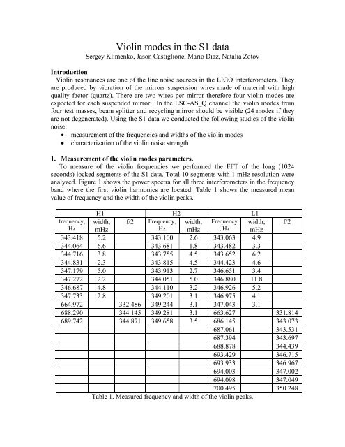
To measure of the violin frequencies we performed the FFT of the long (1024
seconds) locked segments of the S1 data. Total 10 segments with 1 mHz resolution were
analyzed. Figure 1 shows the power spectra for all three interferometers in the frequency
band where the first violin harmonics are located. Table 1 shows the measured mean
value of frequency and the width of the violin peaks.
H1 H2 L1
frequency, width, f/2 Frequency, width, Frequency width, f/2
Hz mHz
Hz mHz , Hz mHz
343.418 5.2 343.100 2.6 343.063 4.9
344.064 6.6 343.681 1.8 343.482 3.3
344.716 3.8 343.755 4.5 343.652 6.2
344.831 2.3 343.815 4.5 344.423 4.6
347.179 5.0 343.913 2.7 346.651 3.4
347.272 2.2 344.051 5.0 346.880 11.8
346.687 4.8 344.110 3.2 346.926 5.2
347.733 2.8 349.201 3.1 346.975 4.1
664.972 332.486 349.244 3.1 347.043 3.1
688.290 344.145 349.281 3.1 663.627 331.814
689.742 344.871 349.658 3.5 686.145 343.073
687.061 343.531
687.394 343.697
688.878 344.439
693.429 346.715
693.933 346.967
694.003 347.002
694.098 347.049
700.495 350.248
Table 1. Measured frequency and width of the violin peaks.

H1
H2
L1
Figure 1. Violin resonances in the S1 data.

The typical width of the violin resonances is 3-5 mHz (see Figure 2).
Figure 2. Width of the H2 violin modes.
We also measured the frequencies of some second harmonics. If we divide the frequency
of the second harmonics by two, the resulted frequency doesn’t match precisely any of
the first harmonics. Typically they are 10-50 mHz higher. One possible explanation is the
frequency shift due to the oscillation dumping
ω
2 2
= ω 0
− λ ,
where ω 0 is the violin angular frequency and λ is the dumping coefficient (1/λ is the
decay time). The difference between the second harmonic frequency divided by 2 and the
first harmonic frequency is approximately
3 2
∆ ω ≈ ω0λ
,
8
which could be 5-20 mHz for the decay time 185-60 sec respectively. In principle by
measuring the frequencies of two first harmonics one can measure the dumping
coefficient of the suspension wires, it’s hard to estimate the systematic errors of this
measurement.
2. Comparison with the previous measurements.
During the E7 and S1 runs we measured the frequencies and decay time of the L1
violin lines listed in Table 2.
E7
S1
frequency, Hz decay time, sec frequency, Hz decay time, sec
343.056 58 343.063 65
343.665 185, 140 343.652 48
346.932 64 346.926 61
Table 2. Comparison of frequencies and decay time for violin resonances measured
during E7 and S1 runs.

There is the order of 10 mHz difference between the S1 and E7 measurements, and we
believe these are the same lines. In both cases the measurement accuracy was ~1 mHz.
From here we may conclude that the violin frequency varies with time, which could be
due to the temperature variation. Of course it could be due to some unaccounted
systematic errors in the frequency measurement as well.
Table 2 shows also the comparison of the decay time measured for three violin lines for
E7 and S1 data. During the E7 run we measured the decay time directly by tracking the
amplitude of the resonances as a function of time (see Figure 2). For the S1 run the decay
time was estimated from the line width.
Figure 2. The decay of the 343.665 Hz line with decay time of 185 sec.
There is a reasonable agreement between the decay time of two lines at the frequencies
343.065 Hz and 346.932 Hz. However there is a considerable disagreement for the
343.665 Hz line. One possible explanation is that the 343.665 Hz line in fact consists of
two (or more) modes. Figure 3 shows the frequency distribution measured with the
LineMonitor during E7 run. There are three lines, which may correspond to different
modes. The lines at the 343.665 Hz and the 343.668 Hz have systematically different
decay time 140 sec and 185 sec respectively. Figure 3 shows the amplitude variation as a
function of time for the 343.668 Hz line.
Figure 3. Frequency distribution measured by the LineMonitor for 343.665 Hz line
during E7 run.

3. Tracking of the violin modes.
In the S1 data the amplitude of the violin resonances was very unstable. It was measured
by the LineMonitor, which has the integration time of one minute. Sometimes the violin
modes were excited in the beginning of the lock sections and usually they were barely
seen by the LineMonitor when the detectors were in lock. Table 3 shows the frequency
and duty cycle of the violin resonsnces, which can be seen by the LineMonitor.
f,
Hz f/2
duty,
% SNR
f,
Hz f/2
duty,
% SNR
f,
Hz f/2
duty,
% SNR
343.49 20.27 81.1 343.36 2.03 63.7 343.94 5.65 95.9
344.43 23.3 22.3 343.94 35.59 79.2 349.31 16.64 29.6
346.91 55.38 23.9 344.85 0.58 24.6 683.96 341.98 0.12 36.5
686.12 343.06 1.95 86.7 683.95 341.98 0.15 28.2 688.21 344.11 0.13 27.1
687.22 343.61 7.86 348.0 686.93 343.47 5.76 494.0
688.91 344.46 2.79 92.4 688.18 344.09 12.71 386.0
689.67 344.84 0.53 68.9
Table 3. Violin modes measured by the LineMonitor for the L1, H1, H2 interferometers.
The duty cycle was calculated as a fraction of the lock time when the violin amplitude
exceeds the LineMonitor threshold. Also the table shows the average signal to noise ratio
(SNR) for the data stretches when the modes are visible.
The average ratio of the violin signal PSD and the noise PSD (SNR), estimated from
the FFT analysis, is approximately 3.5 for the LineMonitor integration time. Therefore an
accurate tracking of the violin modes for S1 data with integration time of 1 minute is not
possible.
4. Other questions related to the violin noise investigation
• Does the violin noise present any threat for the ongoing data analysis?
Violin modes give small contribution into the variance of the detector output
signal. It’s not likely that the violin modes are correlated between different
interferometers, because violin frequencies are unique and the amplitudes are
non-stationary. Therefore they should not be a problem for the stochastic
searches. Besides they are located in the frequency band, which give small
contribution to the cross-correlation. The violin noise doesn’t seem to be a
problem for inspiral (too different signature) or continues waves searches. The
burst analysis may suffer from the violin noise, however at the moment there is no
evidence that it’s a dominant noise.
• Does the violin noise affect the detector operation?
• Do we need to track them during data taking? If yes, then how?
Perhaps we need to track large bursts of the violin noise associated with the
external excitation. Then the LineMonitor is an adequate tool for the violin
tracking.
• Is it important to know which mode is produced by which mirror?