Fluid mechanics, Bernoulli's principle and equation of continuity

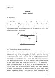
EXERCISE 5
Fluid mechanics, Bernoulli’s principle
and equation of continuity
6.1. Introduction
To begin with, let us define a fluid as “a substance as a liquid, gas or powder, that is
capable of flowing and that changes its shape at steady rate when acted upon by a force”. We
can distinguish four main types of fluid flow. The flow in which in each point occupied by
fluid its velocity doesn’t change in time is called stationary flow. Opposite, if velocity
vectors components of fluid elements are not the functions of the time, the flow is called nonstationary.
If the flow is smooth, such that neighbouring layers of the fluid slide by each other
smoothly, the flow is said to be streamline or laminar flow (Fig. 1a).. In this kind of flow,
each “particle” of the fluid follows a smooth path, called a streamline, and these paths do not
cross over one another. Above a certain speed, the flow becomes turbulent. Turbulent flow is
characterized by erratic, small whirlpool-like circles called eddy currents or eddies (Fig. 1b).
The transition from laminar to turbulent flow occurs when the energy (so also the velocity) of
the fluid “particles” becomes so high, that inner friction of the system (viscosity) can’t no
longer damp the eddies. At this moment we should notice that every turbulent flow is always
non-stationary, but laminar flow could be also stationary or non-stationary.
The character of flow is described by dimensionless Reynolds number. A few tiny drops of
ink or food colouring dropped into a moving liquid can quickly reveal whether the flow is
streamline or turbulent.
The fluid can be compressive or non-compressive. Liquids can be thinking of as noncompressive
fluids. Gases can be easily compressed, but the gases flows, if only the gas don’t
change its density during the flow, can be thinking of as non-compressive.
We will assume in this chapter that the fluid is essentially incompressible (no significant
variations in density) and that the flow is steady (so, no chance for turbulence).
22
36

FLUID MECHANICS. BERNOULLI’S PRINCIPLE AND EQUATION OF CONTINUITY
Fig. 1 (a) Streamline or laminar flow; (b) turbulent flow.
Let us consider the steady (laminar) flow of fluid through an enclosed tube or pipe as shown
in Fig. 6.2.
Fig. 6.2. Fluid flow through a pipe of varying diameter.
In such a pipe, the mass must be conserved, e.g. if we put mass m 1 into the pipe, then the same
mass m 2 =m 1 must flow out of this pipe (provided, the fluid is incompressible, since otherwise
the pipe can accumulate some mass, with no outgoing flow).
Consider infinitely small portion of mass, dm, put in a time dt into the pipe. From mass
conservation, we write”
dm
1
= dm 2
(6.1)
Knowing the relation of mass to volume and density, this reveals:
37

FLUID MECHANICS. BERNOULLI’S PRINCIPLE AND EQUATION OF CONTINUITY
dV
1ρ = dV2ρ
(6.2)
Volume, that falls into the pipe in a time dt is equal V=Adx, where A is the area of crosssection
of the pipe, and dx is the thickness of the mass layer, pumped in time dt. Substituting
this to above equation, keeping in mind the definition of velocity, we have
A dx
1
A v
1
1
1
= A
= A
2
2
v
dx
2
2
/ dt
(6.3)
This is the continuity equation for a fluid.
Equation (6.3) tells us that where the cross-sectional area is large the velocity is small, and
where the area is small the velocity is large. That this is reasonable and can be observed by
looking at a river. A river flows slowly through a meadow where it is broad, but speeds up to
torrential speed when passing through a narrow gorge. Have you ever wondered why smoke
goes up a chimney, why a car’s convertible top bulges upward at high speeds or how a
sailboat can move against the wind? There are examples of a principle worked out by Daniel
Bernoulli (1700-1782) in the early eighteenth century. In essence, Bernoulli’s principle states
that where the velocity of a fluid is high, the pressure is low.
Fig. 6.3 Fluid flow: for derivation of Bernoulli’s equation.
38

FLUID MECHANICS. BERNOULLI’S PRINCIPLE AND EQUATION OF CONTINUITY
Bernoulli developed an equation that expresses this principle quantitatively. To derive
Bernoulli’s equation, we assume the flow is steady and laminar the fluid is incompressible,
and the viscosity is small enough to be ignored. To be general, we assume the fluid is flowing
in a tube of nonuniform cross section that varies in height above some reference level, Fig 6.3.
Bernoulli’s equation in such system is simply an expression of the work-energy theorem.
What is the energy of the fluid at some position in the pipe? It is a sum of kinetic energy,
potential gravitational energy, and internal energy, put by external force. For a mass element
dm=ρAdx, we can write this as
E = E + E + E
(6.4.)
K
P
i
2
dmv
E
K
= (6.5.)
2
E P
= dmgh
(6.6.)
E i
= pdV
(6.7.)
The energy components have self-explanatory meaning, kinetic energy is defined as usual,
gravitational potential energy also. A comment needs only be done on the internal energy. To
put the mass element dm into the pipe, we have to overcome some pressure p, which exists in
that pipe. This pressure generates a force F = pA that resists the motion. Moving by dx, a
work needs to be done on the fluid,
W = Fdx = pAdx = pdV . This work changes to the
internal energy of the fluid.
We can divide the energy equation (6.4) by dV to obtain the Bernoulli equation, which states,
that the energy of a fluid doesn’t change in the flow. This is reasonable, since no energy is put
to the fluid anywhere else, than in its input. Thus we have, keeping in mind that dm=ρdV, that
1 2
P + ρv
+ ρgy
= constant
(6.8)
2
39

FLUID MECHANICS. BERNOULLI’S PRINCIPLE AND EQUATION OF CONTINUITY
or equivalently, taking two points in the pipe and evaluating above equation for both of them,
1 2
1 2
P1 + ρv1
+ ρgy1
= P2
+ ρv
2
+ ρgy
2
(6.9)
2
2
This is Bernoulli’s equation. [if there is no flow (v 1 =v 2 =0), then eq. (6.9) reduces to the
hydrostatic equation: P 2 -P 1 =-ρg(y 2 -y 1 ).]
6.2. Measurements
Experimental setup is shown on the figure below:
Fig. 6.4. Experimental setup.
The experimental setup consists of pomp, which pumps the water from container A, through
glass pipe with two different cross-section areas to container B. In order to avoid high
40

FLUID MECHANICS. BERNOULLI’S PRINCIPLE AND EQUATION OF CONTINUITY
pressure increase in the system when the pump is turn on with valve nr.1 closed, a part of
water goes back to container A. There are two valves in the system: earlier mentioned one
(nr.1), which allows us to control water flow rate in the system (it should always be closed
when you turn on the pump) and valve nr.2 (it should be always open).
In two part of the glass pipe – in wide and in narrow – pressure, manometric tubes are used to
measure the static pressure in the system. Such kind of measurements doesn’t disturb the
water flow in the glass pipe. Bernoulli’s law says that the pressure will be different in these
two points of glass pipe. If two manometric tubes will be connected as it is shown on the
fig.6.4, we obtain manometric tube and the observed difference of the liquid level, will be
equal to the difference of static pressure between two points in the pipe. The knowledge of
pressure difference p 1 –p 2 isn’t enough to determine the rate flow of the water. We need to
assume the flow continuity and we need to know the cross-section areas A 1 and A 2
To begin with you have to measure the diameter of two cross sections (1 and 2, see the Fig.
6.4) of the pipe and calculate the cross-sections areas A 1 and A 2. .
Next you should prepare the system to perform the experiment.
Attention!!!
Before you turn on the pump, be sure that the valve nr.2 is open (the arm should be parallel in
respect to the hose) and valve nr.1 is closed (the arm should be perpendicular in respect to the
hose). Be also sure that the container A is filled with water, the container B is empty and that
all connections are ok (see the scheme).
Never turn on the pump without checking valves configurations and hoses connections!!!!
The experiment:
• Before each measurement, note the initial difference of liquid level in manometric
tube. (it should be not greater than 15mm)
• After checking of valves configurations and connections turn on the pump.
41

FLUID MECHANICS. BERNOULLI’S PRINCIPLE AND EQUATION OF CONTINUITY
• The measurements should be de tree times, for tree different open degree of valve nr.1.
• After valve nr.1 opening, you should notice times needed to fill the container B with
the water volumes equal to 5L, 10L and 15L.
• In the same time, note the liquid level difference in the manometric tube ∆h for given
volume.
• After finishing of measurements, very slowly close the valve nr.1 and then turn off the
pump (exactly in the specified order).
• After finishing of given measurement, you should pour the water from container B to
container A and repeated the measurements for another valve nr.1 open degree.
Attention!!!
The container A should always be filled with water to marked minimum level. If the water
level in container A reaches its minimum, you should instantly turn off the pump.
Calculations:
From equation of continuity and Bernoulli’s equation we can express the velocity at cross
section 2 as:
v = (6.10)
1A1
v
2A
2
A
2
v
1
= v
2
(6.11)
A1
p
2
2
v1
v
2
+ ρ
w
= p
2
+
w
(6.12)
2
2
1
ρ
p
2 2
2
v
2A
2
v
2
+ ρ
w
= p
2 2
+
w
(6.13)
2A
2
1
ρ
1
2
− 2∆pA
v = (6.14)
ρ
2
w
1
2 2
( A − A )
1
2
42

FLUID MECHANICS. BERNOULLI’S PRINCIPLE AND EQUATION OF CONTINUITY
where ∆p is the pressure difference between cross-sections A2 i A1:
-∆p = -(p 2 -p 1 ) = p 1 -p 2
The pressure difference, which is equal to a liquid hydrostatic pressure, should be measure
using the difference in liquid level in manometric tube:
p
− p ρ hg
(6.15)
1 2
=
m
where:
ρ m – is the density of manometric liquid
h – is the height difference between two arms of manometer.
So, finally we can write
v
2
2
2ρ
hgA
= (6.16)
ρ
w
m 1
2 2
( A − A )
1
2
Another way of calculating v 2 is by means of measuring the volume of water flowing out of
tube over certain time t
2
πd
2
V = v
2
t
(6.17)
4
or
4V
= (6.18)
πd
t
v
2 2
2
The data should be collected in a table 6.1
In the given measurements (for given valve nr.1 open degree) for each measured pair (volume
of the water in container B – the time needed to reach such volume) the value of ∆h is
constant (such as measured at the end of given measurements).
Table 6.1
43

FLUID MECHANICS. BERNOULLI’S PRINCIPLE AND EQUATION OF CONTINUITY
No. d 1 A 1 d 2 A 2 h V t v 2a
from
eq. 6.16
v 2b
from
eq. 6.18
6.3. Results, calculations and uncertainty.
1. From the data collected in Table 6.1 calculate the average values of
1
v (6.19)
n
2a
= ∑ v
2a i
n i=
1
and
1
v (6.20)
n
2b
= ∑ v
2b i
n i=
1
Estimate the uncertainty of the measured values of velocities by using below formula for eqs.
6.16 and 6.18 respectively.
dv
2
2
2
2
2 ⎜
dh + dA1
+ dA2
∂h
⎟ ⎜
1
∂A
⎟ ⎜
1
∂A
⎟
2
2
2
=
⎛ ∂v
⎜
⎞
⎟
⎛ ∂v
⎜
⎞
⎟
⎛ ∂v
⎜
⎞
⎟
(6.21)
⎝ ⎠ ⎝ ⎠ ⎝ ⎠
Assume: ρ m , ρ w = 1000kg/m 3
The final result reads
v = ±
(6.22)
2
v
2
dv
2
44

FLUID MECHANICS. BERNOULLI’S PRINCIPLE AND EQUATION OF CONTINUITY
2. Having v 2 , calculate v 1
a) from the continuity equation A 1 v 1 = A 2 v 2
2 2
b) from the Bernoulli equation ρ (v − v ) = p
1 2
∆
Plot these values in and v 1 -v 2 chart, and compare the tangent of revealed slope with the
measured value of
A
1 .
A
2
6.4. Questions
1. Derive the equation of continuity.
2. The equation of continuity is a special case of some conservation principle. Describe
this principle.
3. Derive the Bernoulli’s equation.
4. The Bernoulli’s equation is a special case of some conservation principle. Describe
this principle.
5. What kind of assumptions you have to make to derive these equations?
6. Explain how a water aspirator works.
7. Explain principle of lifting force in airplane.
8. Explain the experiment with the coin that was presented during the lecture.
9. What is “The Reynolds number”?
10. During measurements performance, rise of flowing water in the glass tube can be
observed. Describe this phenomena.
6.5 References
1. Szczeniowski S., Fizyka Doświadczalna, Część I, Mechanika i Akustyka, PWN,
Warszawa, 1980
2. Resnick R., Halliday D., Fizyka, Tom I, PWN, Warszawa, 1966
3. Giancoli D.C., Physics. Principles with Applications, Prentice Hall, 2000
4. Young H.D., Freedman R.A., University Physics with Modern Physics, Addison-Wesley
Publishing Company, 2000
5. Szydłowski H., Pracownia fizyczna, PWN, Warszawa, 1994
45