7. The Smith Chart

W.C.Chew
ECE 350 Lecture Notes
7. The Smith Chart
We have seen from Equation (6.9) that a generalized impedance can be
dened as
V
Z(z) = ~ (z)
~I(z) = Z e ;jz + v e +jz
0
e ;jz ; v e
+jz:
(1)
The above can be written as
1+ v e 2jz
Z(z) =Z 0
1 ; v e = Z 1+;(z)
2jz 0
1 ; ;(z) (2)
where ;(z) is as dened in (6.16). When z = 0, Z(0) = Z L , and ;(0) = v ,
and (2) becomes (6.25). Hence (6.25) is a special case of (2). We can introduce
a normalized generalized impedance to be
Similarly,
Z n (z) = Z(z)
Z 0
= 1+;(z)
1 ; ;(z) : (3)
;(z) = Z n(z) ; 1
Z n (z)+1 : (4)
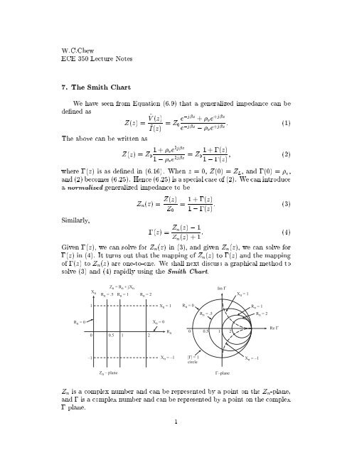
Given ;(z), we can solve for Z n (z) in (3), and given Z n (z), we can solve for
;(z) in (4). It turns out that the mapping of Z n (z) to;(z) and the mapping
of ;(z) toZ n (z) are one-to-one. We shall next discuss a graphical method to
solve (3) and (4) rapidly using the Smith Chart.
X n
Z n = R n + jX n
R n = .5 R n = 1 R n = 2
Im Γ
X n = 1
1
X n = 1
R n = 0
R n = 1
R n = .5
R n = 2
R n = 0
0 0.5 1 2
X n = 0
R n
0 0.5 1 2
Re Γ
–1
X n = –1
|Γ| = 1
circle
X n = –1
Z n – plane
Γ–plane
Z n is a complex number and can be represented by a point on the Z n -plane,
and ; is a complex number and can be represented by apoint on the complex
; plane.
1

We noted that from Equation (4) that:
(i) When Z n =0 ;=;1.
(ii) When Z n =1,or R n =1X n =0 ;=0.
(iii) When Z n !1in any direction, ; ! 1.
(iv) When Z n = jX n j;j =1.
(v) When Z n = j, or R n =0X n =1 ;=j.
(vi) When Z n = ;j, or R n =0X n = ;1 ;=;j.
If one works out the mapping from Z n -plane to ;-plane completely, one
nds that the R n = 0 line on Z n -plane maps onto the unit-circle on the ;-
plane. Furthermore, the other R n = constant lines map into circles as shown.
The X n = constant lines map into arcs like the X n 1 lines as shown. Hence,
if one puts grids on the ;-plane, one can read o the R n and X n associated
with the corresponding ; immediately, and, given the value of ;, one can
read o the values of R n and X n immediately.
The mappings (3) and (4) are known as bilinear transforms. A bilinear
transform always maps a circle onto a circle.
Properties of a Smith Chart
(i) The normalized admittance Y n = 1=Z n , or the reciprocal of Z n , can be
found easily from a Smith Chart, because
Zn
;= Z n ; 1
Z n +1 = 1 ; 1
1+ 1
Zn
= 1 ; Y n
1+Y n
= ; Y n ; 1
Y n +1 : (5)
(ii) The change of impedance along the line is obtained by adding or subtracting
phase to ;(z) via the relationship
;(z) = v e 2jz : (6)
(iii)
VSWR = 1+j vj
1; j v j = R nmax (7)
since the Smith Chart is a graphical tool to solve Equation (7), and j v j
is real, corresponding to a number on the X n = 0 line. Notice that
1 < VSWR < 1 always.
2