Real-time Image-Based Motion Detection Using Color and Structure
Real-time Image-Based Motion Detection Using Color and Structure
Real-time Image-Based Motion Detection Using Color and Structure

Create successful ePaper yourself
Turn your PDF publications into a flip-book with our unique Google optimized e-Paper software.
<strong>Real</strong>-<strong>time</strong> <strong>Image</strong>-<strong>Based</strong> <strong>Motion</strong> <strong>Detection</strong> <strong>Using</strong><br />
<strong>Color</strong> <strong>and</strong> <strong>Structure</strong><br />
Manali Chakraborty <strong>and</strong> Olac Fuentes<br />
Dept. of Computer Science,<br />
University of Texas at El Paso<br />
500 West University Avenue,<br />
El Paso, TX -79902.<br />
mchakraborty@miners.utep.edu, ofuentes@utep.edu<br />
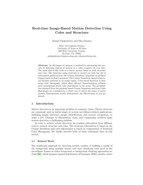
Abstract. In this paper we propose a method for automating the process<br />
of detecting regions of motion in a video sequence in real <strong>time</strong>.<br />
The main idea of this work is to detect motion based on both structure<br />
<strong>and</strong> color. The detection using structure is carried out with the aid of<br />
information gathered from the Census Transform computed on gradient<br />
images based on Sobel operators. The Census Transform characterizes local<br />
intensity patterns in an image region. <strong>Color</strong>-based detection is done<br />
using color histograms, which allow efficient characterization without<br />
prior assumptions about color distribution in the scene. The probabilities<br />
obtained from the gradient-based Census Transform <strong>and</strong> from <strong>Color</strong><br />
Histograms are combined in a robust way to detect the zones of active<br />
motion. Experimental results demonstrate the effectiveness of our approach.<br />
1 Introduction<br />
<strong>Motion</strong> detection is an important problem in computer vision. <strong>Motion</strong> detectors<br />
are commonly used as initial stages in several surveillance-related applications,<br />
including people detection, people identification, <strong>and</strong> activity recognition, to<br />
name a few. Changes in illumination, noise, <strong>and</strong> compression artifacts make<br />
motion detection a challenging problem.<br />
In order to achieve robust detection, we combine information from different<br />
sources, namely structure <strong>and</strong> color. The structure information is based on the<br />
Census Transform <strong>and</strong> color information is based on computation of Temporal<br />
<strong>Color</strong> Histograms. We briefly describe both of these techniques later in this<br />
section.<br />
1.1 Related Work<br />
The traditional approach for detecting motion consists of building a model of<br />
the background using multiple frames <strong>and</strong> then classifying each pixel in the<br />
surveillance frames as either foreground or background. Existing approaches include<br />
[10], which proposes spatial distribution of Gaussian (SDG) models, where
motion compensation is only approximately extracted, [11], which models each<br />
pixel as a mixture of Gaussians <strong>and</strong> uses an online approximation to update the<br />
model <strong>and</strong> [8], which proposes an online method based on dynamic scene modeling.<br />
Recently, some hybrid change detectors have been developed that combine<br />
temporal difference imaging <strong>and</strong> adaptive background estimation to detect regions<br />
of change [4]. Huwer et al. [4] proposed a method of combining a temporal<br />
difference method with an adaptive background model subtraction scheme to<br />
deal with lighting changes. Even though these approaches offer somewhat satisfactory<br />
results, much research is still needed to solve the motion detection<br />
problem, thus complementary <strong>and</strong> alternate approaches are worth investigating.<br />
In this paper we propose an approach to motion detection that combines information<br />
extracted from color with information extracted from structure, which<br />
allows a more accurate classification of foreground <strong>and</strong> background pixels. We<br />
model each pixel using a combination of color histograms <strong>and</strong> histograms of local<br />
patterns derived from the Modified Census Transform [1], applied to gradient<br />
images.<br />
1.2 The Census Transform<br />
The Census Transform is a non-parametric summary of local spatial structure.<br />
It was originally proposed in [16] in the context of stereo-matching <strong>and</strong> later<br />
extended <strong>and</strong> applied to face detection in [1]. It has also been used for optical<br />
flow estimation [12], motion segmentation [14], <strong>and</strong> h<strong>and</strong> posture classification<br />
<strong>and</strong> recognition under varying illumination conditions [6].<br />
The main features of this transform are also known as structure kernels <strong>and</strong><br />
are used to detect whether a pixel falls under an edge or not. The structure<br />
kernels used in this paper are of size 3 × 3, however, kernels can be of any<br />
size m × n . The kernel values are usually stored in binary string format <strong>and</strong><br />
later converted to decimal values that denote the actual value of the Census<br />
Transform.<br />
In order to formalize the above concept, let us define a local spatial neighborhood<br />
of the pixel x as N(x), with x /∈ N(x). The Census Transform then generates<br />
a bit string representing which pixels in N(x) have an intensity lower than<br />
I(x). The formal definition of the process is as follows: Let a comparison function<br />
ζ(I(x), I(x ′ )) be 1 if I(x) < I(x ′ ) <strong>and</strong> 0 otherwise, let ⊗ denote the concatenation<br />
operation, then the census transform at x is defined as C(x) = ⊗ ζ(I(x), I(y)).<br />
This process is shown graphically in Figure 1.<br />
1.3 The Modified Census Transform<br />
The Modified Census Transform was introduced as a way to increase the information<br />
extracted from a pixel’s neighborhood [1]. In the Modified Census<br />
Transform , instead of determining bit values from the comparison of neighboring<br />
pixels with the central one, the central pixel is considered as part of<br />
the neighborhood <strong>and</strong> each pixel is compared with the average intensity of the<br />
neighborhood. Here let N(x) be a local spatial neighborhood of pixel at x, so
Fig. 1. The intensity I ( 0) denotes the value of the central pixel, while the neighboring<br />
pixels have intensities I (1) ,I (2) ... I (8) . The value of the Census Transform<br />
is generated by a comparison function between the central pixel <strong>and</strong> its neighboring<br />
pixels.<br />
that N ′ (x) = N(x) ∪ {x}. The mean intensity of the neighboring pixels is denoted<br />
byI(¯x). So using this concept we can formally define the Modified Census<br />
Transform as follows where all 2 9 kernel values are defined for the 3×3 structure<br />
kernels considered.<br />
C(x) = ⊗ ζ(I(¯x), I(y))<br />
1.4 Gradient <strong>Image</strong><br />
The Gradient <strong>Image</strong> is computed from the change in intensity in the image.<br />
We used the Sobel operators, which are defined below. The gradient along the<br />
vertical direction is given by the matrix G y <strong>and</strong> the gradient along the horizontal<br />
direction is given by G x . From G x <strong>and</strong> G y we then generate the gradient<br />
magnitude.<br />
⎛ ⎞<br />
⎛ ⎞<br />
+1 +2 +1<br />
+1 0 −1<br />
G y = ⎝ 0 0 0 ⎠ G x = ⎝+2 0 −2⎠<br />
−1 −2 −1<br />
+1 0 −1<br />
The gradient magnitude is then given by G =<br />
√<br />
G 2 x + G 2 y. Our proposed<br />
Census Transform is computed from this value of magnitude derived from the<br />
gradient images.<br />
1.5 Temporal <strong>Color</strong> Histogram<br />
The color histogram is a compact representation of color information corresponding<br />
to every pixel in the frame. They are flexible constructs that can be built<br />
from images in various color spaces, whether RGB, chromaticity or any other
color space of any dimension. A histogram of an image is produced first by discretisation<br />
of the colors in the image into a number of bins, <strong>and</strong> counting the<br />
number of image pixels in each bin. <strong>Color</strong> Histograms are used instead of any<br />
other sort of color cluster description [3,5,7,9], due to its simplicity, versatility<br />
<strong>and</strong> velocity, needed in tracking applications. Moreover, it has been vastly proven<br />
its use in color object recognition by color indexing [2,13]. However the major<br />
shortcoming of detection using color is that it does not respond to changes to<br />
illumination <strong>and</strong> object motion.<br />
2 Proposed Algorithm<br />
The proposed algorithm mainly consists of two parts; the training procedure <strong>and</strong><br />
the testing procedure. In the training procedure we construct a look up table<br />
using the background information. The background probabilities are computed<br />
based on both the Census Transform <strong>and</strong> <strong>Color</strong> Histograms. Here we consider a<br />
pixel in all background video frames <strong>and</strong> then identify its gray level value as well<br />
as the color intensities corresponding to the RGB color space which are then<br />
used to compute the probabilities. In the testing procedure the existing look up<br />
is used to retrieve the probabilities from it.<br />
2.1 Training<br />
Modified Census Transform The modified Census Transform generates structure<br />
kernels in the 3×3 neighborhood but the kernel values are based on slightly<br />
different conditions. To solve the problem of detecting regions of uniform color<br />
we use base 3 patterns instead of base 2 patterns. Now, let N(x) be a local spatial<br />
neighborhood of the pixel at x so that N ′ (x) = N(x) ∪ {x}. Then the value of<br />
the Modified Census Transform in this algorithm is generated representing those<br />
pixels in N(x) which have an intensity significantly lower, significantly greater or<br />
similar to the mean intensity of the neighboring pixels. This is denoted by I(¯x)<br />
<strong>and</strong> the comparison function is defined as:<br />
⎧<br />
⎨ 0 if I(x) < I(¯x) − λ<br />
ζ(I(x), I(¯x)) = 1 if I(x) > I(¯x) + λ<br />
⎩<br />
2 otherwise<br />
Where λ is a tolerance constant. Now if ⊗ denotes the concatenation operation,<br />
the expression for the Modified Census Transform in terms of the above<br />
conditions at x becomes;<br />
C(x) = ⊗ ζ(I(¯x), I(y))<br />
Once the value of the Census Transform kernel has been computed it is used<br />
to index the occurrence of that pixel in the look up. So for every one of the pixels<br />
we have kernel values which form the indices of the look up table. For a particular<br />
index in the look up the contents are the frequencies of pixel occurrences for that<br />
value of kernel in all of the frames. When the entire lookup has been constructed<br />
from the background video we compute the probabilities which are then used<br />
directly at the <strong>time</strong> of testing.
Fig. 2. The frequencies corresponding to the known kernel indices are stored in<br />
the given look up for one pixel. The frequency belonging to a particular kernel<br />
designates the no of frames for that pixel which has the same kernel value.<br />
<strong>Color</strong> Histograms The color probabilities are obtained in a similar fashion but<br />
using the concept of color histograms. In this case initially the color intensities<br />
are obtained in RGB format <strong>and</strong> based on these values the color cube/bin corresponding<br />
to the Red-Green-Blue values of the pixel is determined. Since each<br />
color is quantized to 4 levels the sum total of 4 3 = 64 such bins are possible. So<br />
every pixel has a corresponding counter containing 64 values <strong>and</strong> the color cube<br />
values form the indices of this counter look up. The color counter contains the<br />
frequency of that pixel having a particular color across all frames.<br />
Fig. 3. The color cube displays one of the total 4 3 = 64 bins possible.<br />
2.2 Testing<br />
The frames from the test video are used to obtain the pixel intensities in both<br />
gray level <strong>and</strong> R-G-B color space. Then for every one of these pixels we compute
again the Census Transform which serves as an index in the existing look up<br />
for the same pixel <strong>and</strong> the probability corresponding to that index is retrieved.<br />
In this way we use the probabilities corresponding to all pixels in any frame<br />
being processed in real <strong>time</strong>. Fig. 4 demonstrates the concept of testing where<br />
initially the Modified Census Transform is computed for pixel 0 based on its 3<br />
× 3 neighborhood. The kernel value is used as an index for the look up table<br />
already constructed to retrieve the required frequency. Here the value of the<br />
Census Transform is 25 which then serves as the index. The frequency 33 actually<br />
represents that for pixel 0 there are 33 frames which have the same value of kernel<br />
of 25.<br />
In the case of color the same scheme is used where every pixel is split into<br />
its R-G-B color intensities <strong>and</strong> then the color bin for it is computed. This is<br />
then used as the index to retrieve the value of the probability existing for that<br />
particular index from the color counter look up constructed before. So this gives<br />
us all corresponding probabilities of pixels belonging to any frame at any instant<br />
of <strong>time</strong>. Once we have the color <strong>and</strong> the Census Transform probabilities we<br />
combine the information from both the color <strong>and</strong> Census matrices to detect the<br />
region of interest.<br />
Fig. 4. The Modified Census Transform generates the value 25 which then serves<br />
as index for the already constructed look up table during training. The frequency<br />
33 gives the frequency of occurrence of frames for that pixel having the same<br />
value of kernel.<br />
3 Results<br />
The first set of experiments was conducted on a set of frames in an indoor<br />
environment with uniform lighting <strong>and</strong> <strong>and</strong> applying the Census Transform to<br />
intensity images. This detection of this set of experiments is shown in Figure<br />
5 <strong>and</strong> Figure 6. The second set includes frames from videos also taken in an
indoor environment, now we used gradient information to compute the Census<br />
Transform. The results from this set are displayed in Figure 7. Finally the outdoor<br />
training is carried out with a set of frames where there is variation in light<br />
intensity as well as fluctuations in wind velocity observed from Figure 8.<br />
Fig. 5. Results from detection using Census Transform probabilities without<br />
using gradient information<br />
Fig. 6. Results from detection using color probabilities<br />
4 Conclusion <strong>and</strong> Future Work<br />
We have presented a method for motion detection that uses color <strong>and</strong> structure<br />
information. Our method relies on two extension to the Census transform to<br />
achieve robust detection, namely, the use of gradient information <strong>and</strong> a basethree<br />
encoding. <strong>Using</strong> gradient information allows to more accurately detect the<br />
outlines of moving objects, while our base-three encoding allows to deal effectively<br />
with regions of relatively uniform color. The efficiency of the approach
Fig. 7. Results from detection using gradient information to compute Census<br />
Transform<br />
is demonstrated by the fact that the entire procedure can be easily carried out<br />
in real <strong>time</strong>. Current work include developing a dynamic update of the background<br />
model, developing methods for taking advantage of gradient direction<br />
information, <strong>and</strong> exploring other color spaces.<br />
References<br />
1. Bernhard Froba <strong>and</strong> Andreas Ernst. Face detection with the modified census<br />
transform. In Sixth IEEE International Conference on Automatic Face <strong>and</strong> Gesture<br />
Recognition, pages 91– 96, Erlangen, Germany, May 2004.<br />
2. Brian V. Funt <strong>and</strong> Graham D. Finlayson. <strong>Color</strong> constant color indexing. IEEE<br />
Transaction on Pattern Analysis <strong>and</strong> Machine Intelligence, 17(5):522–529, 1995.<br />
3. B. Heisele, U. Kressel, <strong>and</strong> W. Ritter. Tracking non-rigid, moving objects based<br />
on color cluster flow. In Proceedings of 1997 IEEE Computer Society Conference<br />
on Computer Vision <strong>and</strong> Pattern Recognition, pages 257–260, San Juan, Puerto<br />
Rico, June 1997.<br />
4. Stefan Huwer <strong>and</strong> Heinrich Niemann. Adaptive change detection for real-<strong>time</strong><br />
surveillance applications. In Third IEEE International Workshop on Visual<br />
Surveillance, pages 37–46, Dublin, Irel<strong>and</strong>, 2000.<br />
5. Daesik Jang <strong>and</strong> Hyung-Il Choi. Moving object tracking using active models. Proceedings<br />
of 1998 International Conference on <strong>Image</strong> Processing (ICIP 98), 3:648–<br />
652, Oct 1998.<br />
6. Agnes Just, Yann Rodriguez, <strong>and</strong> Marcel Sebastien. H<strong>and</strong> posture classification<br />
<strong>and</strong> recognition using the modified census transform. In Proceedings of the 7th
Fig. 8. Results from detection using Census Transform based on gradient images<br />
in outdoor environment<br />
International Conference on Automatic Face <strong>and</strong> Gesture Recognition (FGR06),<br />
pages 351–356, 2006.<br />
7. S. J. McKenna, Y. Raja, <strong>and</strong> S. G. Gong. Tracking colour objects using adaptive<br />
mixture models. <strong>Image</strong> <strong>and</strong> Vision Computing, 17(3/4):225–231, March 1999.<br />
8. Antoine Monnet, Anurag Mittal, Nikos Paragios, <strong>and</strong> Visvanathan Ramesh. Background<br />
modeling <strong>and</strong> subtraction of dynamic scenes. In ICCV ’03: Proceedings of<br />
the Ninth IEEE International Conference on Computer Vision, pages 1305–1312,<br />
Washington, DC, USA, 2003.<br />
9. T. Nakamura <strong>and</strong> T. Ogasawara. Online visual learning method for color image<br />
segmentation <strong>and</strong> object tracking. Proceedings of 1999 IEEE/RSJ International<br />
Conference on Intelligent Robots <strong>and</strong> Systems (IROS ’99), 1:222–228 vol.1, 1999.<br />
10. Ying Ren <strong>and</strong> Ching-Seng Chua. <strong>Motion</strong> detection with non-stationary background.<br />
In Proceedings of the 11th International Conference on <strong>Image</strong> Analysis<br />
<strong>and</strong> Processing, Palermo, Italy, September 2001.<br />
11. Chris Stauffer <strong>and</strong> W.E.L Grimson. Adaptive background mixture models for<br />
real <strong>time</strong> tracking. IEEE Computer Society Conference on Computer Vision <strong>and</strong><br />
Pattern Recognition, 2:252, 1999.<br />
12. Fridtjof Stein. Efficient computation of optical flow using the census transform.<br />
In 26th Symposium of the German Association for Pattern Recognition (DAGM<br />
2004), pages 79–86, Tubingen, August 2004.<br />
13. M. J. Swain <strong>and</strong> D. H. Ballard. <strong>Color</strong> indexing. International Journal of Computer<br />
Vision, 7(1):11–32, November 1991.<br />
14. Kunio Yamada, Kenji Mochizuki, Kiyoharu Aizawa, <strong>and</strong> Takahiro Saito. <strong>Motion</strong><br />
segmentation with census transform. Advances in Mul<strong>time</strong>dia Information Processing<br />
- PCM 2001, 2195:903–908, January 2001.<br />
15. N. Yamamoto <strong>and</strong> K. Matsumoto. Obstruction detector by environmental adaptive<br />
background image updating. ERTICO, editor,4th World Congress on Intelligent<br />
Transport Systems, 4:1–7, October 1997.<br />
16. Ramin Zabih <strong>and</strong> John Woodfill. Non-parametric local transforms for computing<br />
visual correspondence. In European Conference on Computer Vision, pages 151–<br />
158, Stockholm, Sweden, May 1994.