Langevin thermostat for rigid body dynamics - Lammps

234101-10 Davidchack, Handel, and Tretyakov J. Chem. Phys. 130, 234101 2009
Γ, ps −1
10 3 γ,ps −1
10 2
10 1
8
7
6
τU, ps
5
4
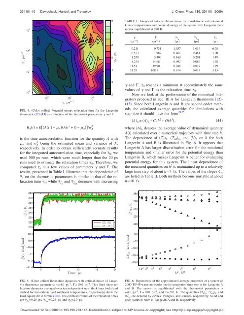
TABLE I. Integrated autocorrelation times for translational and rotational
kinetic temperatures and potential energy of the system with Langevin thermostat
equilibrated at 270 K.
ps −1
ps −1
¯Ttr
ps
¯Trot
ps
¯U
ps
0.211 0.731 1.037 1.019 6.08
0.573 1.987 0.461 0.481 3.00
1.558 5.400 0.169 0.201 1.48
4.234 14.68 0.092 0.086 1.78
11.51 39.90 0.048 0.039 1.99
31.29 108.5 0.014 0.017 3.15
10 0
10 0 10 1 10 2
FIG. 4. Color online Potential energy relaxation time for the Langevin
thermostat 12-13 as a function of the thermostat parameters and .
R A t = EAt − A At + t − A / A
2
is the time autocorrelation function for the quantity A with
A and A 2 being the estimated mean and variance of A,
respectively. In order to obtain sufficiently accurate results
for the integrated autocorrelation time, especially for ¯U, we
used 500 ps runs, which were much longer than the 20 ps
runs used to estimate the relaxation times A . Therefore, we
computed ¯A at a few values of parameters and . The
results, presented in Table I, illustrate that the dependence of
¯A on the thermostat parameters is similar to that of the relaxation
time A : while ¯Ttr and ¯Trot decrease with increasing
3
2
and , ¯U reaches a minimum at approximately the same
values of and as the relaxation time U .
Now we look at the performance of the numerical integrators
proposed in Sec. III A for Langevin thermostat 12-
13. Since both Langevin A and B are second-order methods,
the calculated average quantities for simulations with
step size h should have the form 20,25
A h = A 0 + C A h 2 + Oh 3 ,
44
where A h denotes the average value of dynamical quantity
At calculated over a numerical trajectory with time step h.
The dependence of T tr h , T rot h , and U h on h for both
Langevin A and B is illustrated in Fig. 6. It appears that
Langevin A has larger discretization error for the rotational
temperature and smaller error for the potential energy than
Langevin B, which makes Langevin A better for evaluating
potential energy for this system. The linear dependence of
the measured quantities on h 2 is maintained up to a relatively
large time step of about h=7 fs. The values of the slopes C A
are listed in Table II. Both methods become unstable at about
h=10 fs.
T , K
U, kcal/mol
280
270
260
250
240
230
220
210
−10.4
−10.6
−10.8
−11
−11.2
−11.4
T tr (t)
T rot (t)
0 5 10 15 20
Time, ps
〈T 〉h, K
〈U〉h, kcal/mol
280
260
240
220
200
−9.8
−10
−10.2
−10.4
−10.6
12 2 3 2 4 2 5 2 6 2 7 2 8 2 9 2
h 2 , fs 2
FIG. 5. Color online Relaxation dynamics with optimal choice of Langevin
thermostat parameters: =4.0 ps −1 , =10.0 ps −1 . Thin lines show relaxation
dynamics averaged over ten independent runs, thick lines solid and
dashed for translational and rotational temperatures, respectively show the
least-squares fit to formula 40. The estimated values of the relaxation times
are Ttr =0.28 ps, Trot =0.26 ps, and U =2.0 ps.
FIG. 6. Dependence of the approximated average properties of a system of
2000 TIP4P water molecules on the integration time step h for Langevin A
and B. The system is equilibrated with the thermostat parameters
=4.0 ps −1 , =10.0 ps −1 , and T=270 K. The quantities T tr h , T rot h , and
U h are denoted by circles, triangles, and squares, respectively. Solid and
open symbols refer to Langevin A and B, respectively.
Downloaded 12 Sep 2009 to 193.190.253.147. Redistribution subject to AIP license or copyright; see http://jcp.aip.org/jcp/copyright.jsp