Langevin thermostat for rigid body dynamics - Lammps

More documents

Recommendations

Info

234101-12 Davidchack, Handel, and Tretyakov J. Chem. Phys. 130, 234101 2009 0.3 280 270 10 3 ν, fs 0.25 0.2 Trot, K 260 250 240 230 Γ, ps −1 10 2 0.15 τTrot ,ps 220 210 −10.4 10 1 10 0 10 2 10 3 0.05 FIG. 10. Color online Rotational temperature relaxation time for the gradient-Langevin thermostat 14-15 as a function of the thermostat parameters and . what surprising finding of this experiment is that even for small values of the relaxation time is much smaller here than in the case of Langevin thermostat see Fig. 3. 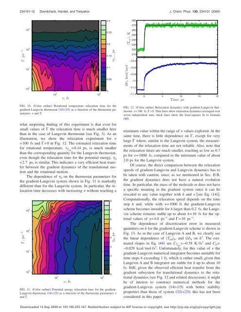Asan illustration, we show the relaxation experiment for =100 fs and =0 in Fig. 12. The estimated relaxation time for rotational temperature, Trot =0.14 ps, is much smaller than the corresponding quantity for the Langevin thermostat, even though the relaxation time for the potential energy, U =2.7 ps, is similar. This indicates a very efficient heat transfer between the gradient dynamics of the translational motion and the rotational motion. The dependence of U on the thermostat parameters for the gradient-Langevin system shown in Fig. 11 is markedly different than for the Langevin system. In particular, the relaxation time decreases with increasing without reaching a Γ, ps −1 10 3 10 2 10 1 10 0 ν,fs 10 2 10 3 0.1 0 8 7 6 5 τU, ps FIG. 11. Color online Potential energy relaxation time for the gradient- Langevin thermostat 14-15 as a function of the thermostat parameters and . 4 3 2 1 0 U, kcal/mol −10.6 −10.8 −11 −11.2 −11.4 0 5 10 15 20 Time, ps FIG. 12. Color online Relaxation dynamics with gradient-Langevin thermostat: =100 fs, =0. Thin lines show relaxation dynamics averaged over seven independent runs, thick lines show the least-squares fit to formula 40. minimum value within the range of values explored. At the same time, there is little dependence on , except for very large where, similar to the Langevin system, the measurements of the relaxation time are not reliable. Also, note that the relaxation times are much smaller, reaching as low as 0.7 ps for =1000 fs, compared to the minimum value of about 2.0 ps for the Langevin system. Of course, the direct comparison between the relaxation speeds of gradient-Langevin and Langevin dynamics has to be taken with caution, since, as we mentioned in Sec. II B, the gradient dynamics does not have a natural evolution time. In particular, the mass of the molecule m does not have a specific meaning in the gradient system since it can be rescaled to any value together with h and see Eq. 14. Computationally, the relaxation speed depends on the time step h and, while with =1000 fs the gradient-Langevin scheme becomes unstable for h larger than 0.2 fs, the Langevin scheme remains stable up to about h=10 fs for the optimal values of =4.0 ps −1 and =10 ps −1 . The dependence of discretization error in measured quantities on h for the gradient-Langevin scheme is shown in Fig. 13. As in the case of Langevin A and B, we clearly see the linear dependence of T rot h , and U h on h 2 . The estimated slopes in Eq. 44 are C Trot =−0.38 K/fs 2 and C U = −0.029 kcal/mol fs 2 . Unfortunately, for this value of the gradient-Langevin numerical integrator becomes unstable for time steps h exceeding 1 fs, which is rather small, given that Langevin A and B integrator are stable for h up to about 10 fs. Still, given the observed efficient heat transfer from the gradient subsystem for translational dynamics to the rotational dynamics see Fig. 12 and related discussion, it might be of interest to construct numerical methods for the gradient-Langevin system 14-15 with better stability properties than those of system 32-23; this has not been considered in this paper. Downloaded 12 Sep 2009 to 193.190.253.147. Redistribution subject to AIP license or copyright; see http://jcp.aip.org/jcp/copyright.jsp
234101-13 Langevin thermostat for rigid body dynamics J. Chem. Phys. 130, 234101 2009 〈Trot〉h, K 〈U〉h, kcal/mol 270.1 270 269.9 269.8 269.7 269.6 −10.47 −10.48 −10.49 −10.5 significantly more efficient than thermostating via the gradient-Langevin system and the numerical scheme for it. ACKNOWLEDGMENTS The work of R.L.D. and R.H. was supported by the EPSRC research under Grant No. GR/T27105/01 which is gratefully acknowledged. One of the authors R.L.D. did part of the work during his study leave granted by the University of Leicester. The computations were performed on the University of Leicester Mathematical Modeling Centre’s cluster, which was purchased through the HEFCE Science Research Investment Fund. −10.51 V. SUMMARY 0.2 2 0.4 2 0.5 2 0.6 2 0.7 2 0.8 2 0.9 2 1 h 2 , fs 2 FIG. 13. Dependence of the approximated average properties of a system of 2000 TIP4P water molecules on the integration time step h for the gradient- Langevin numerical method. The system is equilibrated with the thermostat parameters =200 fs, =5.0 ps −1 , and T=270 K. The quantities T rot h , and U h are denoted by circles and squares, respectively. Error bars reflect 95% confidence intervals in the obtained results estimated from block averages. The new stochastic thermostats presented in this paper are appropriate for quaternion-based rigid body models. They are written in the form of Langevin equations and gradient-Langevin system gradient subsystem for the translational degrees of freedom and Langevin subsystem for the rotational degrees of freedom. The obtained stochastic systems preserve the unit length of the rotational coordinates in the quaternion representation of the rigid body dynamics. The thermostats allow coupling both translational and rotational degrees of freedom to the heat bath. As it is shown in the numerical tests with the TIP4P rigid model of water, the Langevin thermostat relaxes to an equilibrium faster when not only translational degrees of freedom but also rotational ones are thermostated. It turns out that there is an optimal range of the strength of coupling to the heat bath. In contrast, the gradient-Langevin thermostat has a monotone dependence of relaxation time on the thermostat parameters. In the case of the Langevin thermostat, two quasisymplectic second-order in the weak sense integrators are constructed and compared in the numerical tests. For the gradient- Langevin thermostat, a Runge–Kutta second-order method is proposed. All the methods preserve the unit length of the rotational coordinates. The numerical experiments demonstrate the efficiency of the proposed thermostating technique. Relaxation times for the gradient-Langevin thermostat are smaller than for the Langevin thermostat. However, the numerical methods proposed for the Langevin system have better stability properties than the scheme used for numerical integration of the gradient-Langevin system. In our experimental study, the use of the Langevin thermostat together with the quasisymplectic integrators was computationally APPENDIX A: THE STATIONARY FOKKER-PLANCK EQUATION FOR LANGEVIN-TYPE EQUATIONS The stationary Fokker–Planck equation corresponding to Eqs. 6 and 7 has the form see, e.g., Refs. 5 and 16 where L =0, n L ª j=1 3 2 bii r j i=1 2 2 p j i 2 + i=1 3 + p j · gp j ,r j − q j · j l=1 A1 4 1 2 2 j i 2B 2 iiq j , j 3 + j · q j V l q j , j + q jUr,q l=1 + Gq j , j − 1 m r · p + p · r Ur,q. V l q j , j To find relations between , , g, G, b, and B such that system 6-7 possesses the Gibbsian stationary measure with the density r,p,q, from Eq. 5, we substitute in Eq. A1. After some calculations, we get the required relations, and m 2 b ii 2 m p i j 2 −1 + g i p i j − m g ip i j =0, B 2 ii H 2 2 i j 2 − 2 H j i + B 2 ii i j 2 B ii + B ii j i 2 B ii H − B ii j j i + G i j i − G H i j i =0. i A2 A3 For constant b ii and B ii , relations A2 and A3 take the simpler form 10. Downloaded 12 Sep 2009 to 193.190.253.147. Redistribution subject to AIP license or copyright; see http://jcp.aip.org/jcp/copyright.jsp
Page 1 and 2: THE JOURNAL OF CHEMICAL PHYSICS 130
Page 3 and 4: 234101-3 Langevin thermostat for ri
Page 11: 234101-11 Langevin thermostat for r

Langevin thermostat for rigid body dynamics - Lammps

You also want an ePaper? Increase the reach of your titles

Delete template?

Save as template?