Langevin thermostat for rigid body dynamics - Lammps

More documents

Recommendations

Info

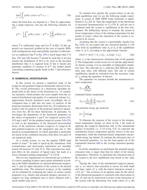
234101-8 Davidchack, Handel, and Tretyakov J. Chem. Phys. 130, 234101 2009 1 lim t t→ t0 Xs;xds = erg a . s ., 38 where the limit does not depend on x. Then by approximating a single trajectory, one gets the following estimator for erg , erg 1 T˜0 ˜ T Xs;xds ˇ erg ª 1 X¯ lh;x, L l=1 39 where T˜ is sufficiently large and Lh=T˜. In Ref. 23 this approach was rigorously justified in the case of ergodic SDEs with nondegenerate noise and globally Lipschitz coefficients. Let us emphasize that T˜ in Eq. 39 is much larger than T in Eqs. 35 and 36 because T˜ should be such that it not just ensures the distribution of Xt to be close to the invariant distribution like it is required from T but it should also guarantee smallness of variance of ˇ erg . See further details concerning computing ergodic limits in Ref. 7 and references therein. IV. NUMERICAL INVESTIGATION In this section we present a numerical study of the Langevin and gradient-Langevin thermostats derived in Sec. II. The overall performance of a thermostat algorithm depends both on the choice of the thermostat i.e., of continuous dynamics which produce the exact sample from the canonical distribution and quality of a numerical scheme i.e., approximate discrete dynamics used. Accordingly, the investigation here is split into two parts: i analysis of the proposed stochastic thermostats from Sec. II continuous dynamics and ii analysis of the proposed numerical integrators from Sec. III for these thermostats. In particular, we investigate the dependence of the thermostat properties on the choice of parameters and for Langevin system 12- 13 and and for the gradient-Langevin system 14-15, as well as the dependence of the numerical discretization errors of the numerical schemes Langevin A, Langevin B, and gradient-Langevin on the integration step size h. Our practical recommendations on which algorithm is preferable are based on the combined outcomes from these two parts of our numerical study. As a model system, we use the popular TIP4P rigid model of water. 11 In order to speed up the simulations, both Lennard-Jones and electrostatic interactions are smoothly turned off between 9.5 and 10 Å. This truncation has minimal effect on the structure of liquid water, but leads to a lower estimated melting temperature 24 of 219 K. The two key requirements of a thermostat are as follows: i correct sampling of phase space points distributed according to the Gibbs distribution at a desired thermostat temperature T, and ii rapid relaxation of the system to the desired equilibrium state. The numerical accuracy of the sampling can be estimated by comparing the values of various system properties e.g., kinetic and potential energies, pressure averaged over long simulation runs to those obtained with a much smaller step size h. L To estimate how quickly the system relaxes to the desired equilibrium state we use the following simple experiment. A system of 2000 TIP4P water molecules is equilibrated at T 0 =220 K. Then the temperature of the thermostat is increased instantaneously to T 1 =270 K, and the run is continued until the system is equilibrated at the new temperature. We deliberately choose to simulate the system at lower temperatures close to the melting temperature for this model of water, where the relaxation of the system is expected to be slower. Assuming that the system is exponentially ergodic see Eq. 34, we can expect that any measured quantity A will relax from its equilibrium value A 0 at T 0 to the equilibrium value A 1 at T 1 according to the approximate formula EAtAt A 1 + A 0 − A 1 exp− t/ A , 40 where A is the characteristic relaxation time of the quantity A. The temperature switch occurs at t=0 and the angle brackets denote average over an ensemble of independent simulation runs. The subscript on A indicates that different quantities may relax with different rates. The rate of system equilibration should be estimated from the maximum value of A among the quantities of interest. The quantities we measure include the translational kinetic temperature T tr = pT p 3nk B m , rotational kinetic temperature T rot = 2 3nk B n 3 l=1 j=1 V l q j , j , and potential energy per molecule U = 1 n Ur,q. 41 42 43 To illustrate the response of the system to the instantaneous temperature change, we show in Fig. 1 the result of applying the Langevin thermostat only to the translational degrees of freedom, i.e., =0 in Eq. 13. As expected, the translational kinetic temperature quickly relaxes to the new temperature, while the rotational kinetic temperature and potential energy lag behind. To estimate the relaxation rates of the measured quantities, we use the least-squares fit of the exponential function 40 to the average measured quantity At. In all the simulations we performed, the potential energy relaxation time is larger than that for either of the kinetic temperatures. Therefore, we determine the relaxation time of the system to the new equilibrium state based on the value of U . Varying the value of the translational Langevin parameter , we observe that relaxation is slower for both small and large values of , with the fastest relaxation around =4.0 ps −1 . The existence of an optimal value for the choice of the thermostat parameter is consistent with observations in Ref. 22 and can be understood in terms of the interaction of the system with the thermostat. For small values of , the Downloaded 12 Sep 2009 to 193.190.253.147. Redistribution subject to AIP license or copyright; see http://jcp.aip.org/jcp/copyright.jsp
234101-9 Langevin thermostat for rigid body dynamics J. Chem. Phys. 130, 234101 2009 280 2 270 260 1.8 10 3 γ,ps −1 T , K 250 240 230 1.6 1.4 U, kcal/mol 220 210 −10.4 −10.6 −10.8 −11 −11.2 −11.4 T tr (t) T rot (t) 0 5 10 15 20 Time, ps Γ, ps −1 10 2 10 1 10 0 10 0 10 1 10 2 1.2 1 0.8 0.6 0.4 0.2 0 τTtr, ps FIG. 1. Color online Relaxation dynamics with translational Langevin thermostat: =4.0 ps −1 , =0. Thin lines show relaxation dynamics averaged over ten independent runs, thick lines solid and dashed for translational and rotational temperatures, respectively show the least-squares fit to formula 40. The estimated values of the relaxation times are Ttr =0.2 ps, Trot =1.9 ps, and U =3.6 ps. relaxation of the system is slow due to the limited heat flux between the system and the thermostat. For large , even though the kinetic temperature relaxes very quickly, the relaxation of the configurational state of the system is apparently hindered by the disruptive influence of the random force on the Hamiltonian dynamics which is driving the system to the new equilibrium. A. Langevin thermostats Next, we investigate the dependence of the system relaxation time A on both and in Eqs. 12 and 13. In order to minimize the influence of the numerical discretization error, we use a relatively small time step of 0.2 fs. With such a small time step, the difference between Langevin A and Langevin B is negligible compared to the sampling error. To produce the results reported below, we use Langevin A. We evaluate U on a logarithmic grid of ranging from 0.2 to 300 ps −1 and ranging from 0.8 to 3000 ps −1 values using five independent runs at each point. The results are shown in Figs. 2–4. As expected, the relaxation speed of translational and rotational temperatures uniformly increases with increasing values of and , respectively. At the same time, the relaxation speed of the potential energy exhibits nonuniform dependence on the thermostat parameters. As can be seen in Fig. 4, the fastest relaxation of the system is achieved when the Langevin thermostat is applied to both translational and rotational degrees of freedom, with =2–8 ps −1 and =3–40 ps −1 . The relaxation dynamics of the system with the “optimal” choice of Langevin thermostat parameters is demonstrated in Fig. 5. In this case Ttr =0.28 ps, Trot =0.26 ps, and U =2.0 ps, which show that the system relaxation is almost twice as fast as when the Langevin thermostat is applied only to translational degrees of freedom. Note that the results shown in Fig. 4 for larger FIG. 2. Color online Translational temperature relaxation time for the Langevin thermostat 12-13 as a function of the thermostat parameters and . than about 100 ps −1 or larger than about 1000 ps −1 are not reliable due to excessive coupling of the system to the thermostat, which disrupts the Hamiltonian flow of the system. In this case, the relaxation dynamics is poorly represented by the exponential function 40 and thus the fits produce misleading values for the system relaxation time. In order to further investigate the properties of the Langevin thermostat, we have also computed the integrated autocorrelation time for the measured quantities of the system equilibrated at 270 K, where Γ, ps −1 ¯A =0 R A tdt, 10 3 10 2 10 1 10 0 γ,ps −1 10 0 10 1 10 2 0.25 0.2 0.15 0.1 0.05 FIG. 3. Color online Rotational temperature relaxation time for the Langevin thermostat 12-13 as a function of the thermostat parameters and . 0.3 0 τTrot ,ps Downloaded 12 Sep 2009 to 193.190.253.147. Redistribution subject to AIP license or copyright; see http://jcp.aip.org/jcp/copyright.jsp
Page 1 and 2: THE JOURNAL OF CHEMICAL PHYSICS 130
Page 3 and 4: 234101-3 Langevin thermostat for ri
Page 5 and 6: 234101-5 Langevin thermostat for ri
Page 7: 234101-7 Langevin thermostat for ri
Page 11 and 12: 234101-11 Langevin thermostat for r
Page 13 and 14: 234101-13 Langevin thermostat for r

Langevin thermostat for rigid body dynamics - Lammps

Create successful ePaper yourself

Delete template?

Save as template?