Proceedings - C-SRNWP Project
Proceedings - C-SRNWP Project
Proceedings - C-SRNWP Project

You also want an ePaper? Increase the reach of your titles
YUMPU automatically turns print PDFs into web optimized ePapers that Google loves.
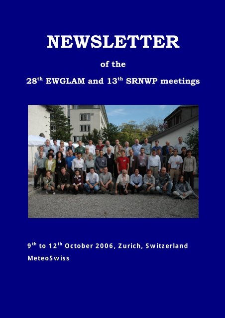
NEWSLETTER<br />
of the<br />
28 th EWGLAM and 13 th <strong>SRNWP</strong> meetings<br />
9 th to 12 th October 2006, Zurich, Switzerland<br />
MeteoSwiss
NEWSLETTER<br />
of the<br />
28 th EWGLAM and 13 th <strong>SRNWP</strong> meetings<br />
9 th to 12 th October 2006, Zurich, Switzerland<br />
MeteoSwiss
Newsletter of the 28th EWGLAM and 13th <strong>SRNWP</strong> meetings,<br />
9-12 October 2006, Zurich, Switzerland<br />
Editor Philippe A.J. Steiner, Federal Office of Meteorology and Climatology<br />
MeteoSwiss<br />
European Working Group on Limited Area Modelling, Meeting 28, Zurich,<br />
Switzerland<br />
Short-Range Numerical Weather Prediction, Meeting 13, Zurich, Switzerland<br />
ISBN 978-3-033-01152-6
Contents<br />
1 Introduction ...................................................................................................................... 5<br />
1.1 Foreword ....................................................................................................................6<br />
1.2 List of Partipicants ..................................................................................................... 7<br />
1.3 Programme ................................................................................................................. 9<br />
2 Consortia and ECMWF reports ................................................................................... 12<br />
2.1 ECMWF ................................................................................................................... 13<br />
2.2 ALADIN................................................................................................................... 22<br />
2.3 COSMO.................................................................................................................... 30<br />
2.4 HIRLAM .................................................................................................................. 42<br />
2.5 UKMO...................................................................................................................... 50<br />
3 National status reports................................................................................................... 58<br />
3.1 Belgium .................................................................................................................... 59<br />
3.2 Croatia ...................................................................................................................... 65<br />
3.3 Czech Republic ........................................................................................................ 69<br />
3.4 Denmark................................................................................................................... 72<br />
3.5 Estonia...................................................................................................................... 76<br />
3.6 Finland...................................................................................................................... 82<br />
3.7 France....................................................................................................................... 87<br />
3.8 Germany................................................................................................................... 92<br />
3.9 Hungary.................................................................................................................... 97<br />
3.10 Ireland..................................................................................................................... 103<br />
3.11 Italy......................................................................................................................... 108<br />
3.12 Netherlands............................................................................................................. 113<br />
3.13 Portugal .................................................................................................................. 122<br />
3.14 Romania ................................................................................................................. 128<br />
3.15 Slovakia.................................................................................................................. 134<br />
3.16 Slovenia.................................................................................................................. 139<br />
3.17 Spain....................................................................................................................... 144<br />
3.18 Sweden ................................................................................................................... 150<br />
3.19 Switzerland............................................................................................................. 154<br />
4 Scientific presentations on numerics and coupling numerics/physics..................... 160<br />
4.1 F. Vana: Dynamics & Coupling, ALADIN and LACE progress report for<br />
2005-2006............................................................................................................... 161<br />
4.2 J. Masek: Idealized tests of ALADIN-NH dynamical kernel at very high<br />
resolution................................................................................................................ 168<br />
5 Scientific presentations on data assimilation............................................................. 179<br />
5.1 C. Schraff: COSMO: Overview and Strategy on Data Assimilation for LM ........ 180<br />
5.2 D. Leuenberger et al.: The Latent Heat Nudging Scheme of COSMO.................. 187<br />
5.3 C. Fischer and A. Horanyi: Aladin consortium activities in data assimilation ...... 193<br />
5.4 G. Bölöni: Data assimilation activities in LACE 2006-2007................................. 202<br />
6 Scientific presentations on physics.............................................................................. 207<br />
6.1 M. Bush: Physics improvements in the NAE model, dust forecasting,<br />
firefighting and chemistry ...................................................................................... 208<br />
3
6.2 P. Clark et al.: The Convective-Scale UM: Current Status, Verification and<br />
Physics Developments............................................................................................ 221<br />
6.3 S. Tijm: HIRLAM Physics developments.............................................................. 232<br />
6.4 S. Gollvik: Snow, forest and lake aspects in the Hirlam surface scheme .............. 238<br />
6.5 N. Pristov et at.: ALARO-0 Physics developments at LACE in 2006................... 248<br />
7 Scientific presentations on predictability and EPS ................................................... 257<br />
7.1 Y. Wang: LAMEPS Development of ALADIN-LACE......................................... 258<br />
7.2 J. García-Moya et al.: Recent Experiences with the INM Multi-model EPS<br />
scheme.................................................................................................................... 267<br />
7.3 C. Marsigli et al.: The COSMO SREPS project .................................................... 277<br />
7.4 P. Eckert: COSMO ensemble systems ................................................................... 284<br />
8 EWGLAM final discussion.......................................................................................... 290<br />
9 <strong>SRNWP</strong> business meeting report................................................................................ 293<br />
4
1 Introduction<br />
5
1.1 Foreword<br />
In 2006, MeteoSwiss had the pleasure to organise and host the 28th meeting of the European<br />
Working Group on Limited Area Modelling (EWGLAM) and the 13 th meeting of the<br />
EUMETNET Programme Short-Range Numerical Weather Prediction (<strong>SRNWP</strong>). They took<br />
place from the 9 th to the 12 th of October, 2006, in Zurich. I want to warmly thank all the<br />
colleagues of MeteoSwiss involved in the organisation and all the participants; they have so<br />
well contributed to the success of the meetings.<br />
The meetings were for the first time held in the new format, defined in the 2005 meetings in<br />
Ljubljana, with the target to better allow the decision making for enhanced collaboration. A<br />
more formalised and extended presentation of the recent developments of the consortia has<br />
been introduced in the EWGLAM part enabling a discussion between leaders of the four<br />
areas: data assimilation, numerics & coupling numerics/physics, physics, predictability &<br />
EPS. In the <strong>SRNWP</strong> part, the reports of the lead centres have been replaced by a discussion of<br />
the new EUMETNET programme to replace <strong>SRNWP</strong> after 2007. The new format has very<br />
well passed its first trial and all agreed to keep it for the next meetings planed in Dubrovnik in<br />
October 2007.<br />
In this Newsletter, you will find after the program and the list of participants, the reports of<br />
ECMWF and of the consortia, the national status reports and the scientific contributions<br />
grouped by area and at the end the minutes of the EWGLAM final discussion as well as the<br />
report of the <strong>SRNWP</strong> session.<br />
Zurich, February 2007<br />
Philippe Steiner<br />
6
1.2 List of Partipicants<br />
Marco Arpagaus MeteoSwiss Switzerland<br />
Jean-Marie Bettems MeteoSwiss Switzerland<br />
Gergely Bölöni Hungarian Meteorological Service Hungary<br />
Massimo Bonavita CNMCA Italy<br />
Mike Bush Met Office United Kingdom<br />
Gerard Cats KNMI Netherlands<br />
Jean-Pierre Chalon EUMETNET France<br />
Guy de Morsier MeteoSwiss Switzerland<br />
Terry Davies Met Office United Kingdom<br />
Maria Derkova Slovak Hydrometeorogical Institute Slovakia<br />
Pierre Eckert MeteoSwiss Switzerland<br />
Claude Fischer Météo-France France<br />
Richard Forbes Met Office United Kingdom<br />
Carl Fortelius Finnish Meteorological Institute Finland<br />
Jean-François Geleyn Czech Hydrometeorological Institute Czech Republic<br />
Stefan Gollvik SMHI Sweden<br />
Nils Gustafsson SMHI Sweden<br />
James Hamilton Met Éireann Ireland<br />
Andras Horanyi Hungarian Meteorological Service Hungary<br />
Mariano Hortal ECMWF England<br />
Tamara Ivanova LVGMA Latvia<br />
Stjepan Ivatek-Sahdan Meteorological & Hydrological Service Croatia<br />
Trond Iversen Norwegian Meteorological Institute Norway<br />
Dijana Klaric Meteorological & Hydrological Service Croatia<br />
Daniel Leuenberger MeteoSwiss Switzerland<br />
Bruce Macpherson Met Office United Kingdom<br />
Aarne Männik University of Tartu Estonia<br />
Chiara Marsigli ARPA-SIM Italy<br />
Jan Masek Slovak HydroMeteorological Institute Slovakia<br />
Jean-Antoine Maziejewski Météo-France France<br />
Lars Meuller SMHI Sweden<br />
Dmitrii Mironov Deutscher Wetterdienst Germany<br />
Maria José Monteiro Instituto de Meteorologia Portugal<br />
Mark Naylor Met Office United Kingdom<br />
Jeanette Onvlee KNMI Netherlands<br />
Bartolome Orfila Instituto Nacional de Meteorología Spain<br />
Tiziana Paccagnella ARPA-SIM Emilia-Romagna Italy<br />
Ioannis Papageorgiou Hellenic National Meteorological Service Greece<br />
Jean-Marcel Piriou Meteo-France France<br />
Patricia Pottier Météo-France France<br />
Neva Pristov Environmental Agency of the Republic of Slovenia Slovenia<br />
Jean Quiby EUMETNET Switzerland<br />
Bent Sass Danish Meteorological Institute Denmark<br />
Francis Schubiger MeteoSwiss Switzerland<br />
Jan-Peter Schulz Deutscher Wetterdienst Germany<br />
Harald Seidl Central Institute for Meteorology and Geodynamics Austria<br />
7
Cornel Soci National Meteorological Administration Romania<br />
Philippe Steiner MeteoSwiss Switzerland<br />
Jürgen Steppeler Deutscher Wetterdienst Germany<br />
Sander Tijm KNMI Netherlands<br />
Martina Tudor Meteorological & Hydrological Service Croatia<br />
Per Unden SMHI Sweden<br />
Filip Vana Czech Hydrometeorological Institute Czech Republic<br />
Josette Vanderborght Institut Royal Météorologique Belgique<br />
André Walser MeteoSwiss Switzerland<br />
Xiaohua Yang Danish Meteorological Institute Denmark<br />
8
1.3 Programme<br />
Monday, 9th October 2006<br />
8:15 – 8:45 Registration<br />
9:00 Opening by the Director of MeteoSwiss, D. Keuerleber and organisational matters<br />
09:15 – 11:30 Presentation of the Consortia and ECMWF chair: Marco Arpagaus<br />
09:15 – 09:30 Tiziana Paccagnella COSMO<br />
09:30 – 09:45 Mike Bush UK Met Office<br />
09:45 – 10:00 Jeanette Onvlee HIRLAM<br />
10:00 – 10:15 Jean-François Geleyn ALADIN<br />
10:15 – 10:30 Dijana Klaric LACE<br />
10:30 – 11:00 Coffee break<br />
11:00 – 11:30 Mariano Hortal ECMWF<br />
11:30 – 14:45 Presentations of national posters chair: Per Unden<br />
Harald Seidl<br />
Austria<br />
Josette Vanderborght<br />
Belgium<br />
Stjepan Ivatek-Sahdan<br />
Croatia<br />
Filip Vana<br />
Czech Republic<br />
Bent Sass<br />
Denmark<br />
Aarne Männik<br />
Estonia<br />
Carl Fortelius<br />
Finland<br />
Claude Fischer<br />
France<br />
Jan-Peter Schulz<br />
Germany<br />
Andras Horanyi<br />
Hungary<br />
12:30 – 13:45 Lunch break<br />
James Hamilton<br />
Massimo Bonavita<br />
Gerard Cats<br />
Maria José Monteiro<br />
Cornel Soci<br />
Maria Derkova<br />
Neva Pristov<br />
Bartolome Orfila<br />
Lars Meuller<br />
Philippe Steiner<br />
Mike Bush<br />
14:45 – 15.15 Poster session<br />
Ireland<br />
Italy<br />
Netherlands<br />
Portugal<br />
Romania<br />
Slovakia<br />
Slovenia<br />
Spain<br />
Sweden<br />
Switzerland<br />
United Kingdom<br />
15:15 – 15:45 Coffee break<br />
15:45 – 17:45<br />
Scientific presentations on numerics and<br />
coupling numerics/physics<br />
Chair: Claude Fischer<br />
15:45 – 16:15 Terry Davies<br />
Lateral boundary conditions, variable resolution or<br />
both?<br />
9
16:15 – 16:45 Filip Vana general Dynamics status in ALADIN and LACE<br />
16:45 – 17:00 Jürgen Steppeler Overview and strategy on numerics. The LMZ_<br />
including coupling Numerics & Physics<br />
17:00 – 17:30 Jan Masek Idealised test of ALADIN NH dynamical core at very<br />
high resolution (and comparison of hydrostatic and<br />
NH versions)<br />
17:30 – 17:45 All Discussion<br />
18:30 City tour (start at hotel Basilea) with optional dinner<br />
Tuesday, 10th October<br />
08:30 – 11:50 Scientific presentations on data assimilation Chair: Terry Davies<br />
08:30 – 09:00 Nils Gustafsson Recent results and plans for HIRLAM 4D-VAR<br />
09:00 – 09:15 Jürgen Steppeler Overview and strategy on data assimilation for LM<br />
09:15 – 09:45 Bruce Macpherson Assimilation developments in North Atlantic and<br />
UK models<br />
09:45 – 10:00 Mark Naylor Aspects of 4DVAR in North Atlantic model<br />
10:00 – 10:30 Coffee break<br />
10:30 – 10:45 Daniel Leuenberger The LHN scheme of COSMO<br />
10:45 – 11:15 Claude Fischer & An- Data assimilation - ALADIN<br />
dras Horanyi<br />
11:15 – 11:35 Gergely Bölöni Data assimilation – LACE specific<br />
11:35 – 11:50 All Discussion<br />
11:50 – 13:30 Lunch break with optional visit of the forecast service<br />
Chair: Tiziana<br />
13:30 – 17:30 Scientific presentations on Physics<br />
Paccagnella<br />
13:30 – 14:00 Jean-Marcel Piriou Parametrisation in ALADIN<br />
14:00 – 14:15 Marco Arpagaus Overview and strategy on LM Physics<br />
14:15 – 14:30 Dmitrii Mironov The UTCS <strong>Project</strong><br />
14:30 – 15:00 Mike Bush Physics improvements in the North Atlantic Model<br />
15:00 – 15:30 Coffee break<br />
15:30 – 16:00 Richard Forbes Recent results from parametrization developments<br />
in the convective-scale (~1 km) Unified Model<br />
16:00 – 16:30 Sander Tijm Physics developments in HIRLAM-A<br />
16:30 – 16:55 Stefan Gollvik Snow, forest and lake aspects in the HIRLAM<br />
surface scheme<br />
16:55 – 17:15 Neva Pristov ALARO part developed at LACE<br />
17:15 – 17:30 All Discussion<br />
18:00 Apero offered by MeteoSwiss on the occasion of its 125th anniversary<br />
10
08:30 – 11:00<br />
Wednesday, 11th October<br />
Scientific presentations on predictability and<br />
EPS<br />
Chair: Andras Horanyi<br />
08:30 – 09:00 Harald Seidl LAMEPS Development and Plan of ALADINLACE<br />
09:00 – 09:20 Trond Iversen<br />
09:20 – 09:45 Bartolome Orfila<br />
A proposal for Grand Limited Area Model Ensemble<br />
Prediction System (GLAMEPS)<br />
Recent experiences with the INM multi-model EPS<br />
scheme<br />
09:45 – 10:00 Chiara Marsigli The COSMO SREPS project<br />
10:00 – 10:30 Coffee break<br />
10:30 – 10:45 Pierre Eckert COSMO ensemble systems<br />
10:45 – 11:00 All Discussion<br />
11:00 – 11:30 EWGLAM Final Discussion<br />
-Preparation of the newsletters -Date and place<br />
of the next meeting (2007)<br />
-Place of the meeting 2008 (tentative)<br />
Chair: Stjepan Ivatek-<br />
Sahdan<br />
11:30 – 12:00 <strong>SRNWP</strong> business meeting Chair: Jean Quiby<br />
12:30 Excursion and offered dinner<br />
09:00 – 13:00<br />
Thursday, 12th October<br />
10:30 – 11:00 Coffee break<br />
Discussion of the 3rd phase (from 1st January<br />
2008) of the <strong>SRNWP</strong> Programme<br />
Chair: Jean Quiby<br />
-Introduction to the NWP vision -draft “Programme Proposal” and “Programme<br />
Decision” -Procedure for the elaboration of a larger <strong>SRNWP</strong> scientific project<br />
-Other proposals identified ad the Vision Workshop: -Common format for the<br />
product exchange -NWP requirements for next phase of EUMETNET obs pgm -<br />
Procedure for the prioritization of the proposals from the Vision Workshop -Work<br />
plan/timeline for programme proposal until spring Council<br />
13:00 End of the meetings<br />
11
2 Consortia and ECMWF reports<br />
12
2.1 ECMWF<br />
13
Research Progress at ECMWF 2005-2006<br />
Mariano Hortal<br />
The highlights of the activity at ECMWF during the last year have been:<br />
• Cycle 30r1 of the IFS went into operations on February the 1 st , after extensive pre-operational<br />
testing (more than 300 days). It included resolution upgrades to T799 in the horizontal and 91<br />
levels in the vertical (with the top of the model raised to 0.01 hPa) for both the<br />
deterministic forecast and the outer loops of 4D-Var, T255 horizontal resolution in the<br />
second minimization of 4D-Var (the first minimization stayed at T95), and T399 with 62<br />
levels for the Ensemble prediction system (EPS).<br />
• Cycle 31r1 of the IFS, including significant upgrades of the model physics, a variational<br />
bias correction scheme and the variable-resolution EPS (VAREPS) was made operational<br />
on September the 12 th . The physics upgrades produce a significant improvement of the<br />
model’s climate and planed upgrades of the radiation parameterization will improve that<br />
further.<br />
• The ERA-interim production has started.<br />
• The cycle 31r1 of the IFS is now used for the deterministic model, the 4D-Var, the EPS, the<br />
seasonal forecast, the ERA-interim and the OSSE (observation systems simulation<br />
experiments) nature runs, in line with the strategy objective of increase efforts towards a<br />
fully unified ensemble system.<br />
Unfortunately, due to budget cuts, two research positions (one in Numerical Aspects and the<br />
other in Seasonal Forecasts) are now frozen.<br />
Ensemble Prediction System (EPS)<br />
On February 1 st the resolution of the EPS forecast model was increased to T399L62, as a first<br />
step towards the variable-resolution EPS (VAREPS) whose second phase was implemented<br />
on September 12 th . The singular vectors for the initial perturbations are computed with a<br />
T42L62 resolution.<br />
In the second phase towards the full VAREPS, the first 10 days of the ensemble are run at a<br />
resolution of T399. Then the day-9 forecast is interpolated to T255 resolution and run to day<br />
15 at that resolution. The 1-day overlap allows the model to settle down at the new resolution.<br />
The third phase of the implementation, planned to become operational in 2007, will be to<br />
extend, once per week, the forecasts to one month, including coupling with the ocean.<br />
The VAREPS system aims to provide a better prediction of small-scale, severe-weather<br />
events in the early forecast range, and skilful large-scale guidance in the medium forecast<br />
range.<br />
The performance of the EPS since the resolution increase has been very good.<br />
For verification purposes, a new climatology of each day of the year has been compiled using<br />
ERA-40 analyses. The use of the new climatology for the operational 2005 forecasts tends to<br />
reduce the ACC of Z500, in particular for months with ACC lower than 70%.<br />
14
The impact of a stochastic representation of unresolved processes on systematic model error<br />
was assessed using a) a cellular automaton stochastic backscatter scheme (CASBS) and b) a<br />
stochastic-super-cluster (SSC) scheme run at T L 95L60 for 40 winters. The CASBS improves<br />
blocking (see Fig 1), reduces the systematic error over the North Pacific and greatly improves<br />
the precipitation in the tropics. The SSC scheme aims at representing the dynamical signature<br />
of organised convection in a stochastic manner and is only active in the tropical band. First<br />
results indicate that the introduction of the signature of cloud-super-clusters not only<br />
improves tropical precipitation but more importantly increases the activity of the model in the<br />
MJO-band of 30-60 days.<br />
Fig 1. Mean blocking frequency (Tibaldi and Molteni index) over the Northern<br />
Hemisphere in winter (DJFM, 1-month lead time) for control (red), CASBS (blue) and<br />
ERA40 (black)<br />
Montly and seasonal forecasts<br />
During the past year, several model changes have taken place. In June 2005, Cycle CY29R2<br />
was implemented and a new sea-ice treatment was introduced. Now the sea-ice is persisted<br />
until day 10, and then relaxed to climatology until day 30. After day 30, climatological sea-ice<br />
from ERA40 is used. In February 2006, cycle CY30R1 was introduced, with a new vertical<br />
resolution for the atmospheric part: T L 159L62 instead of T L 159L40. Hindcast experiments<br />
suggest that those changes had no significant impact on the probabilistic scores of the<br />
monthly forecasting system over the Northern Hemisphere.<br />
During the development of System 3 for monthly forecasts various versions of the<br />
atmospheric model were tested, both in the medium-range system and in the seasonal system,<br />
culminating in the creation of cycle 31r1. Tests of this model version suggest that it is the best<br />
cycle to date in terms of SST anomaly forecasts, and that the model climate has also<br />
improved. It was therefore adopted for System 3.<br />
Re-forecasts using this new system 3 are now in production and the first operational forecast<br />
using this system should be in January 2007.<br />
Following the users’ request, System 3 forecasts will be 7 months long rather than 6 months.<br />
Additionally, once per quarter a modest ensemble will be run to 13 months, in order to give<br />
an “ENSO outlook”.<br />
A new ocean analysis system has been developed to provide initial conditions for S3 and for<br />
monthly forecasts. It consists of an ocean re-analysis and a real time ocean analysis. The<br />
15
ocean data assimilation system for S3 is based on HOPE-OI, as in the previous system (S2),<br />
but major upgrades have been introduced.<br />
Initial results of the ENSEMBLES project show that the multi-model approach to monthly<br />
and seasonal forecasts is still the most skilful one but a better stochastic physics treatment can<br />
improve significantly several aspects.<br />
Numerical Aspects<br />
1) The high resolution system T799L91 & T399L62 EPS (IFS Cycle 30R1) which had<br />
undergone extensive pre-operational testing during 2005 became operational on February 1 st<br />
2006. A total of ten months of assimilation-forecast experimentation were run with Cycle<br />
30R1, four months (1 October 2005 to 31 January 2006) in e-suite mode by the Operations<br />
Department and six months by the Research Department. Better representation of the<br />
orography and increased vertical resolution lead to more observations being accepted in the<br />
analysis. The mean scores are in general better than the control scores with T511L60 and<br />
Cycle 29R2, with the largest gain and highest statistical significance in the southern<br />
hemisphere.<br />
Table 1 summarizes the statistical significance obtained with the t-test for Z500 scores for the<br />
northern hemisphere, southern hemisphere and for Europe. Numbers in green mean the high<br />
resolution system T799L91 (Cycle 30R1) is better than T511L60 (Cycle 29R1) with a<br />
statistical significance given by the value. Smaller values mean higher statistical significance.<br />
The sample size is 311 forecasts.<br />
Area Score Day<br />
2<br />
Day<br />
3<br />
2%<br />
0.1%<br />
0.1%<br />
0.1%<br />
-<br />
2%<br />
Day<br />
5<br />
-<br />
10%<br />
0.1%<br />
0.1%<br />
2%<br />
10%<br />
Day<br />
7<br />
-<br />
-<br />
0.1%<br />
0.1%<br />
-<br />
5%<br />
N<br />
Hem.<br />
S Hem.<br />
AC<br />
RMSE<br />
AC<br />
RMSE<br />
AC<br />
RMSE<br />
0.1%<br />
0.1%<br />
0.1%<br />
0.1%<br />
-<br />
0.5%<br />
Europe<br />
2) Development of a non-interpolating version of the semi-Lagrangian advection.<br />
The quality of the semi-Lagrangian advection scheme depends on the quality of the<br />
interpolations to the departure points of the trajectories. In the operational configuration,<br />
cubic Lagrange interpolations with quasi-monotone limiters are used for the advected<br />
quantities and linear interpolations are used for the right-hand side of the equations.<br />
An alternative to more accurate interpolation to improve the quality of the semi-Lagrangian<br />
advection may be a “non-interpolating version” that does not require interpolations at the<br />
departure point. A non-interpolating algorithm in three dimensions has been coded. The<br />
nearest grid point to the semi-Lagrangian departure point is found and the semi-Lagrangian<br />
method is applied with this point as departure point, while the remaining or “residual”<br />
advection is performed in an Eulerian way. As part of the research process, a “noninterpolating<br />
in the vertical only” version has also been coded. Finite-elements in the vertical<br />
16
0.2 10 -6<br />
are used for computing accurate vertical derivatives for the residual advection. Several<br />
options for treating the residual advection of the scheme have been coded and will be<br />
compared. This non-interpolating semi-Lagrangian scheme is expected to have less damping<br />
of the smallest scales than the operational scheme, and hence produce a more realistic kinetic<br />
energy spectrum.<br />
3) Fast Legendre transform algorithm<br />
The Legendre transforms of our spectral model is the part of the model which runs most<br />
efficiently. It is therefore not clear yet at which horizontal resolution the advantage of a<br />
smaller number of computations in a fast Legendre transform algorithm will overcome the<br />
loss of efficiency stemming from not being a pure matrix-multiply operation. This together<br />
with the fact that a position of the Numerical Aspects Section has been frozen due to cuts in<br />
the budget has made this work a low-priority work.<br />
4) Dynamics and physics run at different horizontal resolutions.<br />
The possibility of running the dynamics and the physics at different resolutions has been<br />
introduced in the forecast model. Preliminary results indicate that the verification scores, for a<br />
given dynamics resolution, degrade progressively as the physics resolution coarsens and<br />
become better when the resolution of the physics increases. More work is needed in order to<br />
check other aspects of the runs such as the influence on the model climate.<br />
5) The improvement in the efficiency of the forecast model when using the Symmetric<br />
Multi Threading (SMT) capability of the processors of the new IBM computer has been<br />
realized, the efficiency becoming 13% of the peak speed instead the 7% achieved with the<br />
previous machine.<br />
6) Non-hydrostatic dynamics in the IFS<br />
In collaboration with Météo-France, the non-hydrostatic version developed by the ALADIN<br />
group has been implemented in the global IFS/ARPEGE model and interfaced with the<br />
ECMWF physics.<br />
Work in collaboration with ALADIN and HIRLAM will be carried out to implement a finiteelement<br />
discretization in the vertical.<br />
Some experiments have been run using idealized conditions which expose the non-hydrostatic<br />
effects and compared with a reference non-hydrostatic model supplied by NCAR. Fig 2 shows<br />
cross-sections of the horizontal divergence in model runs with only a bell-shaped mountain<br />
and the stability parameter NL/U (where N is the Brünt-Väisalä frequency, L the length-scale<br />
of the mountain and U the constant background zonal wind) set to a value of 5 to expose nonhydrostatic<br />
effects.<br />
0.01<br />
0.02<br />
0.03<br />
0.05<br />
0.07<br />
0.1<br />
0.2<br />
0.3<br />
0.5<br />
0.7<br />
1<br />
2<br />
3<br />
5<br />
7<br />
10<br />
20<br />
30<br />
50<br />
70<br />
100<br />
200<br />
300<br />
500<br />
700<br />
1000<br />
0.1 10 -6 0.1 10 -6<br />
0.01<br />
0.02<br />
0.03<br />
0.05<br />
0.07<br />
0.1<br />
0.2<br />
0.3<br />
0.5<br />
0.7<br />
1<br />
2<br />
3<br />
5<br />
7<br />
10<br />
20<br />
30<br />
50<br />
70<br />
100<br />
200<br />
300<br />
500<br />
700<br />
150 O W 100 O W 50 O W 0 O 50 O E 100 O E 150 O E<br />
1000<br />
150<br />
16.5N<br />
O W 100 O W 50 O W 0 O 50 O E 100 O E 150 O E<br />
16.5N<br />
0.6 10 -6<br />
0.4 10 -6<br />
0.2 10 -6<br />
Fig 2. Cross-section of the horizontal divergence near a bell-shaped mountain using the<br />
hydrostatic (left) and the non-hydrostatic (right) versions of the IFS model.<br />
17<br />
0.2 10 -6<br />
0.2 10 -6<br />
0.2 10 -6<br />
0.2 10 -6<br />
-0.2 10 -6<br />
-0.2 10 -6<br />
0.2 10 -6<br />
0.2 10 -6<br />
0.2 10 -6 0.2 10 -6<br />
0.2 10 -6<br />
-0.4 10 -6<br />
-0.4 10 -6<br />
0.4 10 -6<br />
-0.2 10 -6<br />
-0.2 10 -6
Physical Aspects<br />
1) The introduction of cycle 31r1 involves a substantial number of changes in the<br />
parametrized physics:<br />
• Changes in the cloud scheme related to ice sedimentation, treatment of ice super-saturation<br />
and the conversion to snow.<br />
• Implicit computation of all convective transports.<br />
• Introduction of the turbulent orographic form drag scheme (TOFD) to replace the effective<br />
roughness length concept, exclusion of the blocked layer in the forcing of gravity waves<br />
(cut-off mountain), and a combined implicit computation of turbulence, TOFD and subgrid<br />
orographic drag.<br />
• The wind gust parametrization (for post processing only) has a revised numerical treatment<br />
which behaves better over orography and solves to a large extent the adverse interaction<br />
with stochastic physics of the previous implementation.<br />
• Air/sea interaction assumes 98% relative humidity at the ocean surface instead of 100% to<br />
account for ocean salinity. Apart from cool skin and warm layer effects (which are included<br />
in the code but not activated), this change brings the ECMWF scheme close to the<br />
TOGA/COARE algorithm (Fairall et al. 1996) and results in a minor reduction of latent<br />
heat flux over the ocean.<br />
• The linear convection model, as used in the assimilation of rain-affected radiances, has<br />
been improved.<br />
The model changes improve physical realism (e.g. ice super saturation, salinity effects on<br />
evaporation) and most of these changes are necessary for further development (e.g. TOFD to<br />
allow work on atmosphere/vegetation exchange, implicit convection for numerical stability).<br />
The impact is very positive on the tropical climate of the model which is clearly reflected in<br />
radiation at the top of the atmosphere and in upper tropospheric winds. The impact on<br />
medium range forecasts is mainly neutral except for some seasonal dependent positive signals<br />
related to the surface drag over land and orographic effects.<br />
2) New radiation scheme<br />
A new version of the short-wave part of the radiation scheme RRTM is being developed. This<br />
version uses the “Monte-Carlo independent column approximation” for the cloud overlap and<br />
new cloud radiative properties. More work is needed to reduce the cost of the scheme which<br />
uses 112 spectral intervals and increases the cost of the forecast model by 30%.<br />
The scheme improves dramatically the radiative forcing in the model leading to an improved<br />
climate.<br />
3) New version of the linearized moist physics<br />
The use of the new moist physics in the high-resolution minimization part of 4D-Var leads to<br />
a larger decrease in the cost function. The influence on the verification scores over the<br />
Northern Hemisphere is slightly positive but it improves substantially the scores over North<br />
America in winter.<br />
Work has started on the tangent-linear and adjoint of the surface parameterization.<br />
4) New soil hydrology H-TESSEL<br />
The new scheme uses a recent digital soil map of the world and shows an improved match to<br />
soil temperature observations with respect to the previous scheme TESSEL.<br />
18
Ocean waves<br />
The resolution of the European wave model will increase shortly.<br />
An algorithm for retrieving wind from altimeter data has been developed at ECMWF and<br />
adopted operationally by ESA.<br />
Data assimilation<br />
Experimentation with three outer loops at T799 is in progress using inner loop resolutions of<br />
T95/T159/T255 and the new linear physics. The forecast skill is improved with this setup but<br />
the cost is incompatible with operational delivery times and needs further optimization.<br />
A weak constraint 4D-Var is being developed in order to account for model error in the<br />
assimilation which will allow the use of longer assimilation windows. At the present moment,<br />
the skill of a 12h weak constraint 4D-Var (using two 6-h windows) is lower that the<br />
operational 12-h window 4D-Var.<br />
The ensemble data assimilation system is being further developed. The system will allow an<br />
easier J b recalibration. Future work in the system includes the generation of flow-dependent<br />
background error variances and defining optimal perturbations to observations, with due<br />
representation of observation error correlations.<br />
Including observation error correlations in the assimilation: an approximation is to use blockdiagonal<br />
matrices with groups of intercorrelated data (observations of the same category).<br />
Another possibility which will be explored is to use an approximation based on a truncated<br />
eigenvector representation of the correlation matrices.<br />
Surface data assimilation system (SDAS): An Extended Kalman Filter method, based on the<br />
experience gained during ELDAS is being developed.<br />
The principle of the method is to adjust the initial soil moisture content to minimize the<br />
differences between observations and model-equivalent for soil-moisture related quantities<br />
during a 24-hour window.<br />
In addition to soil moisture and temperature, the SDAS development version also treats the<br />
snow cover, the SST and the sea-ice.<br />
Other work in data assimilation includes a better coupling between temperature and humidity<br />
during the assimilation process and better interpolation of the high-resolution trajectory to the<br />
lower resolution of the inner loops of 4D-Var.<br />
Satellite Data<br />
Several modifications to the first operational version of the 1D+4D-Var assimilation of rainaffected<br />
passive microwave radiometer data from SSMI have been introduced in cycle 31r1 of<br />
the IFS.<br />
Development of the variational bias correction system (VARBC) for satellite radiances has<br />
reached maturity. The scheme has demonstrated an ability to distinguish between systematic<br />
errors in the observations (or observation operators) and the assimilating model. Corrections<br />
generated by the adaptive scheme have been implemented statically in operations in February<br />
2006, significantly improving the fit of the assimilation system to radiosonde temperature<br />
data in the lower stratosphere. Implementation of the fully evolving VARBC system is<br />
undergoing final pre-operational testing as part of IFS cycle 31r1 and is performing well.<br />
Developments for the assimilation of emitted infrared limb radiances from MIPAS have been<br />
completed as part of the EU-funded ASSET project. MIPAS radiances can now be assimilated<br />
19
either with a 1-dimensional observation operator which assumes local horizontal homogeneity<br />
for the radiative transfer calculations, or with a 2-dimensional observation operator which<br />
takes into account horizontal gradients along the limb-viewing plane.<br />
The first set of experiments assimilating CHAMP GPS radio occultation (GPSRO)<br />
measurements with 2-dimensional bending angle observation operators has been completed.<br />
The 2-dimensional operators improved the bending angle departure statistics in the lower<br />
troposphere by around ~5% compared with a 1-dimensional bending angle operator, although<br />
this did not translate into a clear, statistically significant improvement in the forecast scores.<br />
COSMIC data (which has been seen to be of high quality) have been received from August<br />
and should be used in operations soon.<br />
Green dots – COSMIC GPSRO locations over a 24 hour period. Red dots: radiosondes<br />
Observing System Experiments (OSEs) coordinated by EUCOS have been performed to<br />
examine the various components of the terrestrial Observing System, in the presence of the<br />
current satellite-based Observing System. Results from a summer period (46 days) are<br />
currently being assessed. The winter studies indicate a large impact of the radiosondes (wind<br />
and temperature) and aircraft (wind and temperature), a marginal impact of radiosonde<br />
humidity information, and a contrasted impact (with negative spells) from the wind profilers.<br />
REANALYSIS<br />
The ERA-interim reanalysis has started. It covers the period from 1989 and will be continued<br />
in near-real time when it reaches the present (“climate data assimilation mode”).<br />
• It uses Cycle 31r1 of the IFS 12-hour window 4D-Var and T255 resolution in the outer<br />
loops. Currently two versions exist: 60 and 91 levels. Only the best version will be<br />
continued in near-real time.<br />
• The set of observations and SST/ice information used is the same as in ERA-40 until 2002,<br />
then operational datasets will be used.<br />
• It also uses Meteosat AMV´s reprocessed by Eumetsat and ERS-1 and ERS-2 altimeter and<br />
scatterometer data reprocessed by ESA.<br />
• It uses 1dVar+4dvar assimilation of rain-affected SSMI radiances.<br />
• It uses variational bias correction of all clear sky satellite radiances and automated bias<br />
correction for surface pressure observations.<br />
20
• Special attention currently paid to the behaviour of the VarBC scheme.<br />
• It uses radiosonde homogenization and improved bias correction tables.<br />
• Most problems identified in ERA-40 have been solved.<br />
Mean curves<br />
850hPa Vector Wind<br />
Root mean square error forecast<br />
Tropics Lat -20.0 to 20.0 Lon -180.0 to 180.0<br />
Date: 19890101 12UTC to 19901216 12UTC<br />
Mean calculation method: standard<br />
Population: 48,48,48,48,48,48,48,48,48,48,48,48,48,48,48,48,48,48,48,48 (averaged)<br />
6<br />
5.5<br />
5<br />
4.5<br />
4<br />
3.5<br />
3<br />
2.5<br />
2<br />
1.5<br />
1<br />
0.5<br />
oper<br />
ERA-15 aer15<br />
ERA-40 0256<br />
ERA-Interim a0060 test<br />
1 2 3 4 5 6 7 8 9 10<br />
Forecast Day<br />
21
2.2 ALADIN<br />
22
ALADIN: now a Programme; with a new governance;<br />
with new emphases; and with “HARMONIE” as<br />
background<br />
J.-F. Geleyn<br />
CHMI & Météo-France<br />
ALADIN Programme Manager<br />
Introduction<br />
Since the last EWGLAM/<strong>SRNWP</strong> meeting of 2005, many changes happened within the scope<br />
of the ALADIN Consortium. What was still implicitly considered as a <strong>Project</strong>, fourteen years<br />
after its effective launching, became a Programme at the occasion of the signature by 15<br />
Partners (Algeria, Austria, Belgium, Bulgaria, Croatia, Czech Republic, France, Hungary,<br />
Morocco, Poland, Portugal, Romania, Slovakia, Slovenia, Tunisia) of the third ALADIN<br />
Memorandum of Understanding (MoU3) on 21/10/05 in Bratislava. This MoU3 differs<br />
significantly from the two previous ones:<br />
• The ‘Programme’ aspects are (i) a clearer definition of Membership and of the conditions<br />
of accession to the status of full Membership, (ii) the establishment of a basic budgetary<br />
procedure (with the previously existing efforts of Météo-France and RC LACE continuing<br />
independently) and (iii) a completely new governance, the details of which shall be listed<br />
now.<br />
• The ALADIN General Assembly (GA) keeps its composition and decision role, but it gets a<br />
stable Chairmanship.<br />
• There is now a Policy Advisory Committee (PAC), that meets once or twice a year.<br />
• Each Partner must identify a Local Team Manager (LTM) with a reinforced amount of<br />
rights and duties for the day to day progress of the Programme.<br />
• There is a Programme Manager (PM) for the overall coordination of planned actions as<br />
well as for the contacts with the Chair of the GA, the PAC, RC LACE, the specific features<br />
happening in Toulouse and HIRLAM.<br />
• The PM gets assistance from both a Committee for Scientific and System Issues (CSSI,<br />
structured by topics) and a Support Team (structured by type of tasks).<br />
In a nutshell, the three issues that the new structure/governance gave priority to within the<br />
past twelve months were:<br />
• Establishing a better ‘transversal support to operations’ in order to save manpower and to<br />
streamline some previously non-codified aspects.<br />
• Finding a clearer definition for the links between the AROME and ALARO sub-projects<br />
(see Part II).<br />
• Kicking off the collection and use of the central budget.<br />
23
Another important event happened, in parallel to these reorganisation steps. The annual<br />
‘HIRLAM All Staff Meeting’ and ‘ALADIN Workshop’ were held jointly in Sofia in May,<br />
thanks to the kind dedication of our Bulgarian colleagues. There was even a <strong>SRNWP</strong><br />
workshop happening in parallel in order to take advantage of the wide attendance. The<br />
twinning of the two major events was so successful that it was decided to continue in an<br />
alternating way for the ensuing years (Oslo in 2007, Brussels in 2008).<br />
The scientific and technical content of the ALADIN Programme<br />
• The scientific and technical content of ALADIN Programme can best be defined by the<br />
three main contributing sub-projects:<br />
i. The ‘classical’ ALADIN project, with its 15-countries operational applications, still<br />
running in a manner hardly different from the one under the old governance, but for<br />
the above-mentioned attention paid to transversal support to operations.<br />
ii. The AROME project, aiming at the 2.5 km mesh-size applications and thus at an<br />
explicit description of moist physics (relying for this on the Meso-NH physical<br />
package), with parallel emphasis on the fine scale transcription and extension of the<br />
lager scale data assimilation algorithms. The use of the ALADIN-NH dynamical core<br />
with its high stability properties allows to rely on long time-steps (≥60s at 2.5 km of<br />
mesh) in order to make the above-mentioned ambitions affordable.<br />
iii. The ALARO intermediate endeavour, aiming at scales where deep convection is half<br />
resolved and half parameterised. This is currently embodied by the SLHD<br />
development at the frontier between dynamics and physics (see below) and by the<br />
ALARO-0 physical package which, besides the above-mentioned horizontal scale<br />
target, aims at algorithmic efficiency and tries to build a bridge with the AROME<br />
determining parameterisation specificities.<br />
• All the above components are more or less tightly connected to the IFS/ARPEGE global<br />
common code, especially for the maintenance that remains a heavily centralised activity,<br />
under the leadership of the French LTM, Claude Fischer.<br />
• This diversity within the Programme under a single code effort offers a unique opportunity<br />
to go for interdisciplinary thrusts on the modelling side and hence to be in a better situation<br />
to accommodate the new links with HIRLAM while respecting the diversity of ideas and<br />
methods that can help to better build future applications.<br />
• For some other parts (data assimilation for instance) the transversal character is implicit,<br />
given the very complex nature of the environment for R&D and the even tighter links with<br />
the global applications IFS and ARPEGE. In such cases all new developments are<br />
automatically leading to general purpose tools.<br />
An example of interdisciplinarity<br />
This example is not important from the scientific point of view (it requires very specific<br />
ingredients to be meaningful) but it is quite telling from the point of view of cross-team work<br />
and of surprises happening when merging various research streams within a NWP application.<br />
As such it can best be described by separating the ‘contributing items’ and the ‘problems’.<br />
Contributing items:<br />
• The ALADIN-NH dynamical core, conceived as a switch on top of the Hydrostatic<br />
Primitive Equations ALADIN basic code.<br />
24
• SLHD (for Semi-Lagrangian Horizontal Diffusion, a typical ALARO development made<br />
by Filip Vana), i.e. a way to incorporate a stable and flow-dependent lateral mixing in a<br />
spectral model, via the degree of smoothing of the semi-Lagrangian interpolation operators,<br />
this degree being linked to the diagnosed field of deformation.<br />
• The Meso-NH complex physical package, previously validated (at the AROME scale) in<br />
academic mode.<br />
• The AROME prototype applied here over south-east France, as an integrator of the three<br />
above pieces.<br />
Problems:<br />
• For reasons too long to explain here, SLHD cannot treat all the impact of orographic slopes,<br />
so it must in principle be twinned with some residual spectral diffusion on the three<br />
components of motion, u, v and w. The latter component is of course subject to SLHD only<br />
in the NH mode, but alike for full spectral diffusion, this creates a so-called ‘chimney<br />
syndrome’ within the flow pattern over mountains. The solution to this problem seemed to<br />
be the acceptance of the small inconsistency of no SLHD action on w, see Figure 1.<br />
•<br />
Spectral<br />
diffusion<br />
Stand. SLHD<br />
(resid. s. d.<br />
on u, v, w)<br />
Adapt.<br />
SLHD<br />
(resid. s. d.<br />
Figure 1: Classical Non-Linear Non-Hydrostatic (NLNH) bell-shape mountain test. Top left,<br />
full spectral diffusion (the arrow points to the ‘full chimney’ that also distorts the flow<br />
solution => one important argument for using SLHD); top right, standard SLHD with<br />
residual spectral diffusion on all wind components (the arrow indicates a weakened but still<br />
structured ‘chimney’); bottom left, adapted SLHD with residual spectral diffusion only on the<br />
horizontal wind components (the circle shows the quasi disappearance of the ‘chimney’).<br />
Courtesy of Miklos Voros.<br />
25
• However inspection of T2m forecasts in deep valleys, like around Grenoble (see Figure 2),<br />
revealed that an interaction between the above-described best ‘dynamical’ choice for SLHD<br />
and the AROME physical package created spurious spots of too hot temperatures, these<br />
spots disappearing when almost all horizontal diffusion is removed (a testing solution<br />
without any operational application, of course).<br />
SLHD=T (daily run) :<br />
SLHD=F (& very small sp. diff.)<br />
Problem areas in SLHD run<br />
OK but not a solution (too<br />
noisy elsewhere)<br />
Figure 2: Illustration of the valley ‘hot-spots’ problem (on the left). It can be cured (on the<br />
right) by removing nearly all kind of lateral diffusion, spectral and/or SLHD, but this is not a<br />
viable solution for a full purpose NWP model. The solution (not shown but quasi identical to<br />
that of the picture on the right) will surprisingly come from a study about the intrinsic SLHD<br />
behaviour. Courtesy of Yann Seity.<br />
• Inspection of the spectral behaviour of SLHD, visualised through the vertical divergence<br />
(closely linked to the vertical velocity w) created a big surprise (see Figure 3). The studied<br />
syndrome was a ‘bifurcation-type’ one. Indeed the spectra with vanishing residual diffusion<br />
on w were radically differing from the whole effect, with the zero solution in between! Of<br />
course, this immediately lead to a solution without hardly any sign of either the ‘chimney<br />
syndrome’ or the presence of ‘hot-spots’, solution obtained with a division by 15 of the<br />
intensity of the SLHD action on w.<br />
26
SLHD adapted = trouble<br />
No HD whatsoever<br />
All other solutions alike,<br />
including with residual<br />
spectral diffusion of 1/15<br />
on w !!!<br />
Figure 3: The vertical divergence spectra of ALADIN-NH with various configurations for the<br />
lateral mixing. One clearly sees the ‘bifurcation’ between all ‘reasonable’ solutions and the<br />
one with the homogeneous application of SLHD on u, v and w, the zero effect being far less<br />
problematic than the latter. Courtesy of Filip Vana.<br />
An example of general purpose tool<br />
Within AROME, one of the main accents (if not the main one) is put on the capacity to<br />
improve the initial state of forecasts via the inclusion of high-resolution measurements in the<br />
data assimilation procedures. Full use of such a facility requires however the capacity to<br />
cycle, and at a high time frequency, the merging between model- and data born pieces of<br />
information. This leads to the Rapid Update Cycle target, with tests made at 3h (as shown<br />
below) and even 1h time frequency. The additional high density data are mainly provided by<br />
the SEVIRI sensors and by an increased density of use of conventional data (surface and<br />
aircrafts).<br />
The test case shown below (courtesy of Pierre Brousseau) provides a good example of the<br />
important potential of the system (there are also less clear-cut cases). It compares the<br />
observed radar images (top-left) with precipitation maps provided by the coupling model<br />
ALADIN with its 6h own cycling at 10km mesh (top-right), by AROME in dynamical<br />
adaptation (AD) mode (bottom-left) and by AROME in RUC mode (bottom-right). Even if<br />
the full structure of the convective moving development is not captured, the solution provided<br />
by AROME-RUC is clearly superior in this situation to both other ones, at all studied ranges<br />
(Fig. 4a-b-c).<br />
27
Figure 4: One case of intercomparison of various data assimilation procedures. (a) 00-03h<br />
range; (b) 03-06h range; (c) 06-09h range.<br />
Towards “HARMONIE”<br />
The progressive merging of HIRLAM and ALADIN activities is for the ALADIN consortium<br />
both the main challenge and the most promising long-term perspective. Things are<br />
progressing at a reasonable speed (neither too quickly, nor too slowly), even if not always as<br />
homogeneously as one would ideally wish. But such an endeavour was lacking identity<br />
without a name, be it only to be used selectively and progressively. Peter Lynch removed this<br />
lack via the following proposal:<br />
HIRLAM<br />
ALADIN<br />
Research (towards)<br />
Meso-scale<br />
Operational<br />
NWP<br />
In<br />
Euromed<br />
There cannot be any more fitting conclusion for this brief introduction to the other ALADIN<br />
contributions to this Newsletter.<br />
29
2.3 COSMO<br />
30
The COSMO Consortium in 2005-2006<br />
Tiziana Paccagnella<br />
ARPA-SIM, Viale Silvani 6, 40122 Bologna, Italy<br />
Phone: --39 51 525929, e-mail: tpaccagnella@arpa.emr.it<br />
Most of the information included in this report are taken from the last COSMO Newsletter,<br />
edited by U. Schaettler and A. Montani, available on the COSMO web site (www.cosmomodel.org<br />
mirrored at http://cosmo-model.cscs.ch).<br />
Please see the other COSMO Scientific Reports and National Reports, included in this<br />
NEWSLETTER, as complementary to this overview.<br />
1. Organization and structure of COSMO<br />
The Consortium for Small-Scale Modelling (COSMO) aims at the improvement, maintenance<br />
and further development of a non-hydrostatic limited-area modelling system to be used both<br />
for operational and for research applications by the members of COSMO. The emphasis is on<br />
high-resolution numerical weather prediction by small-scale modelling based on the "Lokal-<br />
Modell" (LM), initially developed at DWD, with its corresponding data assimilation system.<br />
At present, the members of COSMO are the following national meteorological services:<br />
DWD<br />
Deutscher Wetterdienst, Offenbach, Germany<br />
HNMS Hellenic National Meteorological Service, Athens, Greece<br />
IMGW Institute for Meteorology and Water Management, Warsaw, Poland<br />
MeteoSwiss Meteo-Schweiz, Zurich, Switzerland<br />
USAM (ex UGM) Ufficio Spazio Aereo e Meteorologia, Roma, Italy<br />
Additionally, these regional and military services within the member states are also<br />
participating:<br />
ARPA-SIM Servizio IdroMeteorologico di ARPA Emilia-Romagna, Bologna, Italy<br />
ARPA-Piemonte Agenzia Regionale per la Protezione Ambientale-Piemonte, Italy<br />
AWGeophys Amt für Wehrgeophysik, Traben-Trarbach, Germany<br />
NMA, the Romanian Meteorological Service, has applied for membership in COSMO and at<br />
present is cooperating with the Consortium as associated member.<br />
All internal and external relationships of COSMO are defined in an Agreement among the<br />
national weather services. There is no direct financial funding from or to either member.<br />
However, the partners have the responsibility to contribute to the model development by<br />
providing staff resources and by making use of national research cooperations. A minimum of<br />
two Full Time Equivalent (hereafter referred as FTE) scientists, working in COSMO research<br />
and development areas is required from each member. In general, the group is open for<br />
collaboration with other NWP groups, research institutes and universities as well as for new<br />
members.<br />
31
The COSMO's organization consists of a STeering Committee (STC, composed of<br />
representatives from each national weather service), a Scientific <strong>Project</strong> Manager (SPM),<br />
Work-Package Coordinators (WPCs) and scientists from the member institutes performing<br />
research and development activities. At present, six working groups covering the following<br />
areas are active: Data Assimilation, Numerical Aspects, Physical Aspects, Interpretation and<br />
Applications, Verification and Case Studies, Reference Version and Implementation. The<br />
organisation of COSMO is reported in the following:<br />
Steering Committee Members:<br />
Mathias Rotach (the Chairman) MeteoSwiss (Switzerland)<br />
Hans-Joachim Koppert DWD (Germany)<br />
Massimo Ferri UGM (Italy)<br />
Ioannis Papageorgiou HNMS (Greece)<br />
Ryszard Klejnowski IMGW (Poland)<br />
Scientific <strong>Project</strong> Manager:<br />
Tiziana Paccagnella<br />
ARPA-SIM (Italy)<br />
Working Groups/Work Packages Coordinators:<br />
Data assimilation / Christoph Schraff DWD<br />
Numerical aspects / Jürgen Steppeler DWD<br />
Physical aspects/ Marco Arpagaus MeteoSwiss<br />
Interpretation and Applications/ Pierre Eckert MeteoSwiss<br />
Verification and case studies/ Adriano Raspanti UGM<br />
Reference Version and Implementation/ Ulrich Schättler DWD<br />
COSMO activities are developed through extensive and continuous contacts among scientists,<br />
work-package coordinators, scientific project manager and steering committee members via<br />
electronic mail, special meetings and internal mini-workshops. Twice a year the Scientific<br />
Advisory Committee (SAC), composed by the WPCs, the SPM and the chairman of the STC,<br />
meets together to discuss about ongoing and future activities. The STC also meets two times a<br />
year and once a year there is the General COSMO meeting where results are presented and<br />
future plans are finalized. Several mini-workshops (at working groups and/or <strong>Project</strong>s level)<br />
are also frequently organized.<br />
As already reported last year, the procedure to define the annual work-plan has been revised<br />
to improve the efficiency of COSMO cooperation through a more project oriented<br />
management approach. The “vertical” organization of the activities grouped in the six<br />
working groups is now complemented by a “transversal” organization in Priority <strong>Project</strong>s<br />
(PPs). In these PPs the most relevant scientific issues to be investigated are clearly defined<br />
and all the scientific activities contributing to tackle those issues are grouped together and<br />
framed in a real project layout. PPs are proposed by the SAC, finalized during the general<br />
meeting after collecting contributions and proposals from all the COSMO scientists. The final<br />
step is the final approval by the STC which is also responsible of allocating the required<br />
human resources for a minimum of 2 FTEs per Country per year. The other COSMO<br />
activities, not included in the Priority <strong>Project</strong>s, are carried on with extra resources if available.<br />
Every year the LM-User Seminar is organized to illustrate the activities carried on by groups<br />
and people using LM. The next LM-user seminar will be held in March 2007 in Langen,<br />
Germany.<br />
32
2. Model system overview<br />
The key features of LM are reported below:<br />
Dynamics<br />
Basic equations: Non-hydrostatic, fully compressible primitive equations; no scale<br />
approximations; advection form; subtraction of a stratified dry base state at rest.<br />
Prognostic variables: Horizontal and vertical Cartesian wind components, temperature,<br />
pressure perturbation, specific humidity, cloud water content. Options for additional<br />
prognostic variables: cloud ice, turbulent kinetic energy, rain, snow and graupel content.<br />
Diagnostic variables: Total air density, precipitation fluxes of rain and snow.<br />
Coordinates: Rotated geographical coordinates (λ,φ) and a generalized terrain-following<br />
coordinate ς. Vertical coordinate system options:<br />
− Hybrid reference pressure based σ-type coordinate (default)<br />
− Hybrid version of the Gal-Chen coordinate<br />
− Hybrid version of the SLEVE coordinate (Schaer et al. 2002)<br />
− Z coordinate system almost available for testing (see the report by Juergen<br />
Steppeler)<br />
Numerics<br />
Grid structure:<br />
Arakawa C grid in the horizontal; Lorenz vertical staggering<br />
Time integration: Second order horizontal and vertical differencing Leapfrog (horizontally<br />
explicit, vertically implicit) time-split integration including extension proposed by<br />
Skamarock and Klemp 1992. Additional options for:<br />
− a two time-level Runge-Kutta split-explicit scheme (Wicker and Skamarock, 1998)<br />
− a three time level 3-D semi-implicit scheme (Thomas et al., 2000)<br />
− a two time level 3rd-order Runge-Kutta scheme (regular or TVD) with various<br />
options for high-order spatial discretization ( Förstner and Doms, 2004)<br />
Numerical smoothing: 4th order linear horizontal diffusion with option for a monotonic<br />
version including an orographic limiter (Doms, 2001); Rayleigh-damping in upper<br />
layers; 3-d divergence damping and off-centering in split steps.<br />
Lateral Boundaries: 1-way nesting using the lateral boundary formulation according to Davies<br />
and Turner (1977). Options for:<br />
− boundary data defined on lateral frames only;<br />
− periodic boundary conditions<br />
Driving Models: The GME from DWD, the IFS from ECMWF and LM itself.<br />
Thanks to the cooperation with INM, in the framework of the INM-SREPS and<br />
COSMO SREPS projects, ICs and BCs can now be extracted also from the NCEP and<br />
UK Met Office global models (see the report from Chiara Marsigli about the COSMO<br />
SREPS <strong>Project</strong>).<br />
Physics<br />
Grid-scale Clouds and Precipitation: Cloud water condensation /evaporation by saturation<br />
adjustment. Cloud Ice scheme HYDCI (Doms,2002). Further options:<br />
− prognostic treatment of rain and snow (Gassman,2002; Baldauf and Schulz, 2004,<br />
for the leapfrog integration scheme)<br />
33
− a scheme including graupel content as prognostic variable<br />
− the previous HYDOR scheme: precipitation formation by a bulk parameterization<br />
including water vapour, cloud water, rain and snow (rain and snow treated<br />
diagnostically by assuming column equilibrium)<br />
− a warm rain scheme following Kessler<br />
Subgrid-scale Clouds: Subgrib-scale cloudiness based on relative humidity and height. A<br />
corresponding cloud water content is also interpreted.<br />
Moist Convection: Mass-flux convection scheme (Tiedtke) with closure based on moisture<br />
convergence. Further options:<br />
− a modified closure based on CAPE within the Tiedtke scheme<br />
− the Kain-Fritsch convection scheme<br />
Vertical Diffusion: Diagnostic K-closure at hierarchy level 2 by default. Optional:<br />
− a new level 2.5 scheme with prognostic treatment of turbulent kinetic energy; effects<br />
of subgrid-scale condensation and evaporation are included and the impact from<br />
subgrid-scale thermal circulations is taken into account.<br />
Surface Layer: Constant flux layer parameterization based on the Louis (1979) scheme<br />
(default). Further options:<br />
− A new surface scheme including a laminar-turbulent roughness sub-layer<br />
Soil Processes:<br />
Two-layer soil model including snow and interception storage; climate values are prescribed<br />
as lower boundary conditions; Penman-Monteith plant transpitration. Further options:<br />
− a new multi-layer soil model including melting and freezing (Schrodin and Heise,<br />
2002)<br />
Radiation: δ-two stream radiation scheme after Ritter and Geleyn (1992) for short and<br />
longwave fluxes; full cloud-radiation feedback<br />
Initial Conditions:<br />
− Interpolated from the driving model.<br />
− Nudging analysis scheme (see below).<br />
Diabatic or adiabatic digital filtering initialization (DFI) scheme (Lynch et al., 1997).<br />
Physiographical data Sets:<br />
Mean orography derived from the GTOPO30 data set (30"x30") from USGS.<br />
Prevailing soil type from the DSM data set (5'x5') of FAO.<br />
Land fraction, vegetation cover, root depth and leaf area index from the CORINE data set.<br />
Roughness length derived from the GTOPO30 and CORINE data sets.<br />
Code:<br />
Standard Fortran-90 constructs.<br />
Parallelization by horizontal domain decomposition.<br />
Use of the MPI library for message passing on distributed memory machines.<br />
34
Data Assimilation for LM<br />
Method: Nudging towards observations<br />
Implementation: Continuous cycle<br />
Analyzed variables: horizontal wind vector, potential temperature, relative humidity, 'nearsurface'<br />
pressure (i.e. at the lowest model level)<br />
Observations:<br />
SYNOP, SHIP,DRIBU: station pressure, wind (stations below 100m above msl) and humidity<br />
TEMP,PILOT: wind,temperature: all standard levels up to 300 hPa; humidity:all levels up to<br />
300 hPa; geopotential used for one “near-surface” pressure increment.<br />
AIRCRAFT: all wind and temperature data<br />
WIND PROFILER: all wind data (not included in blacklisted stations)<br />
Quality Control: Comparison with the model fields from the assimilation run itself.<br />
A Latent Heat Nudging scheme is also implemented for testing.<br />
3. Recent developments.<br />
During this last year, five new version of LM have been released. The present one is the<br />
version 3.21 which is going to became the future LM reference version 4.1. The most<br />
relevant changes with respect to last year are:<br />
– The implementation of snow density to the multilayer soil model<br />
– Some changes and tuning in the assimilation scheme. Much work has been<br />
done to allow the assimilation of temperature and humidity profiles retrieved<br />
from satellite data by means of a 1-DVAR technique (1-DVAR Special<br />
<strong>Project</strong>). This scheme is now under tuning and extensive testing.<br />
– The implementation of the FLake Model<br />
– Some changes to Runge-Kutta Scheme (RK Priority <strong>Project</strong>)<br />
– The complete harmonization with the LMK code<br />
– The adaptation of the code and of the input files to support the run of LM in<br />
Ensemble Mode by parameters perturbations (SREPS Special <strong>Project</strong>)<br />
Another important and relevant upgrading of LM was the Climate Mode extension of the code<br />
to allow and support the use of the model in climate applications. Major changes were related<br />
to the restart of the model and to the output now available also in NetCDF format. This<br />
cooperation with the CLM group already gave some useful feedbacks to the COSMO<br />
community highlighting some technical inconsistencies and bugs of the model and testing the<br />
long-term behaviour of LM. For more information see the presentation by Andrea Will<br />
available at the 2006 COSMO general Meeting WEB site.<br />
4. LM operational applications.<br />
The LM runs operationally at the different COSMO Countries. The operational integration<br />
domains, the correspondent horizontal resolution and the driving models are reported in figure<br />
1.<br />
For more details please see the national reports in this Newsletter issue.<br />
35
DWD Germany:<br />
LM-E 7 km<br />
BCs from GME<br />
MeteoSwiss<br />
LM-aLMo 7 km<br />
BCs from IFS<br />
Italy (UGM/ARPA-SIM/ARPA Piemonte)<br />
LM-LAMI 7 km<br />
BCs from GME<br />
LM-EUROLM 7 km<br />
BCs from IFS<br />
HNMS<br />
LM-HNMS 7 km<br />
BCs from GME<br />
Figure 1. Operational settings of LM in the different COSMO Countries.<br />
Figura 2 COSMO-LEPS integration<br />
domain<br />
The COSMO-LEPS system is running every day<br />
regularly at ECMWF as a Time-Critical<br />
Application.<br />
In figure 2 the integration domain is represented.<br />
Since January 2006, COSMO-LEPS is composed<br />
by 16 members (previously it was 10) with the<br />
same 10 km horizontal resolution. The vertical<br />
discretization is on 40 levels again since January<br />
2006. The forecast length is 132 hours starting<br />
from the 12 UTC analysis time. For more details<br />
on COSMO LEPS status see the presentation by<br />
Pierre Eckert on this issue.<br />
5. COSMO Long-Term Perspectives and Priority <strong>Project</strong>s<br />
The Long Term Perspectives defined last year were:<br />
1. Develop and improve ensemble prediction systems based on LM (including cloud<br />
resolving scale)<br />
2. Assimilation of ‘all’ available observations, including radars and satellites, at high<br />
resolution including also slowly-changing information (soil moisture, vegetation state,<br />
etc)<br />
36
2. LM performance known, critically discussed and improved<br />
It was also stressed the importance and the need for more collaboration with the other<br />
Consortia<br />
Another issue discussed this year was the name of the Model of the COSMO Consortium<br />
It is well known that COSMO is cooperating on the Lokal Modell (LM) but the applications<br />
of LM in the different Countries have been named without any precise rule and adapting the<br />
name to the particular configuration (LME for LM Europe, aLMo for alpine LM, LAMI etc..<br />
etc..for).<br />
To increase the visibility of the model, to avoid confusion and to follow the tradition of<br />
other European Consortia, it has been decided that from here on the unique name of the<br />
COSMO model will be “COSMO”.<br />
Following the above guidelines, 10 Priority <strong>Project</strong>s were defined and started:<br />
1. Support Activities -<strong>Project</strong> Leader: Ulrich Schaettler (DWD)<br />
This is not really a project, but an ongoing activity, which takes care about the Source<br />
Code Administration, the Documentation and related things (editing of newsletters, tech.<br />
Reports, WEB site). It includes many of the activities of WG6 Implementation and<br />
Reference Version). Due to the importance of these basic and “vital” activities, it has been<br />
decided to keep this as a permanent Priority <strong>Project</strong>.<br />
2. SIR: Sequential Importance Resampling filter - <strong>Project</strong> Leader: Christoph Scraff<br />
(DWD):<br />
The aim of the project is the development of a prototype for a new data assimilation<br />
system for the convective scale by means of a sequential Bayesian weighting and<br />
importance re-sampling (SIR) filter (van Leeuwen, 2003). The SIR filter is a Monte-Carlo<br />
approach. It uses an ensemble of very-short range forecasts and selects the most likely<br />
members by comparing them to observations. From the selected members, a new<br />
ensemble is created for the next analysis time. In its pure form, no direct modification of<br />
model fields by observations is required by this method. The start of this project was<br />
delayed due to lack of human resources. At the moment only preliminary investigation<br />
have been carried on. The real start-up of the project is planned during the last months of<br />
2006.<br />
3. Assimilation of Satellite Radiances into LM with 1D-Var and Nudging - <strong>Project</strong><br />
Leader: Reinhold Hess (DWD):<br />
Data of polar orbiting as well as geostationary satellites (ATOVS, AIRS/IASI, and<br />
SEVIRI) will be assimilated into LM in two steps: First, profiles of temperature and<br />
humidity will be retrieved from the satellite radiances using a 1D-Var analysis scheme.<br />
Second, these profiles will be assimilated like conventional data with the nudging scheme<br />
of the LM.<br />
This project is well on schedule. The 1-DVAR scheme has been developed and the LM<br />
code has been modified in accordance to the new requirements. Some sensitivity tests<br />
have been performed on case studies and now the system is under tuning and regular<br />
testing.<br />
37
4. Further development of the Runge Kutta time-integration scheme - <strong>Project</strong> leader:<br />
Michael Baldauf (DWD):<br />
The Runge-Kutta method is implemented in the LM as another time integration scheme<br />
besides the Leapfrog method. It will be used for high resolution applications with LM-K<br />
and possibly replace the Klemp-Wilhelmson scheme later on. It offers a substantial gain in<br />
accuracy at no additional costs. The method is quite new and differs from the Runge-Kutta<br />
scheme used in WRF, for example by having less conservation properties and a smaller<br />
approximation order in the vertical. Further work is required to investigate the advantages<br />
(and possible problems to be solved) thoroughly and to investigate further developments,<br />
such as third (or higher) order in the vertical and conservation properties. Within the WRF<br />
group possibilities of increasing the efficiency of RK are seen. Such developments should<br />
be followed. With an increased order a better interface to physics as well as the<br />
observation of other approximation conditions should become more essential. Interactions<br />
with fine scale orography should be investigated more thoroughly. For more details please<br />
see the report by J. Steppeler on this Newsletter.<br />
5. Further development of LM_Z - <strong>Project</strong> leader: Juergen Steppeler (DWD)<br />
LM_Z is a research version of the LM, where the Leapfrog dynamics is not formulated on<br />
the vertical terrain-following grid, but on so-called Z-levels. These levels are plain for the<br />
whole domain and have a fixed height above sea-level everywhere. Near the surface, these<br />
levels really cut into the orography. For the numerical treatment the cut-cells approach is<br />
used. With the z-level coordinate, LM_Z avoids the violation of an approximation<br />
condition, which (in the case of a terrain-following grid) could lead to artificial<br />
circulations near mountains, with potentially unrealistic results in respect of mountain<br />
valley circulations, low stratus and precipitation.<br />
The project will deliver a version of the model ready for testing at the end of 2006. This<br />
version will include also the option of running LM_Z by employing a new semilagrangian/semi-implicit<br />
scheme developed during the last years. Testing will be<br />
performed both on selected cases and on a regular basis at DWD. For more details please<br />
see the report by J. Steppeler on this Newsletter<br />
6. Towards a Unified Turbulence-Shallow Convection Scheme (UTCS) - <strong>Project</strong> leader:<br />
Dmiitri Mironov (DWD).<br />
Representation of shallow convection and boundary-layer turbulence in numerical models<br />
of atmospheric circulation is one of the key unresolved issues that slows down progress in<br />
numerical weather prediction. Even in high-resolution limited-area NWP models, whose<br />
horizontal grid size is of order 1 km, these phenomena remain at sub-grid scales and<br />
should be adequately parameterised. The goal of the proposed project is to make a step<br />
forward along this line. The project is aimed at<br />
(i) parameterising boundary-layer turbulence and shallow non-precipitating<br />
convection in a unified framework<br />
(ii) achieving a better coupling between turbulence, convection and radiation.<br />
Boundary-layer turbulence and shallow convection will be treated in a unified<br />
second-order closure framework. Apart from the transport equation for the subgrid<br />
scale turbulence kinetic energy (TKE), the new scheme will carry at least one<br />
transport equation for the sub-grid scale variance of scalar quantities (potential<br />
temperature, total water). The second-order equations will be closed through the<br />
use of a number of advanced formulations, where the key point is the non-local<br />
parameterisation of the third-order turbulence moments. The proposed effort is<br />
38
expected to result in an improved representation of a number of processes and<br />
phenomena, including non-local transport of heat, moisture and momentum due to<br />
boundary-layer turbulence and shallow convection, triggering of deep cumulus<br />
convection, and stratiform cloud cover. This in turn is expected to lead to an<br />
improved forecast of several key quantities, such as the rate and timing of<br />
precipitation and the 2m temperature.<br />
For more details please see the report by D.Mironov on this Newsletter<br />
7. Tackle deficiencies in precipitation forecasts - <strong>Project</strong> leader: Marco Arpagaus<br />
(MeteoSwiss)<br />
Quantitative precipitation forecasting (QPF) is one of the most important reasons to utilize<br />
and pay for a numerical weather prediction model, both for forecasters and customers.<br />
Unfortunately, it is also among the most difficult parameters to quantitatively forecast for<br />
an NWP model, and the LM is not doing a particularly good job at it (other models may<br />
not be much better, though). This project aims at looking into the LM deficiencies<br />
concerning QPF by running sensitivity experiments on a series of well chosen cases which<br />
have verified very poorly. If successful, the outcome of these sensitivity experiments will<br />
suggest what parts of the model need to be reformulated and improved most urgently to<br />
obtain better quantitative precipitation forecasts. At the present stage, the list of cases is<br />
ready and the sensitivity runs are ongoing.<br />
8. Development of Short Range ensemble based on LM - <strong>Project</strong> Leader: Chiara Marsigli<br />
(ARPA-SIM)<br />
Thanks to COSMO-LEPS, COSMO already has experience in ensemble forecasting but<br />
mainly as a downscaling of the ECMWF ensemble with the main focus on the (early)<br />
medium range. This COSMO SREPS (Short-Range Ensemble Prediction System) project<br />
deals with the development and implementation of a short-range ensemble based on LM<br />
to fulfil some needs arisen in the COSMO community:<br />
(i) To have a short-range mesoscale ensemble to improve the support especially in<br />
situations of high-impact weather.<br />
(ii) To have a very short-range ensemble for data assimilation purposes (e.g. the SIR<br />
filter project and the possibility to evaluate the flow dependent model error<br />
statistics for the 1D-VAR system).<br />
The strategy to generate the mesoscale ensemble members proposed by this project tries to<br />
take into account all the possible sources of uncertainty and then to model many of the<br />
possible causes of forecast error. The proposed system would benefit of perturbations in<br />
the boundary conditions, perturbations of the model and, in the future, perturbations of the<br />
initial conditions. This project is carried on in close cooperation with the INM SREPS<br />
project. For more details please see the report by C. Marsigli on this Newsletter.<br />
9. Advanced Interpretation of LM output - <strong>Project</strong> leader: Pierre Eckert (MeteoSwiss,<br />
Genève)<br />
This project investigates several methods that can be used to exploit high resolution model<br />
output in an optimal way. Issues considered are the diagnosis of high impact weather, how<br />
to extract the most valuable information out of high-density fields, how to produce the<br />
best input for a forecast matrix or the driving of other models like hydrological models.<br />
During the last period the scope of this project has been enlarged to cover also verification<br />
methodologies for higher resolution models (1-3 km) which is strongly related to<br />
39
interpretation and adaptation issues. The new name of this project is now Advanced<br />
interpretation and verification of very high resolution models. You can find some<br />
more in the report by P. Eckert in this Newsletter.<br />
10. Implementation of a Common Conditional Verification (CV) library - <strong>Project</strong> Leader:<br />
Adriano Raspanti (CNMCA (USAM)- AM)<br />
Aim of this project is the development of a common and unified verification library<br />
including a Conditional Verification Tool. The main purpose of conditional verification is<br />
the systematic evaluation of model performances in order to reveal typical shortcomings<br />
and the reasons behind them, in a way different from the usual classical verification tools.<br />
Once delivered and applied routinely, it should provide information straight to the<br />
scientists in the Working Groups 1-3, to give them hints of the causes for model<br />
deficiencies. The first release of this library will be distributed to the COSMO partners at<br />
the end of 2006.<br />
References:<br />
Baldauf.M. and J.-P.Schulz, 2004: Prognostic precipitation in the Lokal-Modell (LM) of<br />
DWD. COSMO Newsletter No. 4.<br />
Davies, H.C. and R.E.Turner, 1977: Updating prediction models by dynamical relaxation: An<br />
examination of the technique. Quart. J. Roy. Meteor. Soc., 103, 225-245.<br />
Doms G., 2001: A scheme for monotonic numerical diffusion in the LM. Cosmo Technical<br />
Report, No.3 (available at www.cosmo-model.org).<br />
Doms G., 2002: The LM Cloud Ice Scheme. COSMO Newsletter 2002..<br />
Forstner,J. and G.Doms, 2004: Runge-Kutta time integration and high-order spatial<br />
discretization of advection: a new dynamical core for LM. COSMO Newsletter No. 4.<br />
Gassman A., 2002: 3D-Transport of Precipitation. COSMO Newsletter 2002.<br />
Lynch,P., D.Girard and V.Ivanovici, 1997: Improving the efficiency of a digital filtering<br />
scheme. Mon. Wea. Rev., 125, 1976--1982.<br />
Louis,J.F., 1979: A parametric model of vertical eddy fluxes in the atmosphere. Bound. Layer<br />
Meteor., 17, 187--202.<br />
Montani A., M. Capaldo, D. Cesari, C. Marsigli, U. Modigliani, F. Nerozzi,T. Paccagnella, P.<br />
Patruno and S.Tibaldi, 2003: “Operational limited-area ensemble forecasts based on the<br />
‘Lokal Modell’ “. ECMWF Newsletter No. 98 – Summer 2003, pp.2-7.<br />
Ritter, B. and J.F.Geleyn, 1992: A comprehensive radiation scheme for numerical weather<br />
prediction models with potential applications in climate simulations. Mon. Wea. Rev.,<br />
120, 303--325.<br />
Rosatti G., Bonaventura L., Cesari D., Semi-implicit, Semi-Lagrangian environmental<br />
modelling on cartesian grids with cut cells, Journal of Computational Physics, 204,353-<br />
377, 2005<br />
Shaer C.,D.Leuenberger, O.Fuhrer, D.Luthi and C.Girard, 2002: A new terrain-follo\-wing<br />
vertical coordinate formulation for atmospheric prediction models. Mon. Wea. Rev.,<br />
130, 2459-2480.<br />
Skamarock, W.C. and J.B.Klemp, 1992: The stability of time-split numerical methods for the<br />
hydrostatic and the nonhydrostatic elastic equations. Mon. Wea. Rev., 120, 2109--2127.<br />
40
Schrodin, R. and H. Heise, 2002: The New Multi-Layer Soil Model, COSMO Newsletter<br />
2002.<br />
Steppeler,J., H.-W.Bitzer, M.Minotte and L.Bonaventura, 2002: Nonhydrostatic atmospheric<br />
modelling using a z-coordinate representation. Mon. Wea. Rev., 130, 2143--2149.<br />
Thomas, S., C. Girard, G. Doms and U. Schaettler, 2000: Semi-implicit scheme for the DWD<br />
Lokal-Modell. Meteorol. Atmos. Phys., 75, 105--125.<br />
Van Leeuwen, P.J., 2003: A variance minimizing filter for large scale applications. MWR,<br />
131, 2071 – 2084.<br />
Wicker, L. and W. Skamarock, 1998: A time-splitting scheme for the elastic equations<br />
incorporating second-order Runge-Kutta time differencing. Mon. Wea. Rev., 126, 1992-<br />
1999.<br />
41
2.4 HIRLAM<br />
42
HIRLAM-A activities in 2006<br />
Jeanette Onvlee<br />
A new programme: organizational aspects<br />
In January 2006, the HIRLAM cooperation entered a new phase of its existence, with the<br />
official start of the HIRLAM-A programme and the entering in force of the cooperation<br />
agreement with ALADIN.<br />
The main targets of the HIRLAM-A programme, as they have been formulated in the<br />
scientific strategy for 2006-2015, are as follows. The most important deliverable of<br />
HIRLAM-A is an operational mesoscale analysis and forecast system, at a target horizontal<br />
resolution of 2km, by 2008/2009. A second goal is the continued development and<br />
maintenance of the synoptic HIRLAM (~10km resolution) system, for as long as necessary.<br />
The huge past efforts to develop a 4D-VAR system are to bear fruit in HIRLAM-A, through<br />
the operational implementation of 4D-VAR as the default analysis scheme on synoptic scales<br />
in early 2007. The third major deliverable is the development of a reliable short-range<br />
ensemble forecasting system.<br />
A more general goal is to enhance the quality assurance, reliability and userfriendliness<br />
of the Reference system. It is aimed to intensify contacts with (end) users, in<br />
order to ensure a proper feedback of user experiences and needs into the programme. And<br />
finally, the HIRLAM programme has been tasked to explore the potential of operational<br />
cooperation between the member institutes. This is new, because until now HIRLAM has<br />
always been quite explicitly regarded as a research cooperation only.<br />
The institutes participating in HIRLAM-A from the start are the national meteorological<br />
services of Denmark, Finland, Iceland, Ireland, the Netherlands, Norway, Spain and Sweden.<br />
Météo-France is an associated member, participating in HIRLAM research but not running<br />
the model in an operational context. In the summer of 2006, the meteorological service of<br />
Estonia, EMHI, has requested and been granted accession to the HIRLAM consortium, from<br />
January 2007 onwards. The Latvian met service, LEGMA, has recently also applied for<br />
membership, and this is under consideration. Close cooperation further exists between<br />
HIRLAM countries, most notably Finland, and researchers from Lithuania and St. Petersburg<br />
university (RSHU).<br />
The HIRLAM programme is led by a programme manager (Jeanette Onvlee), and has been<br />
organized into 5 projects: Data assimilation and use of observations (project leader: Nils<br />
Gustafsson, SMHI); Model dynamics (Mariano Hortal; INM); Model physics<br />
parametrizations (Sander Tijm, KNMI); Probabilistic forecasting (Trond Iversen, met.no); and<br />
System and applications (Xiaohua Yang, DMI). The programme manager, project leaders and<br />
a scientific secretary (Rene Noordhoek, KNMI) together form the management group of<br />
HIRLAM.<br />
Member institutes contribute to the program by research staff and a yearly financial<br />
contribution. Man power contributions to be delivered by each institute depend on the<br />
institute’s size, and range from 0.5 to 5.5 fte/year. Of this staff contribution, a part has been<br />
put explicitly under the full control of the HIRLAM programme management: all but the<br />
43
smallest institutes contribute a so-called core group member to the programme, a researcher<br />
who is full-time available for high-priority tasks and under the direct supervision of the<br />
management group. This core group concept has proven to be essential for the achievement<br />
of critical tasks at the desired time.<br />
The cooperation with ALADIN, which had already been taking shape in earlier years, has<br />
continued to intensify. In May, the HIRLAM All Staff Meeting was held in Sofia jointly with<br />
the ALADIN workshop, and coincidentally also with the <strong>SRNWP</strong> Mesoscale Verification<br />
workshop. This proved to be a very good opportunity for HIRLAM and ALADIN staff to<br />
discuss progress and make plans in direct contact. The meeting in Sofia also was an<br />
opportunity for the ALADIN Committee for Scientific and Strategic Issues and the HIRLAM<br />
management group to re-align, update and refine their common plans. Several other planning<br />
meetings have been held in 2006 on specific issues such as probabilistic forecasting and<br />
mesoscale data assimilation. The challenge now will be to manage a transition from the<br />
presently largely parallel activities to more truly jointly operating mixed HIRLAM-ALADIN<br />
research and development teams.<br />
Mesoscale modelling activities:<br />
In the field of mesoscale modelling, a growing number of HIRLAM institutes is now gaining<br />
experience in running 2-4 km-scale models on a (semi-)operational basis. Denmark is using<br />
the non-hydrostatic ALADIN model with partly HIRLAM physics, while AROME has been<br />
installed at SMHI and FMI, and will presumably be installed in 2007 at INM and KNMI.<br />
Met.no has been running the UM at 4km for years now, and is now also implementing<br />
(hydrostatic) HIRLAM at this resolution.<br />
This spring, HIRLAM staff have had their first experience with phasing code into the<br />
IFS system. It is expected that at the end of June, a recoded sub-package of the HIRLAM<br />
physics will be phased into IFS. This HIRLAM physics will serve as a baseline, against which<br />
to test mesoscale physics developments. The ALADIN non-hydrostatic dynamics and 3D-<br />
VAR/FGAT assimilation system, together with the AROME physics and SURFEX surface<br />
scheme will form the base for future mesoscale developments within the IFS framework.<br />
Useful concepts from the present HIRLAM system, from e.g. 4D-VAR, the physics and<br />
surface modelling, will be ported to this code.<br />
A mesoscale code repository, including a standard system setup and common<br />
visualization and verification tools, will be installed in the HIRLAM repository at ECMWF<br />
later this year. Henceforth, this mesoscale system, containing HIRLAM, ALADIN and<br />
AROME components, will be designated the HARMONIE model.<br />
The main initial contribution from HIRLAM to the mesoscale physics package will be<br />
the development of a coupled eddy diffusivity – mass flux convection scheme. In addition,<br />
several parametrizations have been developed on synoptic scales which presumably will also<br />
be useful in the mesoscale model, such as the mean and sub-grid scale orography (MSO/SSO)<br />
scheme and the surface slope additions to the radiation scheme. The present AROME system<br />
contains some highly sophisticated but also computationally expensive physics<br />
parametrizations, most notably the microphysics and the radiation scheme. The impact of<br />
replacing these complex schemes by simpler and cheaper variations will be investigated.<br />
In the field of dynamics, HIRLAM will contribute to the ALADIN dynamics in a<br />
number of ways: the implementation of a Mercator map factor, the development of a vertical<br />
finite element (VFE) method, and an improved treatment of pmsl near steep orography. In<br />
44
addition, research on the construction of transparent lateral boundary conditions will be<br />
continued.<br />
Surface modelling and data assimilation both are believed to become of increasing<br />
importance at higher resolutions. Mesoscale surface developments will be based on the<br />
externalized SURFEX scheme. For the time being, new developments in both the surface<br />
modelling and data assimilation will first take place and be evaluated on synoptic scales, and<br />
then ported to SURFEX. Areas in which HIRLAM is likely to contribute to the mesoscale<br />
surface assimilation and modelling system, are: the improved snow and forest descriptions by<br />
Stefan Gollvik, the assimilation of OSI-SAF sea surface temperature and sea ice, and the<br />
introduction of a lake model component, the development of which has recently started in<br />
close cooperation with RSHU.<br />
For mesoscale data assimilation, 2006 has been a year of learning and preparation.<br />
HIRLAM researchers have received training in the use of the ALADIN 3D-VAR and ODB<br />
systems; they have begun implementing the ALADIN 3D-VAR system locally for further<br />
study of the relevant differences between the ALADIN and HIRLAM 3D-VAR. It is intended<br />
to begin developing a joint 3D-VAR system within the IFS framework in 2007.<br />
Joint research with Météo-France on the assimilation of radar reflectivities has<br />
started. For other relevant types of observation, such as satellite radiances and profiles, in-situ<br />
screen level observations, GPS and radar winds, the impact of assimilation will first be tested<br />
on synoptic scales, and after that on mesoscales. A plan has been proposed to achieve<br />
convergence between the ALADIN and HIRLAM formulation of observation operators; both<br />
sides are preparing a description of the treatment of observation operators in their own<br />
systems, after which a common formulation will be chosen. A planning meeting to determine<br />
the strategy on how to develop a mesoscale data assimilation capability during the coming<br />
years, will be held in October.<br />
A mesoscale verification working group has been set up as an outcome of the Oslo<br />
workshop (December 2005). This group has selected a set of relevant cases of typical<br />
mesoscale weather situations of importance, which is to be used to validate the performance<br />
of (new versions of) the mesoscale models against. Extended case studies are expected to<br />
begin in early 2007.<br />
Synoptic scale developments:<br />
For the synoptic model, the testing and preparation for the introduction of 4D-VAR has been<br />
a major area of attention in 2006. A breakthrough has been achieved with the introduction of a<br />
statistical balance formulation and the detection of a nasty bug; 4D-VAR now is performing<br />
consistently and significantly better than 3D-VAR. Extensive testing and tuning of the 4D-<br />
VAR system has been carried out through the summer, in preparation of its implementation in<br />
the HIRLAM Reference System. After that, the impact of using more sophisticated (moist)<br />
physics in the TL/AD model will be investigated.<br />
The number of remote sensing data to be assimilated in the model will increase<br />
significantly this year. The assimilation of AMSU-A over sea has been introduced in<br />
Reference version 7.0. This will be followed by the inclusion of AMV and MODIS winds,<br />
screen level parameters, OSI SAF sea ice and SST, and scatterometer data in early 2007.<br />
Research on the assimilation of AMSU-B, AMSU-A over land, (slant) GPS, and radar winds<br />
45
is ongoing. Studies on the impact of high-resolution (clear and cloudy) radiances, winds<br />
(MODIS) and profiles (IASI) are ongoing. A slight positive impact has been found from the<br />
assimilation of near-surface SYNOP observations, provided that a rigorous quality control of<br />
the observations is performed.<br />
As to physics parametrizations on the synoptic scale, the aim is to finish far advanced<br />
developments, and then concentrate on solving existing problems, and shift resources to the<br />
mesoscale. A moist version of the CBR turbulence has been developed and tuned together<br />
with the STRACO convection scheme. It is attempted to adapt the scheme to improve the<br />
description of the stable boundary layer. A new spectral turbulence formulation (the QNSE<br />
scheme of Sukoriansky et al. 2006) is being evaluated to see how well it is able to correct for<br />
the deficiencies of the HIRLAM boundary layer description under stable circumstances. A<br />
new mean surface and sub-grid surface orography (MSO/SSO) scheme has been developed<br />
and tested, as well as sloping surface adjustments to the radiation scheme. An improved<br />
description of snow and forest has been introduced in the surface scheme; this will be<br />
implemented on synoptic scales first. The same will be done for a new lake model component,<br />
which is being developed in close cooperation with St. Petersburg University (RSHU).<br />
Probabilistic forecasting:<br />
In the area of probabilistic forecasting, several HIRLAM institutes have been active in the<br />
past, but these efforts were largely steered at a national level, and not under the control of the<br />
programme. Short-range EPS systems are now operational at met.no and INM. SMHI and<br />
DMI have been experimenting with the downscaling of precipitation and wind. At KNMI, a<br />
method for producing HIRLAM singular vectors is under development. Experiments in<br />
calibrating and evaluating the performance of short-range ensembles with conventional tools<br />
but also newer methods such as Bayesian Model Averaging (BMA) have been carried out at<br />
INM and KNMI.<br />
The intention is now to integrate these existing and new efforts into a HIRLAM short-range<br />
EPS system. In a planning workshop in March, in which scientists from ALADIN and<br />
ECMWF participated, it was decided to build a HIRLAM-ALADIN grand ensemble of<br />
limited area EPS systems. This grand ensemble (GLAMEPS) is intended to be produced in a<br />
distributed manner, all members being run on the same area and grid, and using a variety of<br />
ensemble generation techniques. These techniques should include methods to generate<br />
perturbations in initial, lateral boundary, and lower boundary conditions, and in model<br />
parameters or parametrizations. In a strategic context, the GLAMEPS system can be viewed<br />
as a European contribution to the THORPEX/TIGGE program.<br />
Special project resources have been requested from ECMWF to allow the construction of a<br />
laboratory environment for GLAMEPS there. In this laboratory, a variety of new short-range<br />
EPS generation techniques will be tested. Much attention will be paid to calibration of the<br />
ensemble, and optimization of the output products by means of e.g. BMA techniques. The<br />
HIRLAM ensemble system contributions to GLAMEPS will be implemented in the ECMWF<br />
environment during the first half of 2007, together with a set of calibration, visualization and<br />
assessment tools.<br />
46
HIRLAM Reference System developments and changes:<br />
The new project leader for System and Applications, Xiaohua Yang, has formed a system<br />
expert group around him. This group has been very active not only in preparing new<br />
Reference System releases, but also in the upgrading of revision procedures and tools, the<br />
initiation of code and script overhaul activities and the creation of improved internal<br />
communication tools, such as new mailing lists and wiki pages on the HIRLAM internal web<br />
site Hexnet. The system group has also provided support to developers and local system<br />
managers in the case of (operational) problems.<br />
During 2006, the following changes have been introduced, or prepared for introduction, in the<br />
HIRLAM Reference System:<br />
- HIRLAM version 7.0 (released in May 2006):<br />
o Assimilation of AMSU-A observations<br />
o The blending in of ECMWF large scale analyses in the HIRLAM analysis<br />
- HIRLAM version 7.1 (expected release February 2007):<br />
o An increase in horizontal and vertical resolution<br />
o Introduction of a statistical balance and increased resolution structure functions<br />
in the data assimilation system<br />
o Introduction of 4D-VAR<br />
o Assimilation of screen level parameters, AMV and MODIS winds<br />
o Upgrade to RTTOV-8<br />
o A moist turbulence TKE scheme<br />
o A more advanced snow and forest surface parametrization<br />
o A new mean and subgrid scale orography parametrization<br />
o Sloping surface adaptations to the radiation scheme<br />
o Introduction of an extensive package of postprocessing tools.<br />
47
Fig. 1: Examples of verification scores showing the improved performance of 4D-VAR with<br />
respect to 3D-VAR. Fig. 1a shows an upper air score verification for wind and temperature<br />
for the month January 2006. Red lines indicate version 7.0 with 4D-VAR, the blue ones<br />
version 7.0 with 3D-VAR. Fig. 1b shows rms and bias for mean sea level pressure, verified<br />
against EWGLAM stations. In this case, blue lines indicate 4D-VAR, and red ones 3D-VAR.<br />
In both cases a clear beneficial impact of 4D-VAR is observed. This has also been shown to<br />
be the case for months in other seasons.<br />
48
Fig. 2: Case study for 10 June 2006 for Norway. This is a typical example of a type of<br />
situation during the snow melt season which has presented long-standing problems for Nordic<br />
forecasters, which can be relieved by the introduction of the new snow and forest scheme. On<br />
the left is shown a T2m map for HIRLAM version 7.0, in the middle the corresponding T2m<br />
field for version 7.0 with the new snow scheme. To the right a satellite image for the same<br />
time. In the version without the new scheme, near-surface temperatures are too high and<br />
snow is erroneously melted over large areas in the day time, while with the new scheme the<br />
snow is correctly maintained in the model.<br />
Table 1: Contributions to GLAMEPS development from HIRLAM and ALADIN participants.<br />
Method INM HMS KNMI DMI ZAMG Met.no SMHI LTM<br />
Downscaling of global EPS X X<br />
Initial and lateral boundary<br />
perturbations according to SLAF X<br />
(Scaled Lagged Averaging<br />
Forecasting)<br />
Initial perturbations based on<br />
global singular vectors (and<br />
X<br />
X<br />
targeted singular vectors)<br />
Initial perturbations based on<br />
HIRLAM singular vectors X X X<br />
Initial perturbations based on<br />
ETKF X X<br />
Lateral boundary perturbations<br />
from global model EPS<br />
X<br />
Lateral boundary perturbations<br />
based on stationary forecast error<br />
X<br />
statistics<br />
Lower boundary condition<br />
Perturbations X X<br />
Model tendency perturbations<br />
base don forcing singular vectors X X<br />
Multi-physics parametrizations<br />
X<br />
Stochastic physics X X<br />
49
2.5 UKMO<br />
50
Unified Model Developments 2006<br />
Met Office Fitzroy Road Exeter<br />
+44 1392 886098 mike.bush@metoffice.gov.uk<br />
Configurations<br />
The current NWP model configurations are shown in figure 1<br />
Figure 1: Current NWP model configurations.<br />
Global Model developments<br />
Cycle Date Model change and impact<br />
G38 13 Dec 2005 Resolution change: N320L50 replaces N216L38<br />
Most extra levels in stratosphere<br />
‘Lid’ raised from 39km to 63km<br />
Replace stratospheric model<br />
Extra levels make better use of satellite obs<br />
Better capture of extremes<br />
Improve orographic interactions<br />
Increased EKE and deeper tropical cyclones<br />
G39 14 Mar 2006 Physics package: Boundary layer and convection<br />
changes to improve known model errors in the tropics<br />
G40 14 Jun 2006 Data assimilation upgrade<br />
Improved soil moisture nudging<br />
G41 26 Sep 2006 Satellite changes: SSMIS and GPS RO<br />
51
Figure 2: Global model Cycle G38 – resolution upgrade<br />
Planned Increase of Vertical Resolution to 70 levels (Summer 2007)<br />
There are plans for the Global (50 levels) and the NAE and UK4 models (38 levels) to move<br />
to 70 levels. The increased resolution will be throughout the depth of the model atmosphere<br />
with a new model top at 80km as shown in Figure3. The number of boundary layer levels will<br />
increase from 13 to 18.<br />
Figure 3: Planned increase in vertical resolution.<br />
52
Figure 4: Noise in increments from the Boundary Layer scheme at 70 levels.<br />
Figure 4 shows noise in increments from the Boundary Layer scheme at 70 levels. This noise<br />
may be reduced by sub-stepping the boundary layer (BL) scheme however this is costly and<br />
there are issues with using partially updated values in calculating K<br />
Therefore an unconditionally and non-oscillatory BL vertical diffusion numerical scheme has<br />
been developed. This is currently under test and results show that the oscillations are<br />
eliminated. Work is ongoing to optimize accuracy.<br />
Dynamics developments<br />
The dynamics uses a two-time-level semi-implicit semi-Lagrangian discretization. This is<br />
stable when long timesteps are used, however stability and accuracy can be further enhanced<br />
by iterating the time-stepping scheme. This increases the computational cost by ~60% but<br />
some initial results have been very positive.<br />
SL schemes lack conservation properties (important for tracers etc.) and so work is in<br />
progress on an inherently conservative scheme called SLICE (Semi-Lagrangian Inherently<br />
Conservative and Efficient algorithm).<br />
Ensemble Forecasting developments<br />
The emphasis is on short range (0-3 days) and high resolution regional ensembles (global<br />
ensemble run to provide LBCs for regional ensembles) to complement ECMWF 3-10 day<br />
ensembles. 15 day forecasts are run at ECMWF contributing to the TIGGE (THORPEX<br />
Interactive Grand Global Ensemble) multi-model ensemble project.<br />
A Local ETKF scheme in Global Ensemble was introduced on 14th June 2006. Observations<br />
local to a limited set of points (approximately evenly distributed around globe) are used to<br />
calculate the transform matrix. The transform matrix is then interpolated to intermediate grid<br />
points. This has a large impact and reduces spread in the extra-tropics – improving<br />
performance.<br />
53
NAE Model developments<br />
Cycle Date Model change and inpact<br />
E10 13 Dec 2005 ATOVS & Satwind changes<br />
E11 14 Mar 2006 Introduction of 4DVAR<br />
E12 14 Jun 2006 Data assimilation upgrade<br />
E13 26 Sep 2006 Schedule change (replace U.K Mesoscale model)<br />
Introduction of AIRS, SST improvements and physics<br />
upgrade<br />
NAE Cycle E10 included an ATOVS change to commence assimilation of NOAA-18 data<br />
(successfully assimilated in the Global Model since mid-August 2005).<br />
Figure 5 below shows the increased data coverage in a typical NAE assimilation cycle when<br />
NOAA-18 is added.<br />
Figure 5: ATOVS data used to form a typical NAE analysis. (a) is as operations and (b)<br />
includes NOAA-18. Key: NOAA-15 blue, NOAA-16 red, NOAA-18 green.<br />
UK4 Model developments<br />
Figure 6: UK4 domain and technical details<br />
54
Cycle Date Model change and impact<br />
U4.03 11 Oct 2005 UM version upgraded to UM6.1<br />
Targeted moisture diffusion instead of horizontal<br />
moisture diffusion. (change reversed in cycle U4.04)<br />
Empirically adjusted cloud fraction introduced - removes<br />
negative cloud bias.<br />
Convection upgrade to 4A - improves precipitation<br />
Microphysics upgrade to 3D & revised autoconversion<br />
coefficients: reduces excessive light precipitation.<br />
Change in orography blending weights: Improve<br />
consistency of orography in LBC rim area.<br />
U4.04 13 Dec 2005 Introduce 3D-Var and an Analysis Correction scheme<br />
for cloud and precipitation<br />
4 main runs at 03, 09, 15 and 21 UTC<br />
Introduce gravity wave drag<br />
Replace targeted diffusion with horizontal diffusion<br />
Add water loading term as the specific humidity based<br />
dynamics does not consider the weight of precipitation<br />
products in the density.<br />
U4.05 14 Mar 2006 Mixing ratio replaces specific humidity in dynamics<br />
Include anthropogenic urban heat source<br />
U4.06 14 Jun 2006 Extension of domain to cover Shetlands<br />
Correction of MOPS cloud height<br />
U4.07 26 Sep 2006 Two small changes to the assimilation of radar data by<br />
Latent Heat Nudging (LHN):<br />
1) The scale for horizontal filtering of temperature<br />
increments reduced from 21km to 6km.<br />
2) The derivation of increments from sections of the<br />
model profile below cloud base, where evaporation is<br />
taking place is removed.<br />
The northward extension of the model domain allows a better representation of showers<br />
around Scotland in a northerly airstream as shown in Figure 7.<br />
55
Figure 7: Impact of domain extension: 28th Feb 2006 case study<br />
56
1.5km On-demand model<br />
Figure 8: 1.5km On-demand model domains<br />
57
3 National status reports<br />
58
3.1 Belgium<br />
59
LIMITED AREA MODELLING ACTIVITIES AT THE<br />
ROYAL METEOROLOGICAL INSTITUTE OF<br />
BELGIUM<br />
Josette VANDERBORGHT (josette.vanderborght@oma.be)<br />
Operational Aladin Belgium<br />
The computer system<br />
• SGI Altix 3700 BX2 , 56 Itanium2 1,5Ghz 6Mbyte CPU’s<br />
• Peak performance: 4.1 Gflop/processor<br />
• 104 Gbyte internal memory<br />
Aladin-Belgium<br />
• Model version : AL29t2<br />
• 60 hour production forecasts 4 times a day ( 0,6,12 and 18 UTC)<br />
• Lateral boundary conditions from ALADIN-France and ARPEGE global model<br />
Model geometry<br />
• 7 km horizontal resolution (240*240 points)<br />
• 46 vertical levels<br />
• Linear spectral truncation, Lambert projection<br />
Forecast settings<br />
• Digital filter initialisation (DFI)<br />
• 2-time level semi-implicit semi-Lagrangian- advection scheme, 300 s time step<br />
• Lateral boundary coupling every 3 hours<br />
• Hourly post-processing ( latitude-longitude and Lambert)<br />
Technical aspects of the operational suite:<br />
• Transfer of coupling files from Météo-France via Internet and via he Regional<br />
Meteorological Data Communication Network RMDCN<br />
• Model integration on 16 processors<br />
• Continuous monitoring by home-made kornshell/web interface<br />
• In the next future: monitoring by the SMS system<br />
RESEARCH ACTIVITIES<br />
MOIST PARAMETERIZATIONS<br />
A coherent package integrating the main “moist” parameterizations: deep convection,<br />
resolved condensation, microphysics has been developed by Luc Gerard.<br />
It produces realistic behaviors at all resolutions, from grid meshes larger than 20km (where<br />
deep convection is sub-grid) to 2km (where deep convection is mostly resolved), including<br />
the intermediate resolutions (typically 4km).<br />
The package, developed in the frame of the Arpège-Aladin model, includes:<br />
• A large-scale condensation scheme based on Smith (1990).<br />
60
• A prognostic mass-flux scheme for the convective up-draught,<br />
• Microphysical routines widely derived from the scheme of Lopez (2002)<br />
• A prognostic mass-flux parameterization of a moist downdraught<br />
The acute verification of the functioning and the behaviour of such a large package required<br />
to make tri-dimensional experiments, because the closure of the convective updraught, based<br />
on the moisture convergence towards a grid box, and the use of prognostic variables, induce<br />
3-D feedbacks that are absent from single-column model tests. The evolution of up- and<br />
downdraught profiles as well as the evolution of the internal variables passing through the<br />
microphysical routines had to be assessed thoroughly.<br />
The key was the development of specific software to be able to follow internal variables<br />
within the physics package without being submerged under data.<br />
Fig. 1: Vertical cross section in a 3-D run. Left: temperature ( o C, red), cloud ice (g/kg, green), cloud droplets<br />
(g/kg, black). Right: mean profile over the same section of the resolved condensation flux (red dashes), the<br />
convective condensation flux (green dots), their sum (black), the auto-conversion flux (blue), the total<br />
precipitation from auto-conversion, collection and evaporation in microphysics (cyan), and the final precipitation<br />
flux after the downdraught<br />
Varying the model resolution<br />
This new scheme has been tested for a situation of active thunderstorms that caused very<br />
intense showers over Belgium on 10 September 2005. The operational model (no<br />
microphysics, diagnostic convection) missed most of the episode.<br />
The integrated scheme has been applied at different resolutions (6.97 km, 4.95 km and<br />
2.18km) and the results are consistent, i.e. the location of the maxima is the same and the<br />
amounts increase regularly with increasing resolution. The smaller precipitation amounts at<br />
coarser resolution come first from a wider averaging area. The smoother model orography and<br />
the bigger uncertainty on the correlation between vertical velocity and water vapour contents<br />
are additional sources of differences.<br />
This case also illustrates the importance of using a parametrization of deep convection (and<br />
one which is fit for high resolution): when we switch it off, the convective updraughts are<br />
forced to a coarser-than realistic scale, producing a too strong atmospheric response (Deng<br />
61
and Staufer, 2006): the areas of intense precipitation are much wider than observed. In the<br />
2.18-km run, the convection scheme still produces significant condensation, while without it<br />
the resolved scheme alone takes over the totality. The prognostic convection scheme is by<br />
construction nonhydrostatic: in the frame of the hydrostatic model dynamics, it appears that it<br />
continues to enhance the forecast down to the 2-km resolution.<br />
Benefits at 7-km resolution<br />
This is a first demonstration that this new scheme may be beneficial at coarser resolutions.<br />
The prediction of our operational Aladin model for 17 August 2006 (using diagnostic<br />
schemes and no cloud water variables) was particularly unrealistic, showing intense<br />
precipitation over all Belgium, and the birth around 18:00utc of a local depression in the<br />
South of Belgium, which deepened and moved slowly to the North-East (to be on the North of<br />
Netherlands 12h later).<br />
Fig. 2: 2006-08-17, 21:00 UTC. 1-h accumulated precipitation (mm), mean sea-level pressure (hPa).<br />
Left: operational Aladin-Belgium model (7-km grid mesh, 46 vertical levels). Right: same with SLHD.<br />
Fig. 3: 2006-08-17, 21:00 UTC. Left: Radar picture: 1-h accumulated precipitation. Right: new integrated<br />
package, same geometry as operational.<br />
On figure 2, the operational forecast for 21:00 UTC presents intense precipitation over South<br />
of Belgium and the bogus surface low around 997 hPa. Using the Semi-Lagrangian<br />
Horizontal Diffusion scheme smoothes the low to around 1000 hPa, but the maximum<br />
precipitation is even bigger (32.9 mm/h instead of 30.7) On the contrary, with the new<br />
integrated package (Fig. 3, right), the bogus depression has completely disappeared, while the<br />
accumulated precipitation (5 to 9 mm/h on Belgium) is much more acceptable compared with<br />
the location and amounts given by the radar picture (left).<br />
62
Perspectives<br />
The integrated package of Luc Gerard is presently included in the new ALARO-0 version of<br />
the ALADIN model, where it will also be able to use different resolved clouds or precipitation<br />
schemes. Thorough validation tests in this frame are programmed as well as more<br />
refinements, like the use of a prognostic mixing in the updraught parametrization.<br />
References<br />
[1] Deng, A. and Stauffer. D.R., 2006: On Improving 4-km Mesoscale Model Simulations.<br />
J. Appl. Meteorol. and Clim. 45, 361-381.<br />
[2] Gerard, L. and Geleyn, J.F., 2005: Evolution of a subgrid deep convection parametrization in a Limited Area<br />
Model with increasing resolution, Q.J.R. Meteorol. Society 131, 2293-2312.<br />
[3] Lopez, Ph., 2002: Implementation and validation of a new prognostic large-scale cloud and precipitation<br />
scheme for climate and data assimilation purposes, Q. J.R. Meteorol. Soc. 128, 229–258.<br />
[4] Piriou, J.-M., 2005: Repr´esentation de la convection dans les mod`eles globaux et r´egionaux: concepts,<br />
´equations, ´etudes de cas. Ph.D. Thesis, Universit´e Paul Sabatier, Toulouse, France.<br />
[5] Smith, R. N. B., 1990: A scheme for predicting layer clouds and their water content in a general circulation<br />
model. Q.J.R. Meteorol. Soc., 116, 435-460.<br />
[6] V´a˘na, F., 2003: The semi-Lagrangian advection scheme with controlled attenuation – an alternative<br />
formulation of the non-linear diffusion in a numerical weather prediction model. PhD thesis, Charles University,<br />
Prague<br />
Physics-dynamics interfaces<br />
The aim of this research is to perform a general approach to the following problem: Given a<br />
candidate physics-dynamics interface, quantify the stability and the accuracy of the numerical<br />
scheme and provide guidelines and rules to set up new interfaces for new physics<br />
parameterizations.<br />
Results of this research will give us answers to the following questions:<br />
• Can the coupling of meso-NH physics to ALADIN-NH dynamics benefit from a<br />
reorganization of the time step in the ARPEGE/ALADIN/AROME framework?<br />
• Should the physics computations be done before or after the dynamics in the model?<br />
• Should the physics computations be done in a parallel of fractional manner?<br />
• Should we compute physics at the origin point, at the arrival point or at the middle<br />
point in the semi-Lagrangian scheme?<br />
A comparative study between the time-step organization of ARPEGE/ALADIN/AROME<br />
(physics before dynamics, parallels physics) and the ECMWF model (physics after dynamics,<br />
sequential physics) has been performed and the results will be published in a paper ''Stability<br />
and the accuracy of the physics-dynamics coupling in spectral models''<br />
Model-Inspired predictors for MOS<br />
To improve the performance of Model Output Statistics, it is proposed that the choice of<br />
predictors might be inspired by the equations of the NWP model. Physics parameterizations<br />
give estimates of sub-grid processes and can thus be viewed as projections of sub-grid<br />
physical degrees of freedom onto the resolved scales.<br />
They may thus be used to provide some independent sub-grid predictors, supposing that<br />
physically independent variables also behave highly uncorrelated.<br />
63
Concentrating on the 2m temperature predictions, it is shown that the addition of latent and<br />
sensible heat fluxes and of radiation fluxes as predictors, gives a statistically significant<br />
improvement in the performance of the MOS.<br />
This can be illustrated by comparing the RMSE of the original prediction with that of the<br />
MOS systems with and without model-inspired fluxes.<br />
Fig. 4: RMSE of the original model (dashed), of MOS with conventional predictors (red, dotted) and with the<br />
addition of model-inspired predictors (full).<br />
64
3.2 Croatia<br />
65
National status report for Croatian Meteorological<br />
and Hydrological Service<br />
Dunja Drvar, Stjepan Ivatek-Šahdan, Blaženka Matjačić & Martina Tudor<br />
Current status of the operational suite<br />
- Computer: SGI Altix LSB-3700 BX2 Server with 24 Intel Itanium2 1.6GHz/6MB; 48 GB standard<br />
system memory, 2x146 GB/10Krpm SCSI disk drive; OS SUSE Linux Enterprise Server 9 for IPF<br />
with SGI Package; Intel Fortran & C++ compilers version 9.0.031; PBS Pro for LINUX as queuing<br />
system.<br />
- LBC files and lines: global model ARPEGE, coupling frequency 3 hrs; Internet and RMDCN<br />
through ecgate as backup from July 2006.<br />
- Free products on Internet (72 hrs fcst) http://prognoza.hr/aladin_prognoz a_e.html .<br />
- Domains and forecast range<br />
resolution: 8 km, 37 levels from 1st Dec 2005;<br />
229x205 (240x216) grid points;<br />
Corners: SW (36.18,3.90) NE (50.68,26.90);<br />
2 km wind dinamical adapt. - 15 levels;<br />
6x 72x72 (80x80) 1x 97x72 (108x80) grid points;<br />
prolongated forecast range 54 to 72 hours in May.<br />
- Model set-up<br />
AL29T2mxl with SLHD;<br />
Xu-Randall cloudines scheme with random overlap;<br />
mean orograhy with changed gravity wave drag;<br />
Digital Filter Initialisation.<br />
- Visualisation<br />
numerous surface field;<br />
and fields on pressure levels;<br />
meteograms, vertical time cross section HRID’s and vertical cross sections;<br />
hourly verification against automatic meteorological stations;<br />
50 points for wind, 26 for 2m temperature and 9 for pressure;<br />
comparison of forecasts with data measured on SYNOP and automatic stations;<br />
is done hourly for the last 5 runs giving an EPS-like picture through 5 days (see bellow).<br />
New developed products<br />
New meteograms of “surface parameters” up to 72 hours<br />
were developed that should be more user-friendly for<br />
forecasters, showing: total, low, medium and high<br />
cloudiness, total precipitation and snow, 2 m temperature<br />
and dew point, msl pressure, 2 m relative humidity, 10 m<br />
wind direction and wind speed. Some special fields are still<br />
missing (surface temperature, wind gusts, convective<br />
precipitation, ...). (figure right)<br />
Hourly comparison<br />
of forecasts with<br />
data measured on<br />
automatic stations<br />
for 10 m wind (fig.<br />
right), pressure and 2<br />
m temperature.<br />
66
New computer<br />
Core of the new computer were bought with help of the Norwegian Meteorological Institute through<br />
WMO Voluntary Co-operation Programme. Therefore computer got a name - Viking. First upgrades<br />
were done with help of the Croatian Ministry of science education and sport and Croatian<br />
Meteorological and Hydrological Service. At the moment computer is used for operational NWP<br />
forecast. In the framework of the joint project with met.no EMEP4HR (“High resolution<br />
environmental modelling and evaluation programme for Croatia”) computer will be used to develop<br />
air chemistry models on meso and urban scales as well as regional downscaling of global climate<br />
models.<br />
Status of compilation and porting<br />
Compilation of ALADIN code (including a version of ALARO0) is ported with gmkpack tool. Better<br />
optimisation of code is still missing. Some problems were solved during compilations as accvimp and<br />
accvimpd should not be optimized with Intel compiler version 9.0.031. PALADIN, emoslib, gribeuse<br />
are installed too. Thanks a lot to Jure Jerman, Hungarian and Czech coleagues for help with porting<br />
and to Ryad El Khatib for the new version of gmkpack.<br />
Resarch activities in 2006<br />
EPS downscaling with ALADIN<br />
Four cases with Severe weather (precipitation and wind) in 2003 and 2004 were studied. 5 day<br />
forecasts of the full set of 50+1 ECMWF EPS members were downscaled with ALADIN on old LACE<br />
domain (12.2 km horizontal resolution 37 levels). The same clustering method was applied on<br />
ECMWF EPS and downscaled ECMWF EPS with ALADIN NWP model. Results from both systems<br />
were manipulated in the same way (interpolated to 0.5°x0.5° grid) to determine the impact of<br />
dynamical downscaling. Comparison with ECMWF analysis was done on same resolution. Clustering<br />
was done using the Metview, unfortunately clustering on the Lambert projection was not possible with<br />
Metview 3.6.<br />
First results for the chosen severe weather events in Croatia show that downscaling is a useful tool,<br />
especially if orography is the triggering effect and it is promising that good ECMWF EPS forecast<br />
were not spoiled with downscaling. The two measures of modelling error with respect to ECMWF<br />
operational analysis, defined over the downscaling domain indicate that the errors in ECMWF and<br />
ALADIN EPS upper-air fields are comparable.<br />
24-hour accumulated precipitation from the Dalmatian rain gauges between 06UTC 4 July 2003 and<br />
06UTC 5 July 2003 (middle figure). Only rain gauges with more than 20 mm/24 hr are shown, most of<br />
the precipitation in first 12 hour. The 12-hour accumulated precipitation between T+54 and T+66 hr in<br />
the summer Adriatic convective case: left- for ECEPS cluster no. 3 for the RT 500/1000 clustering<br />
base, and right-for ALEPS cluster no. 2 for the ω500 clustering base. Contouring for precipitation 1, 5,<br />
10, 20, … mm/12 hr<br />
Clustering on different base parameters were done for Z500, Z700, T850, wind 850, RT500/1000,<br />
RT700/1000, ω500, ω700. In principle a lot of common cluster members were found in most<br />
populated clusters members for ECMWF and ALADIN EPS. It seems therefore that in the case of<br />
dynamical downscaling many common members do not necessarily guarantee similarity between<br />
clusters from the two different populations.<br />
67
DART cruise (Dynamics of the Adriatic in the Real Time)<br />
From 28th February till 28th March and from 13th till 31st August 2006 the central Adriatic was a<br />
subject of an interdisciplinary research under DART acronym using NRV Alliance as a platform.<br />
Aladin/HR forecast were used for driving ocean and wave model forecast operationally. It was also<br />
used for planning the schedule of sensitive operations. Already the first results show potential for<br />
improving atmospheric forecast using better ocean data. The cold current along the Italian coast of 7<br />
°C is 6 °C colder than the nearby waters of open Adriatic cooling the air above and supporting for<br />
formation that was not recognized in the model forecasts.<br />
Naval research vessel Alliance<br />
Retrieval of meteo buoy<br />
Sea surface<br />
temperature<br />
measured from<br />
NOAA<br />
satellite (left)<br />
Comparison of Aladin/HR (00 and 12 UTC) and LAMI<br />
forecasts for the track of Alliance with measured values<br />
from the 3 sensors on the ship (top left).<br />
Trajectory of Alliance colored in the shades showing<br />
measured temperature (top right).<br />
SatManu<br />
Weather analysis and forecasting department of Croatian Met Service participates in EUMETSAT's<br />
satellite and synoptic meteorology projects. For SatManu (2003-2005), a new conceptual model of Jet<br />
Fibres was investigated and some Computer Aided Learning materials were produced. Together with<br />
ECMWF, Aladin fields and cross-sections were used for research of this interesting small-scale<br />
phenomenon. Some of Aladin products were included in the Manual, in chapters Typical Appearance<br />
in Vertical Cross Sections and some related Exercises.<br />
In addition, in the chapter of Catastrophic Weather Events a case study of the Adriatic Hail Storm is<br />
included, together with relevant model forecast fields.<br />
Satellite Manual can be found on the web:<br />
www.zamg.ac.at/docu/Manual/SatManu/main.htm<br />
Further work in this field is continuing within the<br />
framework of EUMeTrain (2005-2009), an<br />
international project dedicated to the development of<br />
training materials and methods for satellite meteorology<br />
in the form of case studies, interactive exercises and<br />
manuals. Aladin horizontal fields and vertical crosssections<br />
will be included in the same manner as in<br />
SatManu.<br />
Figure on the left: Manual of Synoptic Satellite Meteorology,<br />
section Conceptual Models - MESOSCALE PHENOMENA<br />
- Jet Fibres, chapter Typical Appearance in vertical crosssections.<br />
ALADIN model fields and vertical cross-sections<br />
are used for research of this interesting phenomenon.<br />
Example of the products included in the Manual.<br />
68
3.3 Czech Republic<br />
69
ËØØÙ× ÖÔÓÖØ Ó Ø Þ ÀÝÖÓÑØÓÖÓÐÓÐ<br />
ÁÒ×ØØÙØ ´ÀÅÁµ<br />
ÇØÓÖ ¾¼¼ ¹ ËÔØÑÖ ¾¼¼<br />
ÐÔ ÎÒ<br />
Ì ÓÖ ÆÏÈ ÔÔÐØÓÒ Ø ÀÅÁ × Ø ÄÁÆ» ÑÓк ÁØ× ÑÒ ÖØÖ×Ø×<br />
Ö ØÓ Ø× Ø ´ÇØÓÖ ¾¼¼µ × ÓÐÐÓÛ×<br />
¯ Ä ÓÑÒ ´¿¼Ü¾ Ö ÔÓÒØ׸ ÐÒÖ ØÖÙÒØÓÒ ½Ü½¿¸ ¡Üѵ¸<br />
¯ ¿ ÚÖØÐ ÐÚÐ׸<br />
¯ ØÑ ×ØÔ ¿¼ ׸<br />
¯ ÑÒ ÓÖÓÖÔݸ<br />
¯ ÇÁ ×ÙÖ ÒÐÝ×× × ÓÒ ËÆÇÈ Ø¸<br />
¯ ØÐ ¬ÐØÖ ×ÔØÖÐ ÐÒÒ Ó Ø ÙÔÔÖ Ö ¬Ð׸ ÐÓÒ Ùعӫ ÝÐ ´ Ýи<br />
¬ÐØÖÒ Ø ØÖÙÒØÓÒ Ü¾¸ ÒÓ Á Ò Ø ÒÜØ · Ù×× ÒØÖØÓÒµ¸<br />
¯ ØÐ ¬ÐØÖ ÐÒÒ · ÒÖÑÒØÐ Á ÒØÐÞØÓÒ Ó ×ÓÖØ Ùعӫ ÔÖÓÙØÓÒ<br />
ÒÐÝ×× Ó Ø ÙÔÔÖ Ö ¬Ð׸<br />
¯ ¿ ÓÙÔÐÒ ÒØÖÚи<br />
¯ ÊÈ»ÄÁÆ ÝÐ ¾Ì¾ ÛØ ÑÓ¬ØÓÒ׸<br />
¯ ÇÔÒÅÈ ÔÖÐÐÐ ÜÙØÓÒ¸<br />
¯ ÐÝ Ü ÔÖ Ý ÜÙØÓÒ ¼¼ Ò ½¾ ÍÌ ÓÖ×Ø ØÓ ·¸ ¼ Ò ½ ÍÌ<br />
ÓÖ×Ø ØÓ ·¾¸<br />
¯ ÓÙÖÐÝ Ó«¹ÐÒ ÙÐÐÔÓ׸<br />
¯ ÔÓ×عÔÖÓ××Ò Ó ÒÖ¹×ÙÖ ÔÖÑØÖ× ÒØÓ ×ÐØ ÐÓÐØ× Ù×Ò Ó×¹ÓÔÖØÓÖ×<br />
Ó ÇÁº<br />
Ì ÑÓÖ ÓÔÖØÓÒÐ Ò× ÙÖÒ Ø ÔÖÓ ÇØÓÖ ¾¼¼ ¹ ËÔØÑÖ ¾¼¼ ÛÖ<br />
½¼ Ø<br />
Ó ÂÒÙÖÝ ¾¼¼ ÆÛ ÑÓÐ ÝÐ ¾Ì¾ ÛØ ÑÓ¬ØÓÒ× Ò ÔÝ×× ÐÝÒ¹<br />
ÐÒ ÑÜÒ ÐÒØ ÓÑÔÙØØÓÒ¸ Ö¹ØÙÒÒ Ó ÖÓÙÒ×× ØÖÑ ÓÚÖ × Ò ÖÒÓ³×<br />
ÓÖÑÙÐ Ò ×ÑÐÐ Ò Ò Ïº ËÒ Ø× Ò Ø ÕÙ×¹ÑÓÒÓØÓÒÓÙ× ÒØÖ¹<br />
ÔÓÐØÓÖ× Ò Ø ËÄ ÚØÓÒ ÛÖ ÓÑÔÐØÐÝ ÒÓÒº Ì ×ØØÒ× Ó Ø ËÄÀ<br />
×Ñ × Ò Ò ØÓ ÒÛ ÙÐØ× ´ÔÖ×ÖÚÒ Ø ×Ñ ÔÖÓÖÑÒ Ó Ø<br />
×Ñ Ø Ö×ÓÐÙØÓÒ Ó Ø ÄÁÆ»µº ÒÐÐÝ Ø ÔÖÐÐÐÞØÓÒ Û× ×ÛØ<br />
ÖÓÑ Ø ÅÈÁ ØÓ ÜÐÙ×Ú Ù× Ó Ø ÇÔÒÅȺ<br />
¼
¾¿ Ø Ó ÂÒÙÖÝ ¾¼¼ ËÛØ ØÓ ÒÛ ÐÑØ ¬Ð× × ÓÒ Ø ÌÇÈÇ¿¼ Ø×<br />
´ÓÐÐØÚ Ò ÓÖ ÐÐ Ø ÄÁÆ ÛÓÖеº<br />
¾½ ×Ø<br />
Ó ÖÙÖÝ ¾¼¼ ÅÖØÓÒ Ó Ø ÄÁÆ» ØÓ Ø ÒÛ ÙÔÖ Æ Ë¹<br />
» ÓÑÔÙØÖº<br />
Ø<br />
Ó ÙÙ×Ø ¾¼¼ ÐÒÒ Ó ×ÙÖ ¬Ð× ÖÔÐ Ý Ø ÇÁ ××ÑÐØÓÒ × ÓÒ<br />
ËÆÇÈ Øº ÀÖ Ø ÑÔØ Û× ÖÐÐÝ ×Ò¬ÒØ ØÓ Ø ÑÓÐ ×ÓÖ׸ ×ÔÐÐÝ<br />
ÓÖ Ø ÅËÄ ÔÖ××ÙÖ¸ Ì¾Ñ Ò Õ¾Ñº Ì ¬ÙÖ ´½µ ÐÐÓÛ ÐÐÙ×ØÖØ× Ø ÑÔØ Ó<br />
Ø× Ò ØÓ Ø ¬Ð Ó Ø Ô Ö×ÖÚÓÖ ÓÖ Ø ÔÖÐ ½×Ø ¾¼¼º Ì ÐØ ÖÑ<br />
ÓÖÖ×ÔÓÒ× ÛØ Ø ÒÓÖÑØÓÒ ÓÑÒ ÛØ Ø ÊÈ ÒÐÝ×× ´ÛØ ÛÓÙÐ<br />
Ù× Ò × Ó ÝÒÑ ÔØØÓÒµº Ì ÖØ ÖÑ ×ÓÛ× Ø ×Ñ ¬Ð<br />
ÓØÒ ÖÓÑ Ø ÇÁ ××ÑÐØÓÒ ÝÐ Ó Ø ÄÁÆ»º Ì ÓÖÖ×ÔÓÒÒ<br />
ÓÖ×Ø Û× «ÖÒ ÓÖ ÖÓÙÒ ¾ Ã Ò Ì¾Ñ¸ ± Ó ÖÐØÚ ÙÑØÝ Ò È Ó<br />
×ÙÖ ÔÖ××ÙÖ Ò Ø ÖØÓÒ ØØ Ø ÓÖ×Ø ÛØÓÙØ ××ÑÐØÓÒ Û× ÛÓÖ׺<br />
Base2006/04/01 00UTC<br />
Base2006/04/01 00UTC<br />
mma101@voodoo Tue Oct 3 15:47:46 2006 [./ELSCFALADALBC000]<br />
mma101@voodoo Tue Oct 3 13:08:31 2006 [./ICMSHALADINIT]<br />
ÙÖ ½ Á Ô Ö×ÖÚÓÖ ÓÖ ½×Ø Ó ÔÖÐ ¾¼¼ ÖÓÑ Ø ÊÈ ××ÑÐØÓÒ ´Ðص<br />
Ò Ø ÄÁÆ» ×ÙÖ ××ÑÐØÓÒ ´Öصº<br />
ÁÒ Ø ÐÓ× ÙØÙÖ Ø ÑÒ ÓÔÖØÓÒÐ ÔÓÒØ Ó ÒØÖ×Ø Ø ÀÅÁ × ØÓ ÓÑÔÐØ Ò<br />
ÚÐØ Ø ÄÊǹ¼ Ô Ò Ø ÜØÒ×ÓÒ Ó Ø ÄÁÆ ÑÓÐ ØÓÛÖ Ø<br />
ÊÇÅ Ñ×Ó×Ð ÑÓк ×× Ø× ÔÖÓÖØÝ ØÓÔ ÔÖ¹ÓÔÖØÓÒÐ ÚÐØÓÒ× Ó Ø<br />
¿ÎÊ ××ÑÐØÓÒ Ó Ø ÙÔÔÖ Ö ¬Ð× Ö ÔÐÒÒ ÓÖ Ø ÝÖ ¾¼¼º<br />
½
3.4 Denmark<br />
72
ÏÄÅ ÊÔÓÖØ ¾¼¼ ÖÓÑ Ø Ò×<br />
ÅØÓÖÓÐÓÐ ÁÒ×ØØÙØ<br />
ÒØ Àº Ë××<br />
ÒÑÖ× ÅØÓÖÓÐÓ× ÁÒ×ØØÙØ<br />
½º ÇÔÖØÓÒÐ ÀÁÊÄÅ Ø ÅÁ<br />
Ì ÓÔÖØÓÒÐ ÀÁÊÄÅ ×Ý×ØÑ ´ÅÁ¹ÀÁÊÄŵ ÖÙÒ Ø Ø Ò× ÅØÓÖÓÐÓÐ ÁÒ¹<br />
×ØØÙØ ´ÅÁµ × ××ÒØÐÐÝ ÙÒÒ ×Ò ÙØÙÑÒ ¾¼¼º ÀÓÛÚÖ¸ ×Ù×ØÒØÐ Ö×Ö<br />
ØÚØÝ × ÓÒÓÒ Ò ÚÖÓÙ× Ö׸ Ò ÔÖÐÐÐ Ø×Ø ×ÙØ× Ö ÖÙÒ ÓÒ ÐÝ ×׺ ¹<br />
ÎÖ × ÚÐÓÔ Ò Ø ÀÁÊÄŹ ÔÖÓØ × ÖÙÒ Ò ÐÝ Ø×Ø ×ØÙÔ ÛØ ×ÑÐÖ ÓÖ<br />
×ÐØÐÝ ØØÖ ×ÓÖ× ÓÑÔÖ ØÓ Ø ÓÔÖØÓÒÐ ¿¹ÎÊ ×Ý×ØѺ ÁÒÖ× Ö×ÓÐÙØÓÒ<br />
ÖÓÑ ¼ ØÓ ¼ ÐÚÐ× × Ð×Ó Ø×Ø Ò ÐÝ ÖÙÒ׺ Ì× ÑÔØ Ó ÚÖØÐ Ö×ÓÐÙØÓÒ ÒÖ×<br />
× ×Ó Ö ÑÓ×غ ÅÓ×Ø ÓÔÖØÓÒÐ ÙÔÖ× ÓÖ Ø ÙØÙÖ × ÔÐÒÒ ØÓ ÓÐÐÓÛ Ø Ò×<br />
Ó Ø ÒÛ ÀÁÊÄÅ ÖÖÒ ×Ý×ØÑ ×ÙÐ ÓÖ ¾¼¼º ÀÓÛÚÖ¸ Ø ÖÓÑ Æǹ½<br />
ÛÐÐ Ù× ÓÔÖØÓÒÐÐÝ ÓÖ Ø Ò Ó ¾¼¼º<br />
Ì ÔÖÓÖÑÒ Ó Ø ÓÔÖØÓÒÐ ÅÁ¹ÀÁÊÄÅ¹Ì ´ ÅÁ¹ÀÁÊÄÅ ÓÑÒµ ÓÖ<br />
ÒÖ ×ÙÖ ÔÖÑØÖ× ×Ù × ½¼Ñ ÛÒ × ÖÑÖÐÝ ÓÓ ÛÒ ÚÖ¬ Ò×Ø<br />
ÏÄÅ ×ØØÓÒ׺ º½ ×ÓÛ× Ý Ý Ý ÓÑÔÖ×ÓÒ× Ó ÓÔÖØÓÒР̽ ÛØ ÓÖÖ¹<br />
×ÔÓÒÒ ÅÏ ÓÙØÔÙØ ÖÚ Ò ½º¼ º Ì Ö×ÙÐØ× Ó Å½Í Î ÔÔÐ× ØÓ Ø<br />
ÜÔÖÑÒØÐ ¹ÎÊ ÖÙÒº Ì Ö×ÙÐØ× ´×ØÒÖ ÚØÓÒ Ò × µ ÔÔÐÝ ØÓ ¾ <br />
ÓÖ×Ø ÖÒº<br />
ÁÒ ÓÖÖ ØÓ ÑÓÒØÓÖ Ò ³ÓÚÖÐÐ ÕÙÐØݳ Ó Ø ÓÔÖØÓÒÐ ×Ý×ØÑ Ò ÆÏÈ ÒÜ ×<br />
Ò ÓÒ×ØÖÙØ ´¬º ¾µ Ò ÓÖÖ ØÓ ÓÑÑÙÒØ ÓÖ×Ø ÕÙÐØÝ ÛØ Ò× ÙØÓÖØ׺<br />
Ì× ÒÜ Ñ×ÙÖ× Ø ¬Ø Ó ½¼Ñ ÛÒ Ò ¾Ñ ØÑÔÖØÙÖ ØÓ Ó×ÖÚ ÚÐÙ× ÓÒ<br />
×ÐØ ×ÝÒÓÔØ ×ØØÓÒ× Ò ÒÑÖ¸ ÖÒÐÒ Ò Ø ÖÓ Á×ÐÒ׺ ÁÒ ØÓÒ¸<br />
ÔÖÔØØÓÒ ÓÚÖ ÒÑÖ × ÚÖ¬ × ÓÒ ÓÒØÒÒÝ Øк Ì ÒÜ × Ò<br />
ÓÒ×ØÖÙØ ØÓ Ú ÚÐÙ Ó ½¼¼ Ý ÝÖ ¾¼¼¾º Ì ½¾ ÑÓÒØ ÖÙÒÒÒ ÑÒ ÒØ×<br />
ØØ ÓÖ×Ø ÕÙÐØÝ Ñ×ÙÖ Ò Ø× ÛÝ × ×Ó Ö ×ØÐÝ ÒÖ×Òº ÁØ × ×ØÑØ<br />
ÓÛÚÖ¸ ØØ ÒÛ ×ÙÔÔÐÑÒØÖÝ ÚÖ¬ØÓÒ ÑØÓ× ×ÙØÐ ÓÖ Ö×ÓÐÙØÓÒ ÑÓÐ×<br />
Ò ØÓ ÚÐÓÔ Ò ÒØÖÓÙ ÓÔÖØÓÒÐÐÝ Ò Ø ÙØÙÖº<br />
¾º ÄÁÆ ×ØÙÔ<br />
Ò ÄÁÆ ×ØÙÔ × ÖÙÒ ÓÒ ÐÝ ×× ÙÖÒ Ø Ô×Ø ÝÖº ÄØÖÐ ÓÙÒÖ× Ö<br />
ÔÖÓÚ Ý Ø ÓÔÖØÓÒÐ ÅÁ¹ÀÁÊÄź Ì ×ØÙÔ × ÓÙÐ Ò×Ø ÛØ ÄÁÆ<br />
ÑÓÐ Ö×ÓÐÙØÓÒ× ÓÖÖ×ÔÓÒÒ ØÓ ¼º½¼ Ò ¼º¼¾ Ö×ÔØÚÐݺ<br />
ÍÒØÐ ÆÓÚÑÖ ¾¼¼ Ø ×ØÙÔ × Ò × ÓÒ ÝÐ ¾Ø¾º ÌÛÓ ÔÝ×× Ô×<br />
ÛÖ ÖÙÒ ÒÔÒÒØÐÝ ÛØ Ø× ØÝÔ Ó ×ØÙÔº Ì ¬Ö×Ø ÖÙÒ Û× Ù×Ò ³×ØÒÖ³ Ĺ<br />
ÁÆ ÔÝ×׺ Ì ×ÓÒ ×ØÙÔ Û× Ù×Ò ÀÁÊÄÅ ÔÝ×× × ÑÔÐÑÒØ Ò ÝÐ<br />
¿½Ø½º Ò ÜÑÔÐ Ó ÓÖ×Ø × ÓÒ ÀÁÊÄÅ ÔÝ×× ÛØ ¾º Ñ Ö ×Þ × ×ÓÛÒ<br />
Ò ¬º ¿º Ì ÐÒ¹× ×ÔØ× Ó Ø ØÑÔÖØÙÖ ÔÖØÓÒ Ö ÐÖ × ÜÔغ<br />
Ì ÕÙÐØÝ Ó Ø ÔÖÓÖÑÒ Ó Ø ØÛÓ Ô× × ÙÖÖÒØÐÝ ÚÖÝ ×ÑÐÐÖ Ò ÑÓ×Ø<br />
Ö×ÔØ׺ Ò ÑÔÐÑÒØØÓÒ ÖÖÓÖ Ó Ø ØÙÖÙÐÒ ×Ñ Û× ÓÖÖØ ÓÒ ËÔØÑÖ<br />
¿
Daily error (bias and st.dev.) in 24h 10mW [m/s] in Sep 2006 (EWGLAM stat.)<br />
2.0<br />
T15 oper<br />
ECH 1.0<br />
M1U 4DV<br />
1.5<br />
[m/s]<br />
1.0<br />
0.5<br />
0.0<br />
02 09 16 23 30<br />
day<br />
ÙÖ ½ ½¼Ñ ÛÒ × Ò ×غ ÚØÓÒ Ò ËÔغ ¾¼¼ ÓÖ ÓÔÖØÓÒР̽¸ ÐÝ ÖÙÒ<br />
× ÓÒ ¹ÎÊ ´Å½Íµ Ò Ø ÅÏ ÐÓÐ ÑÓÐ ÚÖ¬ ÓÒ ÏÄÅ ×ØØÓÒ<br />
Ð×Ø<br />
116<br />
114<br />
linear fit 200607<br />
running 12mnth mean<br />
Normaliseret maalkrav<br />
112<br />
110<br />
108<br />
106<br />
104<br />
102<br />
100<br />
98<br />
Jan<br />
2002<br />
Jan<br />
2003<br />
Jan<br />
2004<br />
Jan<br />
2005<br />
Jan<br />
2006<br />
Jan<br />
2007<br />
Jan<br />
2008<br />
Jan<br />
2009<br />
ÙÖ ¾ ÆÓÖÑÐ× ÓÖ×Ø ÒÜ ×Ò ¾¼¼¾ × Ù× ÓÔÖØÓÒÐÐÝ Ø ÅÁº
ÙÖ ¿ ËÙÖ ÔÖÑØÖ× ÖÓÑ ¾º Ñ Ö ×Þ ÒÓÒ¹ÝÖÓ×ØØ ÖÙÒ Ù×Ò ÀÁÊÄÅ<br />
ÔÝ×× ´½¾ ÓÖ×Ø ½ ËÔØ ¾¼¼µ<br />
غ ÁØ × ÓÒ×Ö ØØ ØÖ × ÖÓÓÑ ÓÖ ÓÒ×ÖÐ ÑÔÖÓÚÑÒØ× ÛØ ÖÖ ØÓ Ø<br />
ÀÁÊÄÅ ÔÝ×× ÑÔÐÑÒØØÓÒº ÓÖ ÜÑÔÐ Ø ÜØÖÒÐ× ×ÙÖ ×Ñ × ÒÓØ ÝØ<br />
Ðк ÙÖÖÒØÐÝ Ø ¾º Ñ ÒÓÒ¹ÝÖÓ×ØØ ÑÓÐ × ÖÙÒ ÛØÓÙØ ÓÒÚØÓÒº Ì× ×ØÙÔ<br />
ÔÔÖ× ØÓ Ð ØÓ ÔÖÓÙ ÔÖÔØØÓÒ ÖØ× Ò ÐÓÐÞ Ö׺ ÜÔÖÑÒØØÓÒ<br />
× ÑÔ×Þ Ø ÖÓÐ Ó Ò ÙÒ× ÙÑØÝ ÔÖØÓÒ Ò Ø ÔÐÒØÖÝ ÓÙÒÖÝ<br />
ÐÝÖº<br />
Ý Ø Ò Ó ÆÓÚÑÖ ¾¼¼ Ø ÐÝ ÖÙÒ× Ö × ÓÒ ÝÐ ¿½Ø½ Ò Ø ÒÓÒ¹<br />
ÝÖÓØØ ÖÙÒ Ù×Ò ÄÁÆ ÔÝ×× × ÖÔÐ Ý ÖÙÒ Ù×Ò ÊÇÅ ÔÝ×׺<br />
¿º ÆÓÛ×ØÒ<br />
×ÔÐ ÚÖ×ÓÒ Ó ÅÁ¹ÀÁÊÄÅ × ÖÙÒ ÚÖÝ ÓÙÖº Ì× ÚÖ×ÓÒ × ÚÓØ ØÓ ÖÓ¹<br />
ÛØÖ ÓÖ×ØÒº ×ÔÐ ÖÓ¹ÛØÖ ÑÓÙÐ ÛØ ØÐ ÓÑÔÙØØÓÒ× Ó ÖÓ<br />
ÛØÖ ÓÒØÓÒ× × ÐÐ × ÓÒ ×ÙÖÓÙØÒ Ò× ÅÁ¹ÀÁÊÄź<br />
×ÔÐ ØÙÖ Ó Ø× ×Ý×ØÑ × ØØ ¿ ÐÓÙ ÒÐÝ×× × Ñ Ý ÓÑÒÒ<br />
¬Ö×Ø Ù×׸ ÅË ÆÓÛ×ØÒ Ë ´ÅØÓ×عµ Ø Ò ÐÓÙ ÓÚÖ Ó×ÖÚØÓÒ× ÖÓÑ<br />
×ÝÒÓÔØ Øº Ò ××ÑÐØÓÒ ÖÙÒ × ÖÖ ÓÙØ ØÛÒ ¹¿ Ò ÙÖÖÒØ ØÑ ¼º<br />
ÆÙÒ ØÖÑ× Ó ÙÑØÝ Ò ÓÒÒ×Ø ØÒÒÝ ¬Ð× Ö ÔÖÓÔÓÖØÓÒÐ ØÓ «ÖÒ×<br />
ØÛÒ ÒÐÝ× Ò ÓÖ×Ø ÐÓÙ ÓÚÖ ¬Ðº Ì× ÒÐ× Ò Ù×ØÑÒØ Ó ÑÓÐ<br />
×ØØ ØÓÛÖ× Ò ÒÐÝ× ×Øغ ÌÖ × ÔÓ×ØÚ ÑÔØ ÓÑÒ ÖÓÑ Ø ÒØÖÓÙ<br />
ÔÖÓÙÖ× Ò Ø ×Ý×ØÑ × ÚÐÓÔ ÙÖØÖ ÓÖ ×ÔÐ ÚÖÝ ×ÓÖØ ÖÒ ÔÔÐØÓÒ׺
3.5 Estonia<br />
76
LAM efforts at Estonian Meteorological Hydrological<br />
Institute<br />
Introduction<br />
A. Männik<br />
Estonian Meteorological Hydrological Institute,<br />
R. Rõõm<br />
University of Tartu<br />
Starting from the end of the year 2003, a very high resolution nonhydrostatic NWP system is<br />
running in a near-operational regime at Estonian Meteorological Hydrological Institute<br />
(EMHI). This is a collaboration effort between University of Tartu (UT), EMHI and Finnish<br />
Meteorological Institute (FMI). EMHI hosts the environment, provides communication and<br />
computing facilities. EMHI helps also to define the requirements and societal demand to the<br />
project. FMI provides boundary and observational data to the forecast model. FMI delivers<br />
also its long-lasting limited area modelling and operational forecasting know-how. The role of<br />
UT is to maintain the environment, to develop nonhydrostatic core model together with high<br />
resolution physics package and ensure its scientific and operational quality.<br />
The project aims for high-precision presentation of local effects and improvement in short<br />
range forecasting. The advances are expected mostly in precipitation event or local wind<br />
modelling and in increase of severe weather forecasting precision. In addition, it is hoped that<br />
the high resolution NWP data is beneficial to wide range of practical and scientific<br />
applications like air pollution modelling or coastal research. Thus, the project should benefit<br />
and facilitate the scientific research by providing numerical output and research problems to<br />
scientific community. The project helps hopefully to improve the quality of short range<br />
forecasts and to develop a new range of services of local high precision forecasts.<br />
Model description<br />
The NWP system is based on the NWP model of HIRLAM Consortium and also on its<br />
nonhydrostatic (NH) extension, developed at UT. In February 2005, the semi-implicit semi-<br />
Lagrangian (SISL) nonhydrostatic dynamic core was introduced into the NWP environment.<br />
The basis for dynamics are the semi-anelastic pressure-coordinate equations of motion and<br />
thermodynamics in Lagrangian form (Rõõm, Männik and Luhamaa 2006). The pressurecoordinate<br />
model is essentially the White model (White 1989) which has been successfully<br />
employed in HIRLAM framework before, using Eulerian representation (Männik, Rõõm and<br />
Luhamaa 2003, Rõõm and Männik 2002, Männik and Rõõm 2001)<br />
The main properties of the NH SISL HIRLAM scheme are:<br />
● It uses height dependent reference temperature profile which results in enhanced<br />
stability rates as the nonlinear residuals are minimized in vertical development<br />
equations<br />
● The model is semi-anelastic which means that internal acoustic waves are filtered out<br />
with the assumption of incompressibility in pressure space.<br />
NH SISL tries to be as close as possible to the parent hydrostatic HIRLAM SISL scheme<br />
(McDonald 1995, McDonald and Haugen 1992). The existing routines of trajectory<br />
calculations and interpolations as well as the interface to physical packages are maintained.<br />
77
To evaluate baric (includes nonhydrostatic component) geopotential, an elliptic equation is<br />
solved using FFT algorithms. The Earth curvature is assumed to be small perturbation to flat<br />
geometry.<br />
It must be noted that the NH SISL scheme is only an adiabatic core. A substantial problem to<br />
the application of the NH SISL HIRLAM grows out from the lack in parent model of suitable<br />
physical package for very high resolution modelling. NH SISL uses physics routines as they<br />
are in HIRLAM without modification, as developed for lower resolution synoptic scale<br />
modelling purposes. It is possible to adapt current routines of physics to very high resolution<br />
and some modifications of that kind are available from newer official versions of HIRLAM.<br />
However, the fine tuning and possible critical revision of the schemes might require<br />
considerable effort in the future.<br />
The biggest advantage of NH SISL is that it allows to use remarkably longer time-step and to<br />
increase modelling domain at NH resolutions compared to Eulerian implementations. The<br />
switch from previous NH SI Eulerian system to NH SISL allowed to increase the modelling<br />
area three times (ca 1.7 times in respective horizontal direction) and decreased computational<br />
time by factor of two.<br />
NWP environment<br />
The NWP model, which is employed in the environment, is HIRLAM version 6.4.0 with<br />
minor modifications. HIRLAM provides a wide range of options for modelling applications,<br />
but the following set has been chosen for current environment:<br />
● 3DVAR data analysis<br />
● Implicit normal mode initialization as initialization scheme<br />
● Semi-implicit semi-Lagrangian scheme<br />
● ISBA scheme for surface parameterization<br />
● The STRACO scheme for large scale and convective condensation<br />
● Savijärvi radiation scheme<br />
● CBR-turbulence scheme<br />
The integration areas are presented in Figure 1. Lower resolution area named ETA has<br />
horizontal resolution 11 km and hydrostatic SISL scheme with 400 s time-step is applied in<br />
the forecast model. The grid is 114x100 points in horizontal directions and 40 levels. The<br />
ETB area has 3.3 km horizontal resolution and applies NH SISL with 150 s time-step. The<br />
Figure 1. Modelling areas.<br />
78
grid is 186x170 points in horizontal and 40 levels.<br />
Boundary fields to ETA are provided by FMI. They are cut out from forecasts of FMI<br />
operational model which has horizontal resolution 22 km. The fields are provided four times a<br />
day with forecasting start-point at 00, 06, 12 and 18 GMT. As FMI requires the time to<br />
prepare the analysis and calculate the forecast, the fields arrive 4.5 h hours later. The time<br />
frequency of boundary fields for ETA is 3h. The time frequency of boundary fields for ETB<br />
area is 3h as well. However, the frequency can be increased up to 1h. The environment<br />
utilizes the boundary relaxation scheme which is similar to MC2 model.<br />
Twice a day 36h forecasts are produced in ETA area. Start-points for forecast are 00 and 06<br />
GMT. Due to the time spent on obtaining boundaries and computing, plus time zone<br />
difference, forecast products are delivered to users at 8.15 and 14.15 local time. Computation<br />
of analysis and forecast takes approximately 15 minutes. To maintain analysis cycle,<br />
additional two 6h forecasts are produced by ETA with start at 12 and 18 GMT<br />
The ETB area uses forecasts of ETA area as lateral boundaries. 36h forecasts are produced<br />
twice per day with start at 00 and 06 GMT. ETB has its own analysis cycle similar to ETA.<br />
The time spent on computing of forecast is about two and a half hours.<br />
Experience<br />
The very high resolution NWP system has been in work since autumn 2003. The system has<br />
been in continuous development improving gradually. Starting from February NH SISL<br />
model was introduced to the environment which resulted in increased domain and smaller<br />
time consumption rates which means shorter delay from observations to forecast. The current<br />
cut-off time is 7.5 hours. This is still too high for a system which should produce frequent<br />
short forecasts. Thus, the methods to shorten the delay must be considered in future.<br />
To evaluate the model performance, simple comparison with standard observations have been<br />
used so far. The set of stations common to both modelling domains is used to compute bias<br />
and root mean square error statistics.<br />
As Estonia joined ECMWF in November 2005 it has become possible to compare the quality<br />
Figure 2. Biases (crosses) and RMS errors (rectangles) of surface parameters of<br />
HIRLAM ETA area (red) and ECMWF (green) in July 2006. 00 GMT forecasts are<br />
used to compute the statistics.<br />
79
of NWP environment at EMHI to ECMWF forecasts. Sample results from July and August<br />
are presented in Figure 2. It is evident from the error statistics that the NWP environment at<br />
EMHI offers competitive quality to ECMWF forecasts over short range. In combination with<br />
earlier availability and more frequent updating of the forecasts the LAM approach proves to<br />
be viable solution to short range NWP at EMHI.<br />
To compare the performance of ETB and ETA a skill score is used. Positive values of score<br />
indicate better performance of high resolution ETB area. Sample scores are presented for<br />
February 2006 (Figure 3). It can be seen that ETB may offer skill in wind prediction while<br />
temperature forecasts are poor. The reason for poor temperature forecasts is not clear yet.<br />
It is of course hard to evaluate the high resolution model on the basis of standard verification<br />
scores as features can be easily missed and phase errors can produce double penalties.<br />
Figure 3. Skill of ETB over ETA (MSESS=1-MSE ETB /MSE ETA ) surface variables in February<br />
2006.<br />
Future developments<br />
In near future the NH SISL HIRLAM and very high resolution NWP environment at EMHI<br />
will focus on the following goals:<br />
● Estonia will join HIRLAM Consortium in 01.01.2007<br />
● The computing system will be upgraded this autumn.<br />
● Increase of vertical resolution, area increase of ETA to include the whole Baltic Sea.<br />
● Forecasts will be provided 4 times a day.<br />
● Usage of boundary conditions from ECMWF is being considered.<br />
● Physical package of HIRLAM needs critical revision at 3.3 km resolution. The interaction<br />
with nonhydrostatic adiabatic core should be investigated as well. It is planned to use<br />
explicit representation for deep convection and the parameterization of shallow convection.<br />
The explicit representation is in development.<br />
References<br />
McDonald, A., 1995: The HIRLAM two time level, three dimensional semi-Lagrangian semiimplicit<br />
limited area, gridpoint model of the primitive equations. HIRLAM Technical Report,<br />
17, 25p.<br />
80
McDonald, A., and J. E. Haugen, 1992: A two-time-level, three-dimensional semi-Lagrangian<br />
semi-implicit, limited-area gridpoint model of the primitive equations. Mon. Wea. Rev., 120,<br />
2603 – 2621.<br />
Männik A., R. Rõõm, A. Luhamaa, 2003: Nonhydrostatic generalization of pressurecoordinate<br />
based hydrostatic model with implementation in HIRLAM: Validation of adiabatic<br />
core. Tellus A, 55, 219 – 231.<br />
Männik, A., R. Rõõm, 2001: Nonhydrostatic adiabatic kernel for HIRLAM. Part II. Anelastic,<br />
hybrid-coordinate, explicit-Eulerian model. HIRLAM Technical Report, 49, 53p.<br />
Rõõm, R., A. Männik, A. Luhamaa, 2006: Nonhydrostatic adiabatic kernel for HIRLAM. Part<br />
IV. Semi-implicit semi-Lagrangian scheme. HIRLAM Technical Report, 65, 46p.<br />
Rõõm, R., A. Männik, 2002: Nonhydrostatic adiabatic kernel for HIRLAM. Part III. Semiimplicit<br />
Eulerian scheme. HIRLAM Technical Report, 55, 29p.<br />
White, A. A., 1989: An extended version of nonhydrostatic pressure coordinate model. Q. J.<br />
R. Meteorol. Soc., 115, 1243 – 1251.<br />
81
3.6 Finland<br />
82
Operational NWP Activities at the Finnish Meteorological<br />
Institute<br />
Carl Fortelius, Niko Sokka, Kalle Eerola, Markku Kangas and Sami Niemelä<br />
Finnish Meteorological Institute<br />
Domestic NWP at FMI is based on the HIRLAM weather prediction system. Since the year<br />
2003 FMI has the special task of operationally employing the common HIRLAM reference<br />
system, and maintaining a data archive and a monitoring and verification facility for the<br />
whole consortium. The duties, known as RCR for Regular Cycling of the Reference system,<br />
also include extensive testing of new releases.<br />
The HIRLAM RCR suite is operated in full data assimilation mode and is nested into the<br />
global forecasts from the optional BC suite of the ECMWF. In addition to the RCR-suite with<br />
a grid spacing of 0.2° we operate a nested high-resolution suite (MBE) with a grid-spacing of<br />
0.08° and its own data assimilation.<br />
In addition to the operational LAM-suites, an experimental suite of the AROME meso-scale<br />
model is nested into the RCR-suite, and has been running regularly since May 2006.<br />
The operational LAMs are executed in-house on a Silicon Graphis Altix 3700 BX2 high<br />
performance consisting of 304 Intel Itanum 2 1.5 GHz processors with 4 MB of cache, and a<br />
total of 304 GB of shared memory. The system is operated by Novell Suse Linux and we use<br />
the Platform LSF work load management software.<br />
The operational forecast and 3DVAR analysis both use 30 processors in parallel executions,<br />
and a 54 hour forecast including 3DVAR analysis takes 50 minutes of wall-clock time to<br />
complete.<br />
Meteorological implementation<br />
Figure 1. Integration areas of the operational suites at FMI.<br />
The RCR-suite is currently based on HIRLAM reference system version 7.0 with default<br />
settings, featuring the HIRLAM 3DVAR analysis scheme, and ISBA surface scheme. The<br />
83
main features of the RCR suite are listed in Table 1, and the integration area is shown in<br />
Figure 1.<br />
The observations used include conventional data and ATOVS AMSU-A radiances over<br />
oceans. The cut-off time of observations is 2 hours for the main synoptic hours (00, 06, 12,<br />
and 18 UTC) and 4 hours 20 minutes for the intermediate hours (03, 09, 15, and 21 UTC).<br />
Incremental digital filter is used for initialization.<br />
The forecast length is 54 hours for 00, 06, 12, and 18 UTC runs. Between them, additional 6<br />
hour forecasts are run to provide an improved back-ground for the main runs. The schedule<br />
also includes a re-assimilation step every 6 hours, where large-scale features from the<br />
ECMWF analysis are allowed to influence the fields through the digital filtering.<br />
A second suite, MBE, using a slightly older version of HIRLAM and a shorter grid length of<br />
0.08° is nested into the RCR-suite. The integration area of the MBE suite is shown in Figure<br />
3. Besides in grid spacing and version, MBE differs from RCR in that AMSU-A data are not<br />
assimilated, and a six-hourly cycling is used without blending of ECMWF analyses.<br />
The observations, including Baltic ice data from the Finnish Institute of Marine Research as<br />
well as the boundary data obtained from the ECMWF are collected inside the FMI firewall,<br />
processed, and used in HIRLAM. During the forecast runs, the results are loaded into a real<br />
time data base as soon as they appear, for further use by duty forecasters, automated<br />
downstream applications and researchers. Input and output data are made available to all<br />
HIRLAM members by archiving the data to the ECMWF's ECFS using the ecaccess gateway.<br />
A graphical interface for monitoring is provided to the whole HIRLAM community through<br />
the HeXnet facility.<br />
Table 1. Characteristics of the RCR-suite.<br />
Analysis<br />
Upper air analysis<br />
Version<br />
Parameters<br />
Surface analysis<br />
Horizontal grid length<br />
Integration domain<br />
Levels<br />
Observation types<br />
Background<br />
Initialization<br />
Data cut-off time<br />
Assimilation cycle<br />
3-dimensional variational data assimilation<br />
HIRVDA 6.3.8, FGAT option<br />
surface pressure, wind components, temperature,<br />
specific humidity<br />
Separate analysis, consistent with the mosaic approach<br />
of the surface/soil treatment<br />
* sea surface temperature, fraction of ice<br />
* snow depth<br />
* screen level temperature and humidity<br />
* soil temperature and moisture in two layers<br />
0.2 degrees on rotated lat-lon grid<br />
438 x 336 grid points<br />
40 hybrid levels<br />
TEMP, PILOT, SYNOP, SHIP, BUOY, AIREP,<br />
ATOVS AMSU-A brightness temperatures<br />
3 hour forecast, 3 hour cycle<br />
Incremental digital filter (IDFI)<br />
2 h for main cycles, 4 h 20 min for intermediate cycles<br />
3 h cycle, reanalysis step every 6 h to blend with<br />
large-scale features of the ECMWF analysis.<br />
84
Model<br />
Forecast model<br />
Limited area grid point model<br />
Version HIRLAM 7.0<br />
Basic equations<br />
Primitive equations<br />
Independent variables<br />
Dependent variables<br />
Discretization<br />
Horizontal grid length<br />
Integration domain<br />
Levels<br />
longitude, latitude, hybrid level, time<br />
log. of surface pressure, temperature, wind components<br />
sp. humidity, sp. cloud condensate, turbulent kinetic energy<br />
Arakawa-C<br />
0.2 degrees on rotated lat-lon grid<br />
438 x 336 grid points<br />
40 hybrid levels<br />
Integration scheme Semi-Lagrangean semi-implicit, time step 360 s.<br />
Orography<br />
Hirlam physiographic data base, filtered<br />
Physics * Savijärvi radiation scheme<br />
* Turbulence based on turbulent kinetic energy<br />
* STRACO condensation/convection scheme<br />
* Surface fluxes according to drag formulation<br />
* Surface and soil processes using mosaic approach<br />
Horizontal diffusion<br />
Implicit fourth order<br />
Forecast length<br />
54 hours<br />
Output frequency<br />
Hourly<br />
Boundaries * “Frame” boundaries from the ECMWF optional BC runs<br />
* <strong>Project</strong>ed onto the HIRLAM grid at ECMWF<br />
* Boundary file frequency 3 hours<br />
* Updated four times daily<br />
Experimental meso-scale forecasting<br />
FMI takes an active part in the HIRLAM-ALADIN cooperation for development of the<br />
AROME meso-scale forecasting system. As a part of this effort we are maintaining an<br />
experimental real-time AROME-suite since May 2006, based on the IFS cycle cy30t1.<br />
Characteristics of the system are as follows:<br />
● Horizontal grid length 2.5 km<br />
● 40 hybrid levels (same as in the HIRLAM-suites)<br />
● Time step 60 s<br />
● 24 hour forecasts at 00 and 12 UTC<br />
● Output every 15 minutes<br />
● Nested into HIRLAM RCR via 11km ALADIN<br />
● No data assimilation<br />
AROME is run of 64 CPUs of the SGI Altix, and one 24-hour forecast takes 3 hours to<br />
complete.<br />
Figure 2 shows the integration area and the instantaneous precipitation intensity predicted by<br />
the AROME test-suite for 12.15 UTC, 10th of July 2006. Figure 3 shows a close up of the<br />
MCS seen over south eastern Finland with wind vectors of the lowest model level relative to<br />
the storm motion added. A realistic gust-front at the leading edge of the storm is clearly<br />
visible<br />
85
Figure 2. Integration domain and instantaneous precipitation intensity predicted by the<br />
AROME test-suite for 12.15 UTC, 10th of July 2006.<br />
.<br />
Figure 3. Instantaneous precipitation intensity and wind vectors of the lowest model level<br />
relative to storm motion, predicted by the AROME test-suite for 12.15 UTC, 10th of July<br />
2006.<br />
86
3.7 France<br />
87
Status of operational and research activities in France:<br />
Aladin-France and Arome<br />
C. Fischer<br />
About ALADIN-FRANCE<br />
The French domain can be seen in Figure 1. The centre of the domain is located at 46.47°N;<br />
2.58°E. Computations are performed in spectral bi-Fourier space with elliptic truncation at<br />
wave number 149. The equivalent grid has 9.51 Km gridmesh. The vertical dimension is<br />
discretized in 46 levels (+ a surface)<br />
During a forecast, ALADIN-FRANCE is coupled to its coupling model (ARPEGE) every 3<br />
hours. The timestep is 415.385 s<br />
Operationally, 4 runs are performed each day at 00, 06 12 ant 18 UTC. Forecasts terms are<br />
54H for the 00H forecast, 48H at 06H, at 42H at 12 and 36H at 18H.<br />
The operational Data assimilation<br />
The assimilation scheme is 3D-Var with a 6H window. A continuous “long cut-off” cycle<br />
provides the guess for a “Short cut-off” production which provides the operationally used<br />
analysis.<br />
Assimilated observations are<br />
–Surface pressure and SHIP winds<br />
–2m temperature and RH<br />
–Aircraft data<br />
–SATOB motion winds<br />
–Drifting buoys<br />
–Soundings (TEMP, PILOT)<br />
–Satellite radiances: AMSU-A, AMSU-B, HIRS, Meteosat-8 SEVIRI<br />
–QuikSCAT winds<br />
–Ground-based GPS zenithal delays<br />
A refinement of the analysis scheme: The Jk term<br />
The variational scheme used by ALADIN 3D-Var allows for the introduction of<br />
supplementary penalisation terms in the cost function.<br />
In order to keep advantage from the ARPEGE analysis of large atmospheric scales, a new<br />
term is introduced: the Jk term. It penalises departures of the ALADIN analysis from<br />
ARPEGE for wave numbers ranging from 1 to 12.<br />
The idea is close to the « blending » procedure, which has been shown to improve the<br />
structure of precipitation fields.<br />
So far, slightly positive improvements in term of forecast error for temperature, brought by<br />
this new term, have been demonstrated. The effect is located in the upper stratosphere,<br />
showing that this analysis takes profit of ARPEGE’s better representation of this region of the<br />
atmosphere. The extra term has however not been included in our operations for the time<br />
being.<br />
88
Fig.1. The ALADIN-France domain, with the orography.<br />
An ALADIN based nowcasting tool : VARPACK<br />
Varpack diagnostic analysis is a diagnostic tool that provides to forecasters every hour an<br />
analysis of atmospheric fields as precise as possible for immediate forecasting purposes.<br />
Most currently used output fields are 2m humidity and temperature, 10m winds, CAPE and<br />
MOCON (Moisture Convergence). Two more levels are used close to the ground: 10m and<br />
2m levels in order to have an analysis independent of surface fields.<br />
A new B matrix was designed to fit the new geometry, statistics for the two new levels are<br />
deduced from statistics of the last level from the usual B matrices.<br />
All the observations available for ALADIN-3dvar plus 10m wind observations are currently<br />
used.<br />
When tested on some heavy precipitation events over France, the Varpack outputs have<br />
allowed to foresee by about two hours in advance the areas for major rain outbreaks. Most<br />
noticeably, fields of predicted CAPE can be compared with radar echoes.<br />
The September/October/December E-suite<br />
What is in the E-suite ?<br />
The most remarkable items:<br />
● Observations: independent extractions for Aladin; de-biasing of MSLP;<br />
● Assimilation methods: Sigma_b maps of the day; W and NL balance in Aladin Jb<br />
● Physics: envelope orography halved, 6 bands in the SW Morcrette radiation; and in the<br />
APCS:<br />
■ pseudo-statistical sedimentation<br />
89
■<br />
■<br />
autoconversion in the microphysical adjustment<br />
abandon the second microphysical adjustment after turbulence<br />
● -Semi-Lagrangian Horizontal Diffusion and associated reformulated spectral diffusion<br />
● -CY31T1<br />
Impact from the onset of a prognostic microphysics scheme (“APCS”) : the likelihood of<br />
precipitations<br />
Figure 2 compares 6H accumulated precipitations for ALADIN with the former Kessler<br />
scheme (right panel) and with the new Advanced Prognostic Cloud Scheme (left) on the 1 st of<br />
April 2006 at 00UTC. It can easily be seen how the jagged intense precipitation spots, to a<br />
large amount determined by orography, have been replaced by smoother larger scale<br />
structures. This is a consequence of the new water variables which have been introduced in<br />
the treatment of resolved precipitations (rain, snow, cloud liquid and ice contents).<br />
Fig. 2 compares the six hour accumulated precipitation forecast seen by the former Kessler-scheme model (left)<br />
and the APCS version (right) on April the 1 st at 00H<br />
Further developments in Data Assimilation<br />
3D-Fgat<br />
The 3D Fgat (First Guess at Appropriate Time) scheme allowing for a low-cost taking into<br />
account of the temporal distribution of observations is currently being developed in<br />
collaboration with the Hungarian service.<br />
Ensemble Jb<br />
The current B already uses the information from an ensemble of ALADIN forecasts issued<br />
from an ARPEGE analyses ensemble. Future statistics will be produced from an ensemble of<br />
cycled ALADIN analyses. Longer term works will aim to include more flow dependency into<br />
it.<br />
Future observations<br />
A noticeable effort is being made to include among analysed observations the METEOSAT 9<br />
imager instruments and METOP in 2007. Future developments will, in a longer term, also<br />
include AMSU-B and HIRS land observations, as well as radial winds from Doppler radars.<br />
90
Towards AROME, A first try of a Rapid Update Cycle (RUC)<br />
The future AROME system will become operational for the meso-gamma scale in 2008. Its<br />
data assimilation part will greatly be inspired by the ALADIN data assimilation. The system<br />
will need to exploit all the numerous, high density, time distributed observations to provide a<br />
useful mesoscale analysis A possible way to achieve this is the RUC scheme, which performs<br />
successive analyses with a short time window. Figure 3 below compares Radar reflectivities<br />
with an ALADIN analysis of precipitations on a six hour window and a RUC with two three<br />
hour windows. While the conventional analysis of precipitations is not even correctly<br />
localized, it can be seen that the RUC analysis is more accurate and that its structures are<br />
closer to those seen by the reflectivities.<br />
Fig. 3 compare observed precipitation (reflectivities) in the left panel, precipitations analysed by the current 3D-<br />
Var, in the middle panel and precipitations analysed by the RUC in the right panel.<br />
91
3.8 Germany<br />
92
Status Report of the Deutscher Wetterdienst DWD<br />
2005 - 2006<br />
Jan-Peter Schulz, Deutscher Wetterdienst, Offenbach, Germany<br />
E-mail: jan-peter.schulz@dwd.de<br />
Operational Numerical Weather Prediction System GME and LM<br />
Tab. 1 gives an overview of the operational numerical weather prediction system at the<br />
Deutscher Wetterdienst.<br />
Table 1: The numerical weather prediction system at DWD.<br />
Model Domain Δ (km) Layers GP/layer Flop/24 h<br />
(10 12 )<br />
GME global ~ 40 40 ~ 368642 47.3<br />
LM-E<br />
almost entire<br />
Europe<br />
~ 7 40 ~ 436905 110.0<br />
Initial date<br />
(UTC)<br />
00<br />
06<br />
12<br />
18<br />
00<br />
06<br />
12<br />
18<br />
Forecast<br />
range (h)<br />
174<br />
48<br />
174<br />
48<br />
78<br />
48<br />
78<br />
48<br />
The Global Model (GME) uses an icosahedral-hexagonal grid which allows a nearly uniform<br />
resolution with less than 20% variation of mesh size over the globe.<br />
The key features of the GME include:<br />
• icosahedral-hexagonal grid (Sadourny et al., 1968), mesh size between 36.7 and 43.4 km,<br />
average mesh size ~ 40 km,<br />
• Arakawa A grid, all variables are placed at triangle vertices,<br />
• tangential plane with local spherical coordinate system at each node,<br />
• hybrid vertical coordinate (Simmons and Burridge, 1981), 40 layers,<br />
• second order accurate gradient and Laplace operators based on local coordinates and using<br />
the 6 (5) surrounding nodes,<br />
• bilinear interpolation using the 3 surrounding nodes,<br />
• biquadratic interpolation using the 12 surrounding nodes,<br />
• prognostic variables: surface pressure, temperature, horizontal wind components, specific<br />
water vapour, cloud water and cloud ice contents,<br />
• Eulerian, split semi-implicit (first 5 modes) treatment of surface pressure, temperature,<br />
horizontal wind components,<br />
• semi-Lagrangian, positive-definite, monotone advection of water substances,<br />
• three time level, Asselin filtering,<br />
• physical package: adapted from the former operational regional model EM/DM plus the<br />
parameterization of sub-grid scale orographic drag by Lott and Miller (1997). Latest<br />
developments: multi-layer soil model with refined snow treatment, sea-ice model,<br />
• incremental Digital-Filtering-Initialization by Lynch (1997),<br />
• intermittent 4-d data assimilation based on OI scheme, 3-h cycle.<br />
Detailed descriptions of GME are available in Majewski (1998) and Majewski et al. (2002).<br />
93
The limited area Lokal-Modell (LM) (Doms and Schättler, 2002; Steppeler et al., 2003;<br />
Schulz, 2006) is designed as a flexible tool for forecasts on the meso-ß and on the meso-γ<br />
scale as well as for various scientific applications down to grid spacings of about 100 m. For<br />
operational NWP, LM is nested within GME on a 665 x 657 grid with 40 layers. The mesh<br />
size is 7 km. The model domain comprises almost entire Europe, this application is called<br />
LM-E. The LM is based on the primitive hydro-thermodynamical equations describing<br />
compressible nonhydrostatic flow in a moist atmosphere without any scale approximations.<br />
The continuity equation is replaced by an equation for the perturbation pressure (respective a<br />
height dependent base state) which becomes a prognostic variable besides the three velocity<br />
components, temperature, water vapour, cloud water and ice, prognostic precipitation and<br />
TKE. The set of model equations is formulated in rotated geographical coordinates and a<br />
generalized terrain-following vertical coordinate. Spatial discretization is by second order<br />
finite differences on a staggered Arakawa-C/Lorenz-grid. For the time integration, three<br />
different methods have been implemented:<br />
● a leapfrog scheme using the Klemp and Wilhelmson time splitting method including<br />
extensions proposed by Skamarock and Klemp (1992) to solve for the fast modes,<br />
● a two-time level split-explicit scheme proposed by Wicker and Skamarock (1998), and<br />
● a fully 3D implicit scheme treating all pressure and divergence terms implicitly (Thomas et<br />
al., 2000).<br />
Currently, the leapfrog scheme is used operationally.<br />
The structure of the GME grid and the model domain of LM-E are shown in Fig. 1. For more<br />
information about LM and its data assimilation system, see separate report on the COSMO<br />
group in this volume.<br />
Figure 1: Structure of the GME grid and model domain of LM-E.<br />
94
In August 2006 production with the meso-γ scale version of LM, LM-K (LM-Kürzestfrist),<br />
was started in pre-operational mode. The aims of LM-K are a direct simulation of the coarser<br />
parts of deep convection and a representation of the interactions with fine scale topography.<br />
The mesh size is 2.8 km. The model domain comprises Germany and some parts of the<br />
surrounding countries. The model uses 421 x 461 grid points per layer and 50 vertical layers.<br />
LM-K produces 21-h forecasts eight times per day (00, 03, …, 18, 21 UTC) with a very short<br />
data cut-off.<br />
LM-K uses a parameterization of shallow convection, but none for deep convection since the<br />
model is supposed to explicitly simulate this process. The cloud microphysics scheme has<br />
been extended by an additional class of hydrometeors representing graupel. In contrast to LM-<br />
E, a two-time level time integration scheme is used in LM-K. As an additional data source,<br />
compared to LM-E, data from the German radar network are used. This network consists of<br />
16 radar facilities covering almost the entire German domain. This extra information is<br />
provided to the model using the methodology of latent heat nudging, generally leading to<br />
considerably improved precipitation forecasts, in particular in the first 4-5 hours.<br />
High Performance Computing at DWD<br />
The high performance computing system at DWD are two IBM P5-575 (52 nodes with 8<br />
processors each). The processors (PE: processing elements) are equipped with a 1.9 GHz CPU<br />
(Power3). The nodes have 32 GByte of shared memory. The peak performance of one<br />
processor is 7.6 GFlops.<br />
The operational NWP system, i.e. the<br />
- global icosahedral-hexagonal grid point model GME and its data assimilation suite,<br />
- nonhydrostatic local model LM-E and its data assimilation suite,<br />
- global sea state model GSM,<br />
- local sea state model LSM,<br />
- Mediterranean sea state model MSM,<br />
- trajectory model TM,<br />
- Lagrangian particle dispersion model LPDM, and<br />
- objective weather interpretation scheme for GME and LM-E,<br />
is running on 44 nodes, for development another 44 nodes are available.<br />
International Usage of the HRM and Distributed Regional NWP<br />
A portable version of the former hydrostatic regional model EM/DM of the DWD, called<br />
HRM (High resolution Regional Model), is being used by a number of National<br />
Meteorological Services (NMS), namely Botswana, Brazil (NMS in Brasilia and Military<br />
Naval Service in Rio de Janeiro), Bulgaria, China (Regional Service of Guangzhou), India,<br />
Israel, Italy, Kenia, Malawi, Mosambique, Oman, Pakistan, Philippines, Romania, Saudi-<br />
Arabia, Senegal, Spain, UAE and Vietnam, for regional NWP. HRM is designed for shared<br />
memory computers, is written in Fortran90 and uses OpenMP for parallelization. Via the<br />
Internet, GME initial and lateral boundary data are sent to the users of the HRM. This enables<br />
distributed computation of regional NWP. The DWD starts sending the GME data 2h 30min<br />
past 00 and 12 UTC; only the sub-domain covering the region of interest is sent to the NMS<br />
in question. Depending on the speed of the Internet, the transmission of the 48-h (78-h)<br />
forecast data at 3-hourly intervals (i.e. 17 (27) GRIB1 code files each with a size between 0.3<br />
to 3 MByte depending on the area of the regional domain) takes between 30 minutes to 2 (3)<br />
hours. Thus, at the receiving NMS the HRM can run in parallel to the GME at DWD using the<br />
interpolated GME analysis as initial state and GME forecasts from the same initial analysis as<br />
lateral boundary conditions. This is a considerable step forward because up to now most<br />
95
egional NMS have to use 12h “old” lateral boundary data which degrade the regional<br />
forecast quality by more than 10%.<br />
Future development<br />
The main task for the numerical weather prediction system at DWD for 2007 will be the<br />
transition from the pre-operational mode of LM-K to a full operational service. Since the preoperational<br />
runs started already in August 2006, this should be feasible in summer, the main<br />
target season for LM-K in terms of convective activity.<br />
References<br />
Doms, G. and U. Schättler, 2002: A description of the nonhydrostatic regional model LM.<br />
Part I: Dynamics and Numerics. Deutscher Wetterdienst, Offenbach, 134 pp. (Available at:<br />
www.cosmo-model.org).<br />
Lott, F. and M. Miller, 1997: A new sub-grid scale orographic drag parameterization: its<br />
formulation and testing. Quart. J. Roy. Meteor. Soc., 123, 101-128.<br />
Lynch, P., 1997: The Dolph-Chebyshev window: A simple optimal filter. Mon. Wea. Rev.,<br />
125, 655-660.<br />
Majewski, D. 1998: The new global icosahedral-hexagonal grid point model GME of the<br />
Deutscher Wetterdienst. ECMWF, Seminar <strong>Proceedings</strong>, Recent developments in numerical<br />
methods for atmospheric modelling, 173-201.<br />
Majewski, D., D. Liermann, P. Prohl, B. Ritter, M. Buchhold, T. Hanisch, G. Paul, W.<br />
Wergen and J. Baumgardner, 2002: The Operational Global Icosahedral-Hexagonal Gridpoint<br />
Model GME: Description and High-Resolution Tests. Mon. Wea. Rev., 130, 319-338.<br />
Sadourny, R., A. Arakawa and Y. Mintz, 1968: Integration of nondivergent barotropic<br />
vorticity equation with an icosahedral-hexagonal grid on the sphere. Mon. Wea. Rev., 96,<br />
351-356.<br />
Schulz, J.-P., 2006: The new Lokal-Modell LME of the German Weather Service. COSMO<br />
Newsletter, 6, 210-212. (Available at: www.cosmo-model.org).<br />
Simmons, A. J., and D. M. Burridge, 1981: An energy and angular-momentum conserving<br />
vertical finite-difference scheme and hybrid vertical coordinate. Mon. Wea. Rev. 109, 758-<br />
766.<br />
Skamarock, W. and J. B. Klemp, 1992: The stability of time-splitting numerical methods for<br />
the hydrostatic and nonhydrostatic elastic systems. Mon. Wea. Rev., 120, 2109-2127.<br />
Steppeler, J., G. Doms, U. Schättler, H. W. Bitzer, A. Gassmann, U. Damrath and G.<br />
Gregoric, 2003: Meso-gamma scale forecasts using the nonhydrostatic model LM. Meteor.<br />
Atm. Phys., 82, 75-96.<br />
Thomas, S., C. Girard, G. Doms and U. Schättler, 2000: Semi-Implicit Scheme for the DWD<br />
Lokal Modell. Meteor. Atm. Phys., 73, 105-125.<br />
Wicker, L. and W. Skamarock, 1998: A time splitting scheme for the elastic equations<br />
incorporating second-order Runge-Kutta time differencing. Mon. Wea. Rev., 126, 1992-1999.<br />
96
3.9 Hungary<br />
97
LIMITED AREA MODELLING ACTIVITIES AT THE<br />
HUNGARIAN METEOROLOGICAL SERVICE (2006)<br />
András Horányi (horanyi.a@met.hu)<br />
Hungarian Meteorological Service (1525 Budapest, P. O. Box 38.)<br />
INTRODUCTION<br />
The numerical weather prediction (NWP) group (now its division is called as Division for<br />
Numerical Modelling and Climate Dynamics) of the Hungarian Meteorological Service<br />
(HMS) belongs to the Department of Forecasting and Climate (the Department of Research<br />
and Development was dissolved at the end of 2005). The team consists of around 15 people,<br />
however the main activities are not only strictly related to NWP (also visualisation and<br />
interpretation, post-processing, verification, regional climate modelling are part of our work).<br />
The main NWP activities are concentrating on the work around the ALADIN limited area<br />
model. The backbone of the research and development is the operational version and<br />
exploitation of the ALADIN/HU limited area model. The most important news for the last<br />
year was the purchase of a new SGI Altix computer and the migration of the operational suite<br />
to the new platform. At the same time the ALADIN/HU model started to be executed four<br />
times a day. The two most important research and development areas of interest are data<br />
assimilation and short range ensemble prediction (detailed in the thematic consortia<br />
summaries), hereafter additional fields of activities will be briefly summarised.<br />
ALADIN OPERATIONAL EXPLOITATION: ALADIN/HU<br />
The main change in the operations was related to the migration of the operational suite from<br />
the IBM (AIX) to the new SGI Altix (linux) platform. Beside that the four model integrations<br />
per day was introduced at the beginning of October.<br />
Main features of the operational ALADIN/HU model<br />
• Model version: AL30T1<br />
• Initial conditions: 3d-var data assimilation (see also below)<br />
• 48 hour production forecasts four times a day<br />
• Lateral boundary conditions (LBC) from the ARPEGE French global modelModel<br />
geometry<br />
• 8 km horizontal resolution (349*309 points)<br />
• 49 vertical model levels<br />
• Linear spectral truncation<br />
• Lambert projection<br />
Assimilation settings<br />
• 6 hour assimilation cycle<br />
• Short cut-off analyses for the production runs<br />
• NMC background error co-variances<br />
• Digital filter initialisation (DFI)<br />
98
• LBC coupling at every 3 hours<br />
Observation usage<br />
• SYNOP (surface pressure)<br />
• TEMP (T, u, v, q on standard pressure levels)<br />
• ATOVS/AMSU-A (radiances from NOAA 15 and 16 satellites) with 80 km thinning<br />
distance<br />
• ATOVS/AMSU-B (radiances from NOAA 16 and 17) with 80 km thinning distance<br />
• AMDAR (T, u, v) with 25 km thinning distance and 1 hour time-window together<br />
with a special filter (that allows only one profile in one thinning-box)<br />
• Web-based observation monitoring system (see also below)Forecast settings<br />
• Digital filter initialisation (DFI)<br />
• 300 s time-step (two-time level semi-implicit semi-Lagrangian – SISL – advection<br />
scheme)<br />
• LBC coupling at every 3 hours<br />
• Hourly post-processing in the first 36 hours and 3 hourly afterwardsOperational<br />
suite/technical aspects/main steps<br />
• Transfer ARPEGE LBC files from Météo France, Toulouse via Internet (primary<br />
channel) and ECMWF re-routing as backup3d-var on 32 processorsModel integration<br />
on 32 processors<br />
• Post-processing<br />
• Continuous monitoring supported by a web based system<br />
The computer system<br />
• IBM p690 server (regatta) + IBM (p655) cluster server + SGI Altix 3700<br />
• CPU: 32 + 32 + 144 processors (1,3 Ghz POWER4 + 1,7 Ghz POWER 4+ + 1,5GHz<br />
Itanium II)<br />
• 64 + 128 + 288 Gbyte internal memory<br />
• IBM TotalStorage 3584 Tape Library (capacity ~ 30 Tbyte)<br />
• Loadleveler job scheduler on both IBM and PBSpro on Altix platform<br />
• Totalview debugger (on regatta)<br />
VERIFICATION (OBJECTIVE AND SUBJECTIVE) AND POST-<br />
PROCESSING<br />
Objective verification<br />
The interactive web-based verification system is in operational use. It provides the<br />
verification of NWP forecasts used at HMS against SYNOP observations, including:<br />
scatterplots, contingency tables, maps and temporal evolution diagrams (MAE, BIAS,<br />
RMSE), probability distributions and wind-direction pie charts. The system is going to be<br />
extended in the near future with the use of upper-air observations as well. There is also a<br />
version of the verification system, which visualises pre-defined products for the forecasters.<br />
Subjective verification<br />
The subjective verification is carried out in order to complement the objective verification<br />
scores, especially for variables that are hard to evaluate in an objective way (e.g. cloudiness,<br />
precipitation). The present system includes the comparison of the 0-48h forecasts of 3<br />
99
different ALADIN model versions (operational and test versions) and ECMWF. The 5-degree<br />
qualification indices together with some additional data (e.g. synoptic situation) are fed into a<br />
database that can be accessed through a web interface. The verification of the most important<br />
NWP models used at the Hungarian Meteorological Service is carried out in a quarterly<br />
(seasonal) basis.Post-processing<br />
The first results of a Model Output Statistics (MOS) based post-processing system are<br />
delivered. MOS is applied to ALADIN and ECMWF near surface temperature, humidity and<br />
wind forecasts. The MOS coefficients were computed via multiple linear regression for each<br />
variable, time-step, location and month.FIRST investigations with the prototype of the<br />
AROME non-hydrostatic modelAROME model and its installation in Budapest<br />
The AROME model is a non-hydrostatic model, which is built from the data assimilation (3dvar)<br />
system and non-hydrostatic kernel of the ALADIN model and the physical<br />
parameterization package of the meso-NH French research model. The prototype version of<br />
the model was installed (see more details about technical aspects at<br />
http://www.cnrm.meteo.fr/aladin/newsletters/news29/PLANEWS.html) in Budapest. The<br />
first, preliminary tests of the model were aimed for demonstrating the capabilities of the<br />
AROME model in extreme meteorological situations with respect to the operationally used<br />
ALADIN model version. For that end, first, a new AROME domain was created taking into<br />
account the (heavy) computer resources needed for the model integration (24h integration<br />
takes around 4,5 hours on the 16 processors of the IBM p655 cluster server). Note that at that<br />
stage all the experiments were performed without data assimilation!<br />
Preliminary conclusions of the case studies<br />
The selected cases were heavy precipitation events, where the sensitivity of the model was<br />
examined with respect to the coupling model, coupling frequency and domain size.<br />
Sensitivity to the coupling model:<br />
ALADIN model versions were used for initial and lateral boundary conditions for the<br />
AROME model: ALADIN with and without 3d-var data assimilation. The event investigated<br />
was a heavy precipitation case over the Western part of Hungary. The ALADIN forecasts<br />
were although giving precipitation, but its amount was strongly underestimated (the<br />
dynamical adaptation version was the slightly better one). The AROME forecasts could<br />
equally improve the precipitation forecasts independently from the differences in the lateral<br />
boundary conditions.<br />
Sensitivity to the coupling frequency:<br />
Different coupling frequencies were tried: 6h, 3h and 1h respectively. On the investigated<br />
cases no direct relation was found between the coupling frequency and the quality of the<br />
forecasts.<br />
Sensitivity to domain size:<br />
Based on the results on the coupling frequency it was decided to extend the originally defined<br />
domain slightly to the West and South. There is a clear improvement in terms of precipitation<br />
with the bigger domain.<br />
ECMWF/IFS model as initial and boundary conditions for the ALADIN model<br />
There is a technical possibility in ALADIN to use ECMWF/IFS data for initial and lateral<br />
boundary conditions for the ALADIN model integration. From 2006 onwards there is a<br />
Special <strong>Project</strong> at ECMWF, which (beside others) plans to investigate the possibility of using<br />
100
IFS as driving model for ALADIN. The study detailed below was performed in the<br />
framework of this Special <strong>Project</strong> at the Hungarian Meteorological Service.<br />
Methodology: technicalities<br />
The ALADIN model cannot use the frames provided by the optional BC project of ECMWF,<br />
therefore the IFS GRIB information stored in the MARS database can be applied for research<br />
purposes. The GRIB files are converted to ARPEGE/ALADIN FA file format with the help of<br />
special ARPEGE/ALADIN model configurations. The difficulty of the exercise is coming<br />
from the fact that the surface parameterisation in the IFS system is different than that of the<br />
ALADIN one, i.e. additional surface variables should be initialised for the ALADIN model.<br />
This problem can be circumvented with the help of ARPEGE surface characteristics and some<br />
climatic information. Nevertheless this treatment might be some source of possible problems<br />
in the model integration (see later).<br />
Experiments<br />
The inter-comparison experiments were carried out for the period of 10 days (1-10 January,<br />
2005). No data assimilation was involved, therefore always dynamical adaptation integrations<br />
were performed with different (ARPEGE and IFS) initial and lateral boundary conditions. The<br />
following experiments were realised (IFS initial and ARPEGE lateral boundary conditions<br />
were not tried):<br />
• the “traditional” setting: ARPEGE initial and lateral boundary conditions<br />
• application of IFS lateral boundary conditions, but keeping ARPEGE initial conditions<br />
• both initial and lateral boundary conditions from the IFS model<br />
These experiments could give a hint about the relative importance and impact of initial and<br />
lateral boundary conditions in the course of ALADIN integrations.<br />
Results<br />
It can be clearly seen that significant improvements can be identified with the use of<br />
ECMWF/IFS lateral boundary conditions in during the ALADIN model integration. At the<br />
same time the IFS initial conditions also provide important improvements. However there are<br />
also some problems (weaknesses) mostly coming from the surface treatment, more<br />
particularly in the 2m relative humidity fields (when the IFS model is used for initial<br />
conditions). Therefore future attention should be paid to the careful investigation of the<br />
surface initialisation of the ALADIN model. It is also noted that the reason for the erroneous<br />
behaviour of the relative humidity at 250 hPa is not yet known for the time<br />
being.Observation monitoring system<br />
A prototype of an observation monitoring system has been developed to support the<br />
maintenance and evaluation of the ALADIN 3d-var data assimilation systems, concerning<br />
both the operational suites and the experimental runs. The work has been carried out within<br />
the RC-LACE Data Manager activity. The system is dealing with all kinds of observations<br />
that are available in the recent 3d-var system in Budapest. It can handle analysis dates and<br />
periods of analyses, as well. The system can monitor the number and status flag of<br />
observations and compute statistics for the observation and background, and the observation<br />
and analysis departures. Advanced visualization on maps, vertical profiles, time-series and<br />
time-height diagrams is provided. The system can be used both in batch mode and interactive<br />
mode, the latter is based on a web interface with on-the fly graphics generation.<br />
Technical background<br />
101
The recent version of the system is using an ASCII dump of the ODB observational database.<br />
The system was written in C++ and the graphics is based on the GMT package.<br />
Recent developments<br />
The ongoing work is the modification of the system to use ODB directly. It will make<br />
possible the advanced usage of the wide range of information stored in ODB. New statistics<br />
(Jo-table, residuals), graphical types (histograms, time distribution graphs) and automatic<br />
report generation is also under development. The new system will be capable of performing<br />
local blacklisting of SYNOP and TEMP observations.<br />
SUMMARY<br />
The main limited are modelling (and related) activities were briefly summarised in this<br />
overview: only those work were emphasised, which are on the one hand operational ones and<br />
on the other hand doesn’t falling into the usual NWP themes, which are reported elsewhere in<br />
the same newsletter. Due to the requirement of brevity, figures are not enclosed to this report,<br />
therefore the interested readers are kindly asked to contact the author, if further details<br />
explanations are needed.<br />
ACKNOWLEDGEMENTS<br />
This paper presents results of research programs supported by the Hungarian National<br />
Research Foundation (OTKA, Grant N° T049579, T047295), Hungarian National Office for<br />
Research and Technology (NKFP, Grant N° 3A/082/2004, 3A/051/2004, 2/007/2005) and the<br />
János Bolyai Research Scholarship of the Hungarian Academy of Sciences.<br />
102
3.10 Ireland<br />
103
Introduction<br />
NWP at Met Éireann – Ireland – 2006<br />
The Hirlam system is used at Met Éireann – the Irish Meteorological Service – to produce<br />
operational forecasts out to 48-hours. The model [version 5.0.1 with 3DVAR] is run four<br />
times per day using an IBM RS/6000 SP with 9 nodes each with 4 processores sharing 2<br />
Gbytes of memory [i.e. a total of 36 CPUs and 18 Gbytes of memory].<br />
Data Assimilation<br />
Observations: SYNOP, SHIP, BUOY, AIREP, AMDAR, ACARS TEMP, TEMPSHIP,<br />
PILOT, SATOB and SATEM observations are used. The data are packed into BUFR format<br />
both for storage and for input to Hirlam.<br />
Analysis: Hirlam 3D-Var [3-dimensional variational assimilation]. The analysis runs on 31<br />
hybrid [eta] levels. Upper-air observational data is accepted on all standard and significant<br />
levels (10 hPa to 1000 hPa) and interpolated to eta levels.<br />
Assimilation Cycle: Three-hour cycle using the forecast from the previous cycle as a firstguess.<br />
[It is also possible to use an ECMWF forecast as a first-guess].<br />
Analysed Variables: Wind components (u,v), geopotential and specific humidity.<br />
Forecast Model<br />
Forecast Model: Hirlam 5.0.1 reference system grid point model.<br />
Horizontal grid: A rotated latitude-longitude grid is used with the South-Pole at -30˚<br />
longitude, -30˚ latitude). Fields are based on a 438x284 grid corresponding to 0.15˚ x $0.15˚<br />
horizontal Arakara C-grid [see diagram below].<br />
Vertical Grid: Hybrid [eta] coordinate system with 31 levels.<br />
Initialisation: Digital Filter.<br />
Integration Scheme: We use a two time-level three-dimensional semi-Lagrangian semiimplicit<br />
scheme with a time-step of 300 seconds.<br />
104
Filtering: Fourth order implicit horizontal diffusion.<br />
Physics: CBR vertical diffusion scheme; Sundqvist condensation scheme with the 'STRACO'<br />
(Soft TRAnsition COndensation scheme) cloud scheme; Savijarvi radiation scheme.<br />
Lateral Boundary Treatment: Davies-Kallberg relaxation scheme using a cosine dependent<br />
relaxation function over a boundary zone of 8-lines. The latest available ECMWF 'frame' files<br />
are used [based on 4 ECMWF runs per day at 00Z, 06Z, 12Z and 18Z, respectively]. ECMWF<br />
data is received on a 0.3˚ x 0.3˚ rotated latitude-longitude grid on a selection of the 60<br />
ECMWF eta levels. The data is interpolated both horizontally and vertically to the Hirlam<br />
0.15˚ x 0.15˚ rotated latitude-longitude grid at [Hirlam] 31 eta levels. [The selected 0.3˚ x<br />
$0.3˚ grid corresponds to half the resolution of the 0.15˚ x 0.15˚ grid, the line speed is not<br />
sufficient to receive the data at full resolution].<br />
In general the ECMWF boundary files are just provided as 'frame' boundaries where the data<br />
is not defined in the central section of the grid. However, the ECMWF analysis fields are<br />
received on a 'full' grid and so can be used as a 'first-guess' in the case of a 'cold-start'.<br />
Data Monitoring<br />
The analysis departures/flags are fed back to the original BUFR reports to create 'feedback'<br />
files which are used to monitor the quality of the data on an ongoing basis and to identify<br />
problems [e.g. station elevation errors].<br />
Operational Usage<br />
General Forecasting: Hirlam forecasts are used for general forecasting in Met Éireann out to<br />
48-hours. [ECMWF forecasts are used beyond that period]. Hirlam output can be displayed<br />
using an interactive graphics system called xcharts (developed at Met Éireann).<br />
WAM model: Forecast 10-metre winds from Hirlam are use to drive a WAM wave model.<br />
Roadice Prediction System: Forecast surface parameters [temperature, wind, cloud-cover,<br />
humidity and rainfall] are used [after forecaster modification] as input to a roadice model.<br />
SATREP: Hirlam output can be overlaid on satellite plots as part of the ZAMG SATREP<br />
analysis scheme.<br />
Verification<br />
Verification against Fields: A small number of Hirlam parameters are verified against the<br />
corresponding Hirlam analysis fields. [This is to provide continuity with an earlier model<br />
which was used before Hirlam became operational].<br />
Verification against Observations: The Hirlam verification system is used to verify forecasts<br />
against observations from EGWLAM stations within the area.<br />
Nested Hirlam<br />
A nested version of Hirlam is also run on the IBM RS/6000 SP. It works on a three hour cycle<br />
producing 27-hour forecasts at the intermediate hours [viz. 03Z, 09Z, 15Z and 21Z]. It runs on<br />
a 222 x 210 grid, with 40 levels in the vertical. [The grid spacing is 0.12˚ x 0.12˚ which is<br />
slightly finer than the main Hirlam grid of 0.15˚ x 0.15˚]. It uses a more advanced version of<br />
the physics than the main Hirlam i.e. it uses the Kain-Fritsch/Rasch-Kristjansson<br />
convection/condensation scheme and the ISBA surface scheme. Many of the outputs of the<br />
model are post-processed using MOS. The following diagram shows the area:<br />
105
Nested Hourly Analysis<br />
A separate nested version of Hirlam is run every hour on a dual-processor 500Mhz PC<br />
running Linux. The run provides an hourly analysis and also a short range [3-hour] local<br />
forecast.<br />
Forecast Model: Hirlam 4.3 forecast model in conjunction with the Hirlam 4.8 OI analysis<br />
scheme.<br />
Vertical grid: A set of 24 hybrid [eta] levels.<br />
Horizontal grid: A rotated latitude-longitude grid is used with the South-Pole at -9˚ longitude,<br />
-38˚ latitude). There are 97x98 grid points with a resolution of 0.15˚ x 0.15˚.<br />
Experiments with Linux Cluster<br />
Met Éireann started to experiment with running Hirlam on a Linux cluster in early 2004. The<br />
experiences have been generally good. The cluster performance is similar to the IBM<br />
mainframe with the current operational system [Hirlam 5.0.1 and 3DVAR]. We are<br />
experimenting with Hirlam 7.0.1.<br />
Cluster Hardware: The cluster consists of 10 rack mounted Dell Poweredge 1750 nodes (i.e.<br />
1 master node and 9 compute nodes). The master node has dual 2.8GHz Xeon processors with<br />
4 Gigabytes of ECC DDR RAM; each compute node has dual 3.2GHz Xeon processors with<br />
2 Gigabytes of memory. The compute nodes are connected as a two-dimensional torus via 4<br />
Port Dolphin SCI HBA cards.<br />
Cluster Software: (a) Operating system: Redhat ES 3.0 / WS 3.0 (b) Networking software:<br />
Scali MPI connect, Scali TCP connect, Scali Manage; (c) Compilers: PGI cluster<br />
development kit and Intel Fortran compiler.<br />
Sample Products<br />
The following are some examples of typical Hirlam output as displayed on the forecaster’s<br />
workstation [using the xcharts graphics program]. The first chart shows accumulated rainfall:<br />
106
The next chart shows wind arrows at 500hPa. The colour of each arrow has been chosen to<br />
indicate the temperature at that level:<br />
Replacement of Mainframe<br />
Our IBM mainframe is coming to the end of its life [maintenance is getting too expensive]<br />
and we hope to find a replacement system within the next 1twelve months. One option would<br />
be to purchase a large linux cluster [or equivalent] but we are also looking at other<br />
possibilities including outsourcing. However, no final decision is likely for at least a few more<br />
months.<br />
We plane to run a nested system using Hirlam 7.0.1 [or a later version, if available]. The outer<br />
area will be the same as our current area but with 60 levels; the inner area is still being<br />
considered.<br />
107
3.11 Italy<br />
108
Italian Meteorological Service Status Report<br />
Massimo Bonavita, Lucio Torrisi, Antonio Vocino and Francesca Marcucci<br />
CNMCA Pratica di Mare (ROMA)<br />
bonavita@meteoam.it, torrisi@meteoam.it,<br />
vocino@meteoam.it, marcucci@meteoam.it<br />
Regional Modelling and Data Assimilation<br />
The regional model EURO_HRM, whose main features are summarised in Table 1, is<br />
operationally run by the Italian Meteorological Service (IMS) over the domain shown in Fig.<br />
1. An intermittent 6-hour data assimilation cycle is run to provide initial conditions for the<br />
model (Bonavita and Torrisi, 2005).<br />
The main changes to the operational setup implemented over the past year have been:<br />
- use of synchronous boundary conditions;<br />
- use of AMSU-A radiances from NOAA-18;<br />
- upgrade of radiative transfer model from RTTOV7.1 to RTTOV8.7;<br />
- Use of METEOSAT8 Atmospheric Motion Vectors (Bonavita and Torrisi, 2006).<br />
Fig. 1 Integration domain of EURO_HRM model<br />
Domain size 385 x 257<br />
Grid spacing<br />
0.25 Deg (∼28 km)<br />
Number of layers 40<br />
Time step<br />
150 sec<br />
Forecast range<br />
72 hrs<br />
Initial time of model run 00/12 UTC<br />
L.B.C.<br />
IFS<br />
L.B.C. update frequency 3 hrs<br />
Initial state<br />
CNMCA 3DVAR<br />
Initialization<br />
N.M.I.<br />
External analysis<br />
None<br />
Status<br />
Operational<br />
Hardware<br />
IBM P960<br />
N° of processors used 14 (Model), 90 Analysis)<br />
Tab. 1 Characteristics of EURO-HRM<br />
Current development activities in the regional modelling and data assimilation sector involve:<br />
● NMC evaluation of background error matrix (Fig.2) and its operational implementation;<br />
● Introduction of new multi-level soil model;<br />
● new treatment of leaf area index;<br />
● experimental run of a 3-hourly data assimilation cycle in order to make use of the large<br />
amount of a-synoptic data which is currently discarded;<br />
109
● experimental run of a parallel data assimilation cycle with an objective analysis based on a<br />
hybrid EnKF-3Dvar approach.<br />
● horizontal resolution doubling (0.125 Deg., ∼14 Km).<br />
Fig.2 Examples of NMC-derived background error correlations.<br />
Local Area Modelling<br />
The current operational implementation of the Lokal Modell (LM-EURO) has been enlarged<br />
to cover the whole mediterranean basin, as shown in Fig.3 and summarized in Table 2, while<br />
the number of vertical layers has been increased to 40.<br />
110
Fig.3 Integration domain for LM-<br />
EURO model.<br />
Domain size 641 x 401<br />
Grid spacing<br />
0.0625 (7 km)<br />
Number of layers 40<br />
Time step and scheme 40 s, 2 time-lev split-expl<br />
Forecast range<br />
60 hrs<br />
Initial time of model run 00 UTC<br />
Lateral bound. condit. IFS<br />
L.B.C. update frequency 3 hr<br />
Initial state<br />
ICNMCA 3DVAR (Interp.)<br />
Initialization<br />
Digital Filter<br />
External analysis<br />
T,u,v, PseudoRH, SP<br />
Special features<br />
Filtered topography<br />
Status<br />
Operational<br />
Hardware<br />
IBM P690 (ECMWF)<br />
N° of processors 120<br />
Table 2 Characteristics of LM-EURO model.<br />
In parallel with the operational configuration of the Lokal Modell described above, an<br />
experimental one has been set up over the Italian domain (LM-ITA, Fig.4 and Table 3).<br />
Fig.4 Integration domain for LM-ITA<br />
model<br />
Domain size 542 x 604<br />
Grid spacing<br />
0.025 (2.8 km)<br />
Number of layers 50<br />
Time step and scheme 30 s 3 time-lev split-expl<br />
Forecast range<br />
48 hrs<br />
Initial time of model run 00 UTC<br />
Lateral bound. condit. LM-EURO<br />
L.B.C. update frequency 1 hr<br />
Initial state<br />
LM-EURO<br />
Initialization<br />
Digital Filter<br />
External analysis<br />
None<br />
Special features<br />
Filtered topography<br />
Status<br />
Experimental<br />
Hardware<br />
IBM P690 (ECMWF)<br />
N° of processors 160<br />
Table 3 Characteristics of LM-ITA model.<br />
The LM-ITA implementation differs from the LM-EURO implementation in terms of both<br />
horizontal (2.8 vs 7 Km) and vertical resolution (50 vs 40 layers). Taking into account the<br />
complex orographic structure of Italy (Fig.5), this increase in resolution should be beneficial<br />
towards a more realistic treatment of near surface parameters and accurate forecast of sensible<br />
weather.<br />
111
Fig. 5 Model orography over Italy for LM-ITA (left) and LM-EURO (right)<br />
References<br />
Bonavita M., and L. Torrisi, 2005: Impact of a Variational Objective Analysis Scheme on a<br />
Regional Area Numerical Model: The Italian Air Force Weather Service Experience;<br />
Meteorology and Atmospheric Physics, Vol.88, No.1-2, pg. 38-52 (Springer).<br />
Bonavita M., and L. Torrisi, 2006: Characterization and use of MSG AMVs in the Italian<br />
Weather Service regional NWP system. <strong>Proceedings</strong> of the Eighth<br />
International Winds Workshop, Beijing, China, 24 - 28 April 2006.<br />
www.meteoam.it presents a selection of updated NWP products over Italy.<br />
112
3.12 Netherlands<br />
113
A simple parameterization for detrainment in shallow<br />
cumulus.<br />
Wim de Rooy and Pier Siebesma<br />
Royal Netherlands Meteorological Institute, The Netherlands<br />
Recently there has been a regained<br />
interest in the parameterization for<br />
entrainment in cumulus convection.<br />
Unfortunately little attention has been paid<br />
to the parameterization of the detrainment<br />
process although this counterpart of the<br />
cloud mixing process is, as this study<br />
shows, even more important for obtaining<br />
realistic mass flux profiles in cumulus<br />
convection.<br />
A new simple but flexible<br />
parameterization for the detrainment<br />
process in shallow convection is presented.<br />
From ensemble considerations and<br />
confirmed by LES results it is shown that<br />
the magnitude of the fractional detrainment<br />
for shallow convection is decreasing with<br />
increasing depth of the cloud layer. A<br />
simple detrainment formulation is<br />
presented that takes this dependency into<br />
account by considering the mass flux<br />
profile in a non-dimensionalized way. The<br />
only free parameter in this detrainment<br />
formulation is the percentage of the mass<br />
flux at cloud base that is still present halfway<br />
the cloud layer (called m * ). This free<br />
parameter turns out to depend on the<br />
environmental conditions as well as<br />
updraft properties and can be expressed<br />
with a parameter coming from the<br />
buoyancy sorting concept, χ<br />
c<br />
, the fraction<br />
of environmental air necessary to make the<br />
updraft air just neutrally buoyant and<br />
averaged over the lowest half of the cloud<br />
layer. LES results show a distinct relation<br />
___________________<br />
* Corresponding author address: Wim<br />
de Rooy, KNMI, P.O. Box 201, 3730<br />
AE, De Bilt, The Netherlands. E-mail:<br />
rooyde@knmi.nl<br />
between m * and χ<br />
c<br />
which can be used to<br />
close our parameterization.<br />
z [m]<br />
2500<br />
2250<br />
2000<br />
1750<br />
1500<br />
1250<br />
1000<br />
750<br />
500<br />
250<br />
0<br />
initial profile (0:00 UTC)<br />
LES (24:00 UTC)<br />
fixed ε and δ (24:00 UTC)<br />
new δ (24:00 UTC)<br />
4 5 6 7 8 9 10 11 12 13 14 15 16 17<br />
q t<br />
[gr kg -1 ]<br />
Fig. 2. Total specific humidity profiles<br />
after 24 hrs of simulation during the RICO<br />
case for the LES model (black squares)<br />
and the SCM using fixed ε and δ (blue<br />
squares) or the new detrainment<br />
parameterization (red triangles). The black<br />
solid line represents the initial profile.<br />
Results of the new parameterization in<br />
a Hirlam single column model (SCM) for a<br />
wide range of shallow cumulus convection<br />
cases (BOMEX, ARM and RICO)<br />
illustrate the strength of this new<br />
detrainment parameterization. As an<br />
example, we show in Fig. 2 the total<br />
specific humidity profile of the<br />
independent RICO case after 24 hours of<br />
simulation. Presented are the results for an<br />
LES model, a SCM with fixed fractional<br />
entrainment (ε) and detrainment (δ)<br />
coefficients as known from literature, and<br />
finally a SCM with the new detrainment<br />
parameterization. The new<br />
parameterization gives an almost perfect<br />
match with the LES humidity profile.<br />
There is also a large improvement on the<br />
114
esults with fixed entrainment and<br />
detrainment coefficients which can be<br />
explained by the relatively deep and moist<br />
cloud layer in RICO which leads to<br />
relatively small fractional detrainment<br />
values and thus strong convection.<br />
The new parameterization can be seen<br />
as an alternative for more complex<br />
buoyancy sorting based convection<br />
schemes without some of the<br />
disadvantages. Moreover, the new<br />
parameterization can be easily included in<br />
existing mass flux schemes.<br />
Reference<br />
de Rooy, W.C., and A.P. Siebesma, 2006,<br />
A simple parameterization for detrainment<br />
in shallow cumulus, submitted to Monthly<br />
Weather Review.<br />
115
Single-column modeling versus mesoscale modeling for an<br />
episode with three diurnal cycles in cases99<br />
E.I.F. de Bruijn 1 , A.B.C. Tijm 1 , G.J. Steeneveld 2<br />
1: Royal Netherlands Meteorological Institute, The Netherlands<br />
2: Wageningen University, The Netherlands<br />
INTRODUCTION 1<br />
From previous studies it is obvious that<br />
single-column models are useful to study<br />
specific parts of the physics. A 1-D<br />
experiment can be conducted for various<br />
reasons: 1) intercomparison of different<br />
models or model versions 2) dedicated study<br />
of the performance of a particular part of the<br />
3D model. 3) develop and quickly test model<br />
updates. During the GABLS experiments<br />
(Holtslag 2006) the first point is addressed<br />
extensively. Here we focus on the question:<br />
“How can we run a 1D-model with<br />
constraints from the 3D-model and what can<br />
we conclude from the results of the 1D and<br />
3D model runs”. In the GABLS2 experiment<br />
the performance of the wind profile with<br />
respect to the observations was rather poor.<br />
Contrarily a mesoscale 3D experiment<br />
revealed better results, especially for the<br />
nocturnal wind maximum. Is it possible to<br />
achieve a similar result for a single column<br />
model using output from the 3D model?<br />
3D/1D HIRLAM<br />
In our experiment we use the HIRLAM<br />
model (Undén et al, 2002). The HIRLAM<br />
physics consists of: the ISBA surface<br />
scheme, CBR turbulence, Sarvijarvi<br />
radiation and STRACO convection. The<br />
CBR scheme (Cuxart, Bougeault and<br />
Redelsberger al., 2000) is a prognostic TKE<br />
scheme with a diagnostic length scale. This<br />
length scale has been adjusted for stable<br />
1 Corresponding author address: E.I.F. de Bruijn,<br />
KNMI, P.O. Box 201, 3730 AE, The Netherlands.<br />
E-mail: cisco.de.bruijn@knmi.nl<br />
conditions according to the findings in the<br />
first GABLS intercomparison.<br />
Figure 1: Integration area of HIRLAM and the location of<br />
Leon (Kansas)<br />
The 3D experiment domain is 406 by 306<br />
points (see Fig. 1) with a resolution of 0.1<br />
degree. The time step is 180 seconds.<br />
ECMWF analyses are used as boundaries<br />
with a time resolution of 6 hours. There are<br />
two experimental periods: The first one is<br />
the GABLS2 case-study and starts at 22<br />
October 1999 1900 UTC and ends at 25<br />
October 1999 0700 UTC. The second period<br />
is from 23 October 1999 1800 UTC to 27<br />
October 1999 1800 UTC and has been<br />
carefully studied by Steeneveld et al., 2006.<br />
It comprises three typical archetypes of<br />
stable nocturnal boundary layer. For<br />
validation of the model we have used data<br />
from the CASES99 field experiment (Poulos<br />
et al., 2002).<br />
The GABLS2 case-study starts from<br />
prescribed conditions which are kept as<br />
simple as possible. The surface temperature<br />
is prescribed and the surface water content<br />
and geowind are kept constant during the<br />
116
simulation. In order to allow a good<br />
comparison between the participating models<br />
the physics have been reduced, i.e. the<br />
surface and the radiation scheme have been<br />
switched off. Because no cloud formation<br />
occurs during the simulation the only<br />
remaining active component of the physics is<br />
the turbulence scheme.<br />
For the second period we try to get the best<br />
possible results in the lowest 1000 meters<br />
with the 1D model. We use the full physical<br />
package and we also provide extra<br />
information from the 3D model. For example<br />
the initial profiles of temperature and<br />
moisture are now taken from the 3D model<br />
fields by bi-linear interpolation. In the 1D<br />
model we prescribe the actual wind just<br />
above the ABL from the 3D model. As we<br />
want to let the night time low level jet evolve<br />
freely, we do not prescribe the 3D winds just<br />
above the night time ABL, but above the<br />
level of the day time ABL with a correction<br />
for subsidence. The geostrophic wind<br />
(constant with height) is derived from the<br />
geopotential height of the 925 hPa height<br />
and prescribed through the entire column.<br />
Figure 2: Time series (UTC) of the geowind derived from<br />
the 3D-model compared with diagnosed wind just above the<br />
ABL<br />
In Fig. 2 the geowind as derived from the<br />
geopotential is depicted. In that picture also<br />
the diagnosed wind above the boundary layer<br />
is depicted. During the presented period the<br />
two wind speeds do not reveal a complete<br />
overlap, because the wind above the ABL is<br />
prone to inertial oscillations. Note the<br />
discontinuity in the geowind which is caused<br />
by a transition between two successive runs.<br />
The analysis of the next run does not<br />
guarantee a smooth transition of model<br />
variables.<br />
Results<br />
A. Idealized case (GABLS2)<br />
At first we present the results of the 1D<br />
model according to the GABLS2 recipe. The<br />
geowind is kept constant with u=3 and v=-9<br />
m/s.<br />
In Fig. 3 the wind profiles are presented.<br />
Close to the surface the 1D model is<br />
resembling the observed radiosonde, but<br />
above 960 hPa there is hardly any<br />
correspondence with the observations.<br />
Increasing the number of vertical levels to<br />
100 instead of 40 does not improve the<br />
results. Subsequently we diverted slightly<br />
from the GABLS2 recipe and switched the<br />
surface and radiation scheme on, but none of<br />
these changes had a positive effect. Then a<br />
mesoscale 3D run was made and the results<br />
revealed a much better match. It is obvious<br />
that the dynamic forcing and large-scale<br />
changes are important for this case. Also, the<br />
very local wind maximum just 100m above<br />
the surface is not found in both the 3D and<br />
the 1D runs.<br />
B. Realistic case (Mesoscale Intercomparison)<br />
In this case we try to improve the results<br />
from the 1D model by prescribing the<br />
dynamic constraints from the 3D model. We<br />
follow a mesoscale intercomparison<br />
experiment which was set up by Steeneveld<br />
(see session 8.8).<br />
Figure 3: GABLS2 case 22 October 1999 19 UTC +36h<br />
wind speed valid at 24 October 1999 0200 LT with the 3D<br />
model (red circles), the 1D model (blue, triangles) and<br />
observations (black) from the radiosonde.<br />
117
Results are presented which are valid at 25<br />
October 1999 0200 LT and the nocturnal<br />
boundary layer is classified as turbulent<br />
(Steeneveld et al., 2006).<br />
The 3D model gives the best results and this<br />
implies that the dynamic forcing is important<br />
in the GABLS2 experiment<br />
Comparing with observations is a delicate<br />
matter and makes only sense if the dynamic<br />
constraints (geowind), are well described.<br />
For the selection of a case study the geowind<br />
should not vary too much.<br />
The nocturnal wind maximum is still too far<br />
from the surface in the 1D model as well as<br />
the 3D model. Even in this model version,<br />
with already reduced mixing, there is too<br />
much mixing in stable conditions.<br />
Figure 4: Mesoscale intercomparison case 23 October 1999<br />
1800 UTC +37h wind speed valid at 25 October 0200 LT.<br />
This means that mechanical turbulence is the<br />
dominant factor of the nocturnal boundary<br />
layer due to a stronger average wind than in<br />
the first case. From the observations a clear<br />
wind maximum can be seen in Fig. 4. The<br />
3D run and the improved 1D run also show a<br />
wind maximum, but in the models the<br />
maximum is found at a higher level and the<br />
maximum wind speed is weaker. Note that<br />
1D and 3D results are similar.<br />
Both 1D and 3D model have a similar CBR<br />
scheme. Recently this scheme has been<br />
modified by turning the stress vector,<br />
causing a larger Ekman pumping at the same<br />
stability (Tijm, 2004). This enables a<br />
decrease in turbulent mixing under stable<br />
conditions which results in a much better<br />
representation of the nocturnal jet. From Fig.<br />
4 it is clear that both models (1D/3D) have<br />
their wind maximum on a too high level.<br />
Apparently there is still too much mixing. A<br />
promising technique to tackle this problem<br />
would be the application of a turbulence<br />
scheme with stability functions based upon<br />
QNSE (Sukoriansky, 2006).<br />
CONCLUSIONS<br />
Single column modeling is a useful tool to<br />
study the physics in more detail and for<br />
comparing models or model versions.<br />
OUTLOOK<br />
Exchange processes in the nocturnal<br />
boundary layer have to be better described in<br />
the model. A new turbulence scheme with<br />
stability functions based upon QNSE shows<br />
potential (Sukoriansky 2006). The new K-є<br />
model is able to simulate the complicated<br />
process of the formation and disappearance<br />
of low-level jets. First tests demonstrate<br />
promising results of predicted windprofiles.<br />
However more testing in a broader context is<br />
necessary. It is recommended to collect data<br />
of more case-studies to allow more<br />
experimentation.<br />
References<br />
Cuxart, J, P. Bougeault, and J.L.<br />
Redelsberger, 2000: A turbulence<br />
scheme allowing for mesoscale and<br />
large-eddy simulations. Quart. J. Roy.<br />
Met. Soc., 126, 1-30.<br />
Holtslag, A.A.M., 2006: Special issue for<br />
boundary-layer meteorology: GEWEX<br />
Atmospheric Boundary-Layer Study<br />
(GABLS) on stable boundary layers,<br />
Bound.-Layer Meteor., 118, 243-246.<br />
Noilhan, J., and S. Planton, 1989: A simple<br />
parameterization of land surface<br />
processes for meteorological model.<br />
Mon. Wea. Rev., 117, 536-549.<br />
Steeneveld, G.J., B.J.H. van de Wiel and<br />
A.A.M. Holtslag, 2006: Modeling the<br />
evolution of the atmospheric boundary<br />
118
layer for three contrasting nights in<br />
CASES-99, J. Atmos. Sci., 63, 920-935 .<br />
Sukoriansky, S., B.Galperin and V. Perov,<br />
2006: A quasi- normal scale elimination<br />
model of turbulence and its application<br />
to stably stratified flows. Nonlinear<br />
Processes in Geophysics., 13, 9-22 .<br />
Poulos, G.S. and Coauthors, 2002: CASES-<br />
99: A comprehensive investigation of<br />
the stable nocturnal boundary layer.<br />
Bull. Amer. Meteor. Soc., 83, 555-581<br />
Tijm, A.B.C. 2004: Tuning CBR, Hirlam<br />
Newsletter,46,18-28.<br />
Undén, P. et al., 2002: The HIRLAM version<br />
5.0 model. HIRLAM documentation<br />
manual.<br />
119
Probabilistic 0-12 h forecasts of (severe) thunderstorms in<br />
the Netherlands<br />
Maurice Schmeits (schmeits@knmi.nl), Kees Kok, Daan Vogelezang and Rudolf van<br />
Westrhenen<br />
Royal Netherlands Meteorological Institute (KNMI), De Bilt, The Netherlands<br />
In this project the technique of Model Output Statistics (MOS) 1) has been used to derive<br />
logistic regression 1) equations for the (conditional) probability of (severe) thunderstorms in<br />
the warm half-year (from mid-April to mid-October) in the Netherlands. For 12 regions of<br />
about 90×80 km 2 each and for projections out to 12 hours in advance (with 6-hour periods),<br />
we have developed these equations using four different potential predictor sources. They<br />
consist of combined (postprocessed) output from the HIRLAM and ECMWF models, as well<br />
as an ensemble of 18 members of advected radar and lightning data. The predictands are<br />
derived from reprocessed SAFIR 2) lightning data, being either the probability of a<br />
thunderstorm (≥ 2 discharges) or the conditional probability of a severe thunderstorm (≥ 50<br />
discharges/ 5 min. and possibly ≥ 100 discharges/ 5 min. and ≥ 200 discharges/ 5 min.) under<br />
the condition that ≥ 2 discharges will be detected. The dataset used for the development<br />
consists of ⅔ part of the July 2002 to July 2005 data (warm half-years only) and the<br />
independent verification set consists of the remaining ⅓ part.<br />
Figure 1a shows an example of a probabilistic forecast of severe thunderstorms and Figure 1b<br />
shows the observed maximum 5-min. lightning intensity.<br />
Maximale 5-min. bliksemintensiteit in periode 2006062515 tot 2006062521<br />
0 4<br />
22<br />
0 37<br />
82<br />
1 338<br />
357<br />
9 167<br />
616<br />
(a)<br />
Figure 1. (a) +6 to +12 h (conditional) probability forecast (%) of maximum 5-min. lightning intensity ≥ 200<br />
discharges/ 5 min. for 15-21 UTC on June 25 2006. This forecast is based on the 09 UTC run of the MOS<br />
system. (b) Maximum 5-min. lightning intensity, as detected by the SAFIR network, during the same period.<br />
(b)<br />
We can conclude from the objective verification results for the independent dataset (not<br />
shown) that the overall skill of the MOS (severe) thunderstorm forecast system is good.<br />
Therefore, the system was made quasi-operational at KNMI in April 2006. The thunderstorm<br />
forecast system shows the best skill for the afternoon (12 and 15 UTC) and evening (18 and<br />
120
21 UTC). The severe thunderstorm forecast system shows the best skill for these central<br />
verification times as well.<br />
Finally, future developments in our MOS system may be even more extreme criteria for<br />
severe thunderstorms together with the inclusion of advected Meteosat Second Generation<br />
(MSG) data as a potential predictor source.<br />
References<br />
1) Wilks, D.S., 1995, Statistical methods in the atmospheric sciences: an introduction,<br />
Academic Press, San Diego/London, 467 pp.<br />
2) Wessels, H.R.A., 1998, Evaluation of a radio interferometry lightning positioning<br />
system. KNMI Scientific Report WR 98-04, De Bilt, The Netherlands.<br />
121
3.13 Portugal<br />
122
Limited Area Modelling Activities at Portuguese<br />
Meteorological Service (2005-2006)<br />
Maria Monteiro<br />
Instituto de Meteorologia (IM)<br />
Rua C, Aeroporto de Lisboa,1749-077 Lisboa, Portugal<br />
Maria.Monteiro@meteo.pt<br />
1. Summary of main activity<br />
Since the last year main effort was (still) devoted to the progress of our operational system<br />
and training of the NWP team. GDPFS and GTS data processing is now being fully mounted<br />
under UNIX/Linux environment and a new computer platform is being used to run an updated<br />
version of ALADIN/Portugal in operational mode. A new computer platform is being tested<br />
for our local model now under parallel processing on a PC’s cluster, using the scientific live<br />
Linux distribution PaiPix/cluster. The restricted version of PaiPix plus ECMWF tools is used<br />
both for development work and for operational graphical production. Finally, we started our<br />
historical archive of operational production under the home-made TIDB2 relational data base.<br />
Verification tools for inter-comparison of NWP models present at IM are still being reviewed<br />
and prepared to became fully operational. CANARI is now being validated to our domain and<br />
the wind dynamical adaptation is being tested against MM5 (Portuguese University) as<br />
possible forcing fields to the management models of wind power supply stations. Finally,<br />
training was a priority inside the team and inside our meteorological service where an internal<br />
workshop has just taken place.<br />
2. Workstation version of ALADIN/Portugal<br />
2.1 History of the main events<br />
Since 24 of April 2000, IM has a Limited Area Model (LAM) running in operational mode.<br />
This NWP model is a local installation of the ALADIN model, hereafter called<br />
ALADIN/Portugal.<br />
As a brief history, we refer the following operational changes:<br />
Apr 2000 cycle AL09<br />
Jun 2000 cycle AL11T2 (CYCORA included)<br />
Jul 2001 cycle AL12_bf02 (CYCORA_bis included)<br />
Apr 2002 change os the time step (540s to 600s)<br />
Jun 2006 cycle AL28T3 with new geographical configurations<br />
Under test:<br />
Midle 2006 cycle Al29T2 installed on a PC’s cluster<br />
Midle 2006 CANARI (AL12)<br />
Midle 2006 wind dynamical adaptation (AL12, new climatologies)<br />
2.2 Foreseen activities<br />
⇒ Upgrade of ALADIN/Portugal WS actual operational version (+ levels)<br />
⇒ Validation of RISCON<br />
123
⇒ Improvement of verification tools<br />
⇒ Start of dynamical adaptation for the wind as support of forest fire prevention and<br />
wind power supply management<br />
⇒ Dissemination of coupling fields as forcing of navy oceanographic models (cont.)<br />
⇒ Dissemination of ALADIN/Portugal fields to INM (Spain) (cont.)<br />
⇒ Operationality of CANARI<br />
2.3 Operational version<br />
The operational environment and main characteristics of ALADIN/Portugal are:<br />
Computer characteristics<br />
Oper: DecApha cluster ES40 2/667, 3Gb mem., True 64 UNIX V5,1A; In both systems:<br />
DIGITAL F90 and 77 Compilers, native C Compiler<br />
Model characteristics<br />
Spectral hydrostatic model; Hybrid vertical co-ordinates; DF initialisation; Semi-<br />
Implicit Semi-Lagrangian two-time-level advection scheme; ISBA surface<br />
parametrisation scheme; Initial and lateral boundary conditions from the latest<br />
ARPEGE forecast; 6 hour coupling frequency from ARPEGE; Integration domain:<br />
108x108 points; Number of vertical levels: 31; Horizontal resolution: 12,7 km; Time<br />
step: 600 s; Integration frequency: twice a day; Forecast range: 48 hours; Output<br />
frequency: 1 hour<br />
Available configurations<br />
001, e927, e923 and 701<br />
Graphical software<br />
The METVIEW/MAGICS graphical software (ECMWF) is used to display<br />
ALADIN/Portugal products under operational and development environments. Besides, a<br />
user-friendly visualisation tool for PC’s was designed to display up to a maximum of<br />
three overlapped meteorological fields coming from the last two operational runs of the<br />
model.<br />
(a) (b) (c)<br />
Figure 1 ALADIN/Portugal<br />
orography: (a) AL12; (b) AL28; ( c)<br />
AL28-AL12<br />
124
(a)<br />
Figure 2 ALADIN/Portugal geographical domain: (a) old operational version; (b) number of points in<br />
lat, lon: 85,96; central coordinates: 30,9ºN,350,9ºE; Lat/lon of most SW: 34,76ºN, 345,2ºE; Lat/lon of<br />
most NE: 44,84ºN, 356,6ºE; resolution: 0,12º<br />
(b)<br />
3. Diagnostic tools<br />
(info: manuel.lopes@meteo.pt)<br />
Since last report, the verification of diagnostic tools has been successfully done. By now,<br />
diagnostic tools post-processed from direct model outputs are fully in use on the weather<br />
forecasting room for the identification of severe weather situations. The composite of some<br />
diagnostic fields was recently created as a risk assessment – RISCON – for heavy<br />
precipitation situations. This tool is under validation.<br />
Forecasted precipitation (mm) from<br />
00UTC run to 12-18UTC 27th<br />
August<br />
(a)<br />
(b)<br />
(c)<br />
Figure 3 (a) RISCOM a composite of derived fields from ALADIN/Portugal, verified against a (b)<br />
reflectivity radar image (14:30UTC) and (c) the accumulated value of forecasted precipitation<br />
4. NWP data archive<br />
(info: joao.simoes@meteo.pt)<br />
Since last report, our TIDB2, an open source Reports Data Base Management System is under<br />
test as the heart of operational and development work, being used to store our GRIB<br />
production, the coupling files to ALADIN/Portugal and BUFR near-real time observations.<br />
An historical archive of ALADIN/Portugal is finally being created. Besides, GRIB data from<br />
a local version of MM5 and GRIB data from HIRLAM/Spain is also available and will be<br />
verified against ALADIN/Portugal.<br />
125
(a)<br />
Figure 4 Portuguese NWP archive<br />
details: (a) GRIB data; (b) BUFR data<br />
5. Wind dynamical adaptation<br />
(info: margarida.belo@meteo.pt & pedro.sousa@meteo.pt)<br />
Wind dynamical adaptation is being validated for 3 different domains of Portugal. Tests have<br />
been performed as case studies under different synoptical situations. The temperature<br />
dynamical adaptation has been tried as well. Preliminary conclusions are: results are good for<br />
the wind field (in opposition to direct fields); however, incresed value over the direct wind<br />
output fields depend on the synoptic situation; we will need an objective verification to<br />
understand if results are better with 15 or 26 vertical levels; time step and adaptation step<br />
seem to be irrelevant for this tool on the studied cases.<br />
(b)<br />
(a)<br />
(b)<br />
Figure 5 Wind dynamical<br />
adaptation in the South of<br />
Portugal: (a) obs; (b) oper; (c) 15<br />
levels; (d) 26 levels<br />
(c)<br />
(d)<br />
6. ALADIN/Portugal on AMD 64 dual core processors<br />
(info: joao.ferreira@meteo.pt)<br />
With the new models generation of the ALADIN community NWP challenges are grown for<br />
countries with few resources. The new computer requirements of the community trigger local<br />
strategies based on low price solutions[1]. Recently, the PaiPix[2]/IM Linux distribution has<br />
126
een locally implemented as an optimised development environment for NWP activities. This<br />
work consisted in creating the appropriate Debian packages and patches for the ECMWF<br />
applications using the Debian Sarge distribution and the Linux kernel 2,6. The PaiPix work<br />
also integrated the database tools currently being developed at IM, or TIDB2[3]. Although<br />
this platform could be directly booted from a DVD (live) it has been locally installed on the<br />
hard disk of each AMD64 PC available for each working position. Basic tests with ALADIN<br />
source code have now allowed the installation of the local version of ALADIN/Portugal on a<br />
private 6 AMD dual core PC cluster under the PaiPix operating system: gmkpack has been<br />
used on the installation of CY29T2. Foreseen tests will increase power of this cluster with the<br />
compatible AMD64 PC’s of each NWP working position. At the end conclusions will be<br />
taken about the suitable design of the best quality/price computer platform solution for<br />
operational and development NWP activities.<br />
References<br />
[1] Amorim, A. and Lígia Amorim, 2006, Making the ECMWF tools, including METVIEW,<br />
available in a restricted version of the PAIPIX scientific live Linux, <strong>Proceedings</strong> of the 10th<br />
ECMWF Workshop on Meteorological Operations Systems<br />
[2]http://www.paipix.org<br />
[3]Simões, J. et all, 2006, Implementation and Testing Object Extensions of Open Source<br />
RDMS for Meteorological Data, <strong>Proceedings</strong> of the 10th ECMWF Workshop on<br />
Meteorological Operational Systems<br />
127
3.14 Romania<br />
128
LAM ACTIVITIES IN ROMANIA<br />
Cornel SOCI<br />
National Meteorological Administration, Bucharest ROMANIA<br />
cornel.soci@meteo.inmh.ro<br />
1. ALADIN model (D.Banciu, M.Caian, S.Stefanescu, S. Tascu)<br />
1.1 Operational Suite<br />
• Computing platform:<br />
- SUN E4500 server (8-CPU 400GHz, 8*1 GB RAM) for direct integrations and in<br />
line post-processing<br />
- ALPHA DEC 500 workstation (1CPU, 704 MB RAM) for different processing of<br />
model output<br />
• Domains (quadratic grid, Lambert projection)<br />
- ALADIN-Romania: 41 vertical levels, 144x144 grid points (Δx=10 km)<br />
- ALADIN-Selam: 46 vertical levels, 120x90 grid points (Δx=24 km)<br />
• Characteristics :<br />
- Model version: Cy28t3<br />
- Dynamical adaptation mode<br />
- DFI initialization<br />
- 2TL Semilagrangian scheme; Δt= 450s for 10km and 900s for 24 km<br />
- Physics –changes in respect to previous version of the model:<br />
• 4 runs per day :<br />
- radiation scheme (Ritter and Geleyn,1992): more exact computation of the<br />
exchange with the surface; maximum overlap for adjacent radiative clouds<br />
and climatological profile for ozone<br />
- ISBA soil and vegetation scheme: prognostic albedo for snow<br />
- Gravity wave drag: a more consistent definition of wave and form drag<br />
components, a lift acting (orthogonal) on the geostrophic wind, usage of<br />
mean orography instead of envelope orography<br />
- Xu-Randall cloudiness formulation<br />
- new climatic files and new variables in the coupling files;<br />
- Arpege LBC; 6hours coupling frequency forecast range: 78h for 00 UTC run, 66h<br />
for 12 UTC run, 48h for 06 and 18 UTC run<br />
• Post-processing:<br />
- in line FPOS on geographical regular grid, every 3 hours (pressure & near surface<br />
standard levels output in grib format, routed towards the visualization systems in<br />
Bucharest and to the Regional Meteorological Centers)<br />
- of line FPOS on model grid, every 3 hours<br />
129
- additional post processing: stability indexes, pseudo-temp, different isotherms<br />
height<br />
• Graphical products: meteograms, pseudo – satellite images, cloudiness, 1.5 PV surface<br />
height, minimum and maximum temperature, equivalent potential temperature, MSL<br />
pressure, accumulated precipitation over 12h and 24 h, height of specific isotherms,<br />
stability indexes, etc, available on the intranet ALADIN web page.Statistical adaptation<br />
• Operational verification (common verification project)<br />
• Input for downstream applications: wave models (WAM and VAGROM), sea<br />
circulation models, hydrological models<br />
Fig1. Updated information is available due to the 4 runs: the 24h accumulated precipitations forecasted<br />
by 00, 06, 12 and 18 UTC runs.<br />
Fig 2. observation-24 h cumulated precipitation valid at 22.092006, 06 UTC<br />
1.2 Research and development (mainly in the frame of the ALADIN and LIFE projects)<br />
• Data assimilation: Jb formulation Physical parameterization (3MT approach)<br />
• Scale analysis and tunning of spectral coupling for fine scale process representation<br />
• Case studies (severe weather events)<br />
• Study of the urban boundary layer using an extended database; application for Bucharest<br />
region<br />
2. High resolution Regional Model (I.V.Pescaru, R.Dumitrache, L.Velea, C.Barbu)<br />
• Workstation version (updated accordingly with DWD version)<br />
• Full operational implementation<br />
• Initial and boundary conditions from GME-DWD<br />
• Rotated geographical grid with 0.25 deg. resolution., 20 vertical levels<br />
• 78 hours forecast range, twice per day<br />
130
Fig.3 HRM domain, 78 cumulated precipitation forecast<br />
3. Lokal Model (I.V.Pescaru, R.Dumitrache, L.Velea, C.Barbu)<br />
3.1 Operational set-up<br />
• 14km horizontal resolution, 35 vertical levels<br />
• Time step: 80s, up to 54 hours<br />
• Initial and boundary layer from GME 00, every 3h<br />
• No data asimilation<br />
• Physical parameterizations: prognostic grid-scale precipitation (2-ice category<br />
scheme), convection scheme (Tiedtke), grid-scale clouds, radiation, turbulent fluxes,<br />
soil processes<br />
• Operational products: 2m temperature, sea level pressure, 10 m wind speed, wind<br />
direction, total precipitation,<br />
geopotential at 850, 700, 500<br />
hPa, cloudiness, convective<br />
precipitation, grid scale<br />
precipitation<br />
Fig.4 LM domain, 24h cumulated precipitation forecast (left), observed precipitation (right)<br />
3.2 Local developments<br />
• New domain: 301x301 grid points (Δx=7km) and 40 vertical levels<br />
• Design of an operational suite for 4 runs/day (00, 06,12 and 18 UTC)<br />
• Installing of LM code on the new HPC machine<br />
• First tests with LMK for a domain covering Romanian territory<br />
• Data assimilation for SYNOP and AMDAR data<br />
• Improvement of the data visualisation<br />
131
• Operational verification versus observational data3.3 Develeopments in the frame of<br />
COSMO consortium<br />
• Further participations on SIR (Sequential Importance Resampling filter) - priority<br />
project<br />
• Further participations on QPF (Tackle deficiencies in precipitation forecasts)- priority<br />
project<br />
• Participations on CV (Conditional Verification, Extended Common Verification Suite)<br />
- priority project<br />
• Participations on SPRT (Support Activities) - priority project MM5 (I.Ibanescu)<br />
4.1 Operational suite<br />
• Characteristics:<br />
- non-hydrostatic mm5v3.4 versionhorizontal grid: Arakawa-Lamb B-staggering of<br />
the velocity variables with respect to the scalar ssemi-implicit scheme<br />
- coupling: relaxation technique (Davies, 1976)<br />
- physics<br />
- Grell cumulus parameterization<br />
- simple ice (Dudhia) microphysics<br />
- no radiation effects on atmosphere; surface radiation active<br />
- horizontal diffusion of perturbation from the base-state temperature<br />
- Burk Thompson PBL; Surface force/restore (Blackadar) scheme<br />
• initial and boundary conditions from global model GFS (Global Forecast System,<br />
1.25º resolution) and the sea-surface temperature from NCEP)<br />
• model domain: 80 x 167 points (Δx=15 km, stereographic projection), 25 vertical σ<br />
levels, 4 runs per day, up to 24 hours<br />
• Output: pressure & near surface standard levels output in grib format routed towards<br />
the visualization systems in Bucharest and to the Regional Meteorological Centers)<br />
Fig. 5 MM5: MSL pressure and 2m temperature forecast<br />
4.2 Reasearch and developments<br />
Data assimilation of SYNOP and TEMP data using FDDA scheme based on nudging:<br />
- Main objective: asses the the assimilation schme impact on the quality of the<br />
regional forecast.<br />
132
- Experiments : variation of the free parameters of the<br />
scheme<br />
Fig. 6 Temperature, σ level=0,988, without FDDA scheme (left) and with FDDA (right)<br />
5. Regional Climate Modelling (M.Caian)<br />
Since September 2005, ensemble regional simulations are operationally carried out for 10<br />
days (daily) and 1 month (weekly) forecast, using REGCM3 (Giorgi, 1993), coupled with<br />
the ECMWF, with 10 members ensemble perturbations in initial and lateral boundary<br />
conditions.<br />
- For10 days: Dx=10km, 23 σ - levels.<br />
- For 1 month: Dx=50 km, 15 σ levels<br />
- Integration Platform: Altix 350 - 2 ITANIUM processors<br />
- Physical parameterizations: Kiehl (1996) scheme, BATS (Dickinson, 1993) surface<br />
exchange parameterization with a complex soil hydrology, Holtslag (1990) non-local<br />
boundary layer treatment, Grell convection scheme with Arakawa-Schubert closure,<br />
Pall (2001) large-scale precipitation, an interactive Hostetler 1D lake model and<br />
Zhong ocean scheme.<br />
Fig. 7 10 days ensamble simulation (left) versus observations for cumulated precipitations (right).<br />
133
3.15 Slovakia<br />
134
NWP activities at Slovak Hydrometeorological Institute<br />
(2006)<br />
Introduction<br />
Mária Derková<br />
maria.derkova@shmu.sk<br />
SHMU, Jeseniova 17, 83315 Bratislava, Slovakia<br />
Tel. +421 2 59415416; Fax: +421 2 54774374<br />
This report gives a summary of the NWP activities at Slovak Hydrometeorological Institute<br />
(SHMU) during the year 2006.<br />
SHMU is a member of ALADIN and LACE Consortia, and its main operational NWP tool is<br />
ALADIN model. The 2006 highlights are the coordinated update of the climatological and<br />
lateral boundary files (LBC); the prolongation of the integration up to +72h and the change of<br />
the backup system for LBC download.<br />
Operational setup<br />
The NWP operational system at SHMU is based on ALADIN model with 9km resolution<br />
(domain covering whole RC LACE area), running on the IBM p690 server. The main<br />
characteristics of the supercomputer and the ALADIN/SHMU system features are<br />
summarized in Tables 1 and 2; the model domain is shown on Figure 1.<br />
ALADIN/SHMU is running four times per day (00, 06, 12 and 18UTC) up to +72h (at<br />
18UTC only up to +60h), with hourly output frequency. The lateral boundary data are<br />
provided by the global model ARPEGE, and model runs in the dynamical adaptation mode<br />
(no assimilation cycle). The LBC data are downloaded via Internet. Till 31/07/2006 the<br />
backup system was the RETIM2000, which was replaced during July 2006 by LBC data<br />
transfer via Meteo-France – ECMWF – ZAMG dedicated lines. From ZAMG the Internet<br />
connection is used.<br />
ALADIN/SHMU outputs are the main source of information for the forecasters (short-range<br />
forecast), and serve as the basic input for other numerous applications and products<br />
(automatic point forecast, dispersion model, hydrological model etc.). The data for the PEPS<br />
project are operationally provided as well.<br />
The operational suite is based on the in-house developed system of perl scripts and programs<br />
that enables on-line monitoring and documentation via the web interface. The suite is nonstop<br />
human monitored with the possibility of remote access and intervention in case of<br />
emergency. The ALADIN/SHMU outputs are regularly verified: surface parameters at SHMU<br />
(point verification plots available on intranet), both surface and upper air parameters via the<br />
common ALADIN verification project.<br />
135
HPC<br />
ARCHIVE<br />
IBM @server pSeries 690<br />
HW:<br />
Type 7040 Model 681 IBM Total Storage 3584<br />
32 CPUs POWER 4+ 1.7GHz Tape Library (24TB)<br />
32GB RAM Memory<br />
SW:<br />
IBM FAST T600 Storage Server, 1.5TB IBM Tivoli Storage Manager<br />
AIX 5.2<br />
Table 1: HPC and archive device characteristics<br />
domain size<br />
2882x2594km; 320 x 288 points in quadratic grid<br />
domain corners [2.19 W ; 33.99 S] [39.06 E ; 55.63 N]<br />
horizontal resolution 9.0 km<br />
vertical resolution 37 layers<br />
time step<br />
400s<br />
forecast length 72h (60h at 18UTC), hourly output frequency<br />
runs<br />
four times per day (00, 06, 12 and 18UTC)<br />
mode<br />
dynamical adaptation<br />
coupling model ARPEGE global model<br />
coupling frequency 3hours<br />
code version<br />
AL28T3_czphys<br />
Table 2: ALADIN/SHMU system characteristics<br />
Figure 3: The domain of ALADIN/SHMU with model orography<br />
136
Operational suite upgrades<br />
• 23/01/2006 (ARPEGE) coordinated upgrade of LBC/CLIM files<br />
• 27/03/2006 forecast up to +72h<br />
• June 2006 reorganisation of operational tasks due to ARPEGE<br />
rescheduling and upgrade<br />
• 24/07/2006 new LBC backup via ECMWF/ZAMG<br />
• 01/08/2006 end of RETIM2000 LBC backup<br />
Research and developments<br />
Activities in frame of the FLOODMED project<br />
The FLOODMED project (floodmed.chi.civil.ntua.gr) aims at the Monitoring, forecasting and<br />
best<br />
Figure 2: 24h cumulated precipitation. From left to right operational run, experimental run with mean<br />
orography and new GWD, observations<br />
practices<br />
for FLOOD<br />
Mitigation<br />
and Prevention in the CADSES region. Within FLOODMED SHMU plans to consolidate its<br />
flood forecasting and warning technological link in order to complete the hydrometeorological<br />
forecasting cascade and to implement the methodology of rainfall and<br />
discharges real-time prediction. Concerning the meteorological part, some modules of the<br />
INCA nowcasting system (Integrated Nowcasting through<br />
Comprehensive Analysis, developed at ZAMG) were installed,<br />
the tests with new gravity wave drag and lift parameterizations<br />
using mean orography, and with the (pseudo)assimilation<br />
using blending by digital filter were performed.<br />
• Mean orography with new gravity wave drag and lift<br />
parameterizations brought improvements of the precipitation<br />
distribution – smaller unrealistic orographicaly enhanced<br />
maxima (Figure 2), significantly better scores for higher<br />
Figure 3: The temperature BIAS<br />
at 850hPa. Operational forecast in<br />
black solid , experimental run with<br />
red dashed line.<br />
precipitation amounts (above 30mm/24h), improvement of temperature scores at 2m and 850<br />
hPa (Figure 3).<br />
Figure 2: 24h cumulated precipitation. From left to right operational run, experimental run with mean orography<br />
and new GWD, observations.<br />
• Blending by digital filter pseudoassimilation technique gave very encouraging results<br />
after preliminary tests. The operational forecast with the initial conditions obtained in<br />
dynamical adaptation mode did not capture light precipitation in western part of Slovakia.<br />
With initial conditions prepared by blending the precipitation patterns were correct, as<br />
illustrated on Figure 4.<br />
137
Figure 4: 6h forecast of 1h cumulated precipitation. From left to right operational forecast, analysis, forecast started from<br />
blended initial conditions. Note that the precipitation predicted by blended initial conditions in Bohemia occurred in<br />
reality, just they could not be visualized due to software limitations.<br />
Figure 5: The analysis of 2m temperature. Left ALADIN, right INCA<br />
Figure 6: The precipitation analysis. Automatic stations network (left), radar (middle), composite (right)<br />
• INCA enables to combine local observations with the forecast of NWP model to provide<br />
analysis and nowcasting of meteorological parameters over 1km grid (2m temperature on Fig.<br />
5, precipitation on Fig. 6).<br />
R&D issues tackled – mainly during the research stays - within the ALADIN & LACE<br />
projects<br />
• Vertical Finite Elements in NH ALADIN<br />
• Combination of large scale initial conditions uncertainty with small scale initial<br />
perturbations obtained by breeding method using blending procedure<br />
• Study of semi-Lagrangian interpolators in idelized framework<br />
• Diagnostic tool for lateral coupling<br />
• Assimilation of SEVIRI data<br />
• Quality control for radar reflectivity observations<br />
• Study of the new mixing length formulation in the ALARO-3MT physical<br />
parameterization<br />
• Technical work on ALARO-0 code<br />
• Technical work on phasing and optimisation of the model source code<br />
Other local research and development work<br />
• New cloud optical properties for ALARO-0 scheme (continuation)<br />
138
3.16 Slovenia<br />
139
Limited Area Modelling Activities in Slovenia<br />
Neva Pristov, Mark Žagar, Jure Cedilnik, Rahela Žabkar<br />
Environmental Agency of Slovenia is a partner in the international projects ALADIN and RC<br />
LACE. Our group’s operational task is to prepare three times a day a limited area numerical<br />
forecast using ALADIN model. We take the leading role in the common ALADIN<br />
verification project for the objective verification on the synoptic scale. A web service<br />
(http://www.arso.gov.si/verification) is available to the NWP community.<br />
Our group has contributed to some parts of physics parameterizations (in ALARO-0) and<br />
performed some tests and validation. Some additional options for improvement of modelforecaster<br />
relationship in case of a very high resolution model have been investigated. In<br />
particular, the temporal and spatial distributions of upscaled precipitation fields were treated<br />
as a new forecast parameter. The colleague at the University in Ljubljana is dealing with air<br />
pollution and has performed a trajectory analysis on the basis of ALADIN wind fields.<br />
Operational ALADIN application (neva.pristov@rzs-hm.si)<br />
Our current ALADIN model configuration (started in June 2003 on a Linux cluster system)<br />
mainly stayed unchanged in 2006. For details about configuration and computer system<br />
please see the 2005 report. Main novelty is the prolongation of the length of the integration to<br />
72 hours for both 00 and 12 runs in April 2006. Another 48-hours integration starting at 18<br />
UTC with reduced number of post-processed products was added in June.<br />
Figure 1: The domain of ALADIN/SI (colored) is smaller than the domain with initial and coupling fields<br />
prepared from ARPEGE model.<br />
140
First experiments with new physical parameterization (jure.cedilnik@rzs-hm.si)<br />
The following additions to the physical parameterization in ALADIN have been introduced<br />
(also known as ALARO-0) and tested:<br />
• microphysical scheme with 5 water species (water vapour, cloud water, cloud ice, rain<br />
and snow) and statistical treatment of rain and snow<br />
• modified radiation scheme including an optical cloud model, a more complex<br />
statistical method for the weighting function between max and min inter-layer gaseous<br />
exchange terms .<br />
• simplified prognostic TKE scheme (simplified TKE equation with only advection and<br />
Newtonian relaxation towards the diagnosed state compensating for the 4 remaining<br />
terms of full TKE equation)<br />
First results indicate improvement in precipitation distribution. The advection of<br />
hydrometeors is reducing the peak values of precipitation, thus smoothing the fields. There is<br />
less correlation of precipitation pattern with orography that was a traditional problem so far<br />
(with a much too strong emphasis on precipitation on the windward side and too dry<br />
conditions on leeward side of mountain ridges).<br />
Figure 2: 9-hours accumulated stratiform precipitation from the reference model (operational ALADIN/SI, left)<br />
and ALARO-0 (right) are shown.<br />
Some considerations on very high resolution (VHR) modelling of precipitation<br />
(mark.zagar@gov.si)<br />
Everybody has great expectations from future operational NWP models, running at<br />
resolutions of 2km and above. It is, however, not trivial to show how accurate those<br />
predictions, performed with such tools as for example AROME model, really are. Dealing<br />
with spatial and temporal variability is important.<br />
Two possible approaches for use and verification of VHR precipitation are: i) new measures<br />
of temporal variability for application and verification against frequent measurements (1<br />
minute), for example standard deviation, standard deviation normalized by maximal intensity,<br />
141
duration of intensity above threshold, etc. and ii) upscaling, where sub-grid information is<br />
analyzed and presented.<br />
In Figure 3 the observed precipitation intensity with 5 minute frequency and the same<br />
parameter modelled with AROME at 2.5km and ALADIN at 9.5km resolution, is presented<br />
for one geographic location. To estimate similarity between the two is the challenge. Some<br />
measures enabling objective comparison between the model and observations have been tried:<br />
Figure 3: Observed and modeled precipitation<br />
intensity for one geographic location between 6 and<br />
18 UTC on 27 April 2006.<br />
An example of upscaling is presented in<br />
Figure 4, where we choose to plot the<br />
standard deviation of AROME rainfall<br />
within a 9.5km square (from around 16<br />
values) normalized by the mean AROME<br />
rainfall within a 9.5km square. Large<br />
values indicate that rainfall occurred as<br />
localized showers, while small values<br />
indicate large-scale rain.<br />
• duration above 90% of maximum<br />
intensity between 15-18 (Obs. 0.08h,<br />
AROME 0.17h); usually indicates a<br />
non-steady rainfall,<br />
• idem, except for 25% (Obs. 0.4h,<br />
AROME 0.75h); an estimation of the<br />
event character - large values meaning<br />
steady rainfall,<br />
• standard deviation normalized by mean<br />
intensity (Obs. 2.18, AROME 1.50),<br />
• std. deviation normalized by maximum<br />
intensity (Obs. 0.24, AROME 0.28).<br />
Figure 4: Standard deviation (in mm) of the<br />
precipitation accumulation between 15 and 18<br />
UTC on 27 April 2006, simulated by AROME<br />
model at 2.5km resolution, upscaled to 9.5km.<br />
High-resolution trajectory analysis of pollution cases (rahela.zabkar@fmf.uni-lj.si)<br />
In Slovenia, tropospheric ozone concentrations occasionally exceed thresholds of 180 µg/m 3<br />
per 1 h. Maxima occur most often in urban and coastal regions. To determine the origins of<br />
ozone and its precursors, high resolution backward trajectories for selected days with ozone<br />
concentrations above 165 µg/m 3 were calculated for four measuring sites in Slovenia. Beside<br />
the number density also the residential time, average time, average height and average<br />
velocity fields were calculated for trajectories reaching measuring sites at different heights<br />
above the ground.<br />
Description of the method:<br />
• computation of 96-hour 3D backward trajectories with Flextra (http://www.forst.unimuenchen.de/EXT/LST/METEO/stohl/flextra.html),<br />
• input ALADIN/SI fields,<br />
142
• resolution of meteorological fields: 9.5 km spatial, every 1 hour,<br />
• time period: days with measured maximum hourly ozone concentration above<br />
165µg/m 3 at least at one measuring site in Slovenia in months from April to September<br />
2004 and 2005,<br />
• hours of arrival: 10, 12, 14, 16, 18, 20 UTC,<br />
• arrival level: 50 and 200 m above ground, 1000, 1500, 3000 and 5500 m above mean<br />
sea level.<br />
Average number NG - 50<br />
Average age NG - 50<br />
50 o N<br />
48 o N<br />
46 o N<br />
44 o N<br />
42 o N<br />
180<br />
160<br />
140<br />
120<br />
100<br />
80<br />
60<br />
50 o N<br />
48 o N<br />
46 o N<br />
44 o N<br />
42 o N<br />
90<br />
80<br />
70<br />
60<br />
50<br />
40<br />
30<br />
40 o N<br />
40<br />
40 o N<br />
20<br />
38 o N<br />
20<br />
38 o N<br />
10<br />
4 o E 8 o E 12 o E 16 o E 20 o E<br />
4 o E 8 o E 12 o E 16 o E 20 o E<br />
Figure 5: The average number density (left) and the average age of a trajectory in grid box (hours) of polluted<br />
trajectories arriving at Nova Gorica 50 m above the ground.<br />
Results of analysis made for polluted backward trajectories arriving at Nova Gorica 50 m<br />
above ground are presented on Figure 5. Areas of high trajectory average number density<br />
indicate possible source regions of ozone precursors. Other analysis, among them average<br />
trajectory age, confirm that in Nova Gorica case with ozone and it’s precursors polluted air<br />
masses most probably originate from the Gulf of Trieste and the west Coast of Istria.<br />
Similarly, main source regions of photochemical pollution were determined also for some<br />
other measuring sites in Slovenia.<br />
143
3.17 Spain<br />
144
NWP activities in INM<br />
Bartolomé Orfila<br />
Modelling area, INM<br />
1. INTRODUCCIÓN<br />
The NWP operational and research activities undertaken during 2005 and 2006 in INM are<br />
summarized below. Operational activities are mainly related to the implementation of<br />
HIRLAM 6.1.4 to the CRAY X1E, upgraded to the final configuration in 2005. Recent<br />
verification results are included as well as one example of verification against the<br />
precipitation measured by the INM pluviometric network. The wave model WAM has also<br />
been ported to the new platform. One ocean current model uses as input the HIRLAM HNR.<br />
Research activities cover those in Dynamics, Data Assimilation, Physical parametrizations<br />
and Predictability. A detailed description of the Short Range Ensemble Prediction System<br />
under development in INM is given in the contribution ‘Recent experiences with the INMmultimodel<br />
EPS scheme’ in this volume.<br />
2. OPERATIONAL ACTIVITIES<br />
2.1 Computer resources.<br />
The characteristics of the CRAY X1E, whose final acceptance took place in<br />
December 2005 are:<br />
• 15 nodes, 8 MSP’s each node<br />
• 4 SSP’s each MSP<br />
• 320 Gb memory<br />
• 2.3 TF peak performance<br />
The machine is quite compact as it can be seen in fig. 1, which also includes the<br />
scheme of the multistream processors (MSP).<br />
2.2 HIRLAM operational in INM.<br />
The current HIRLAM version installed in the CRAY X1E is the 6.1.4 one working<br />
in three configurations at the areas shown in fig 2 and fig 3. Non rotated areas are also<br />
included corresponding to versions still running in the CRAY SV1. The configuration and<br />
resolutions are:<br />
• ONR<br />
– 0.16 deg latxlon, 40 levels<br />
– 72 hours forecast, 4 times a day<br />
– 3DVAR<br />
– BC’s from ECMWF<br />
• HNR and CNN<br />
– 0.05 deg latxlon, 40 levels<br />
– 36 hours forecast, 4 times a day<br />
– 3DVAR<br />
– BC’s from ONR<br />
The integration areas of the WAM wave operational model are displayed in fig 4 to<br />
7. ESEOO is an Spanish interdepartamental project for operational oceanography. Its ain<br />
is to run operationally an ocean limited area model to prepare current forecast. Table I<br />
145
presents the block diagramme of the project. It uses as input the HIRLAM HNR outputs<br />
and It is planned it eventually uses the HIRALD outputs.<br />
2.3 Verification.<br />
From the INM WEB page http://www.inm.es, -> Meteorological information<br />
->numerical models-> HIRLAM -> verification, it is possible to visualize seasonal<br />
and monthly verifications against observations. Examples of it are also shown in fig 8.<br />
The monthly comparison of ONR and HNR model for mean sea level pressure during the<br />
June August 2006 period is given in fig.9. Hit rate vs false alarm rate for precipitation<br />
forecasts verified after a set of thresholds against the observations at the full INM<br />
pluviometric network for the period 1996-2004 are presented in fig. 10.<br />
3. RESEARCH RELATED ACTIVITIES.<br />
A list of INM research related activities in Data Assimilation, Dynamics and Physical<br />
parametrization follow:<br />
3.1 Data assimilation<br />
Assimilation of GPS data. It has been found that increasing the number of GPS sites<br />
improves model precipitation.<br />
Soil moisture analysis comparison between reference system and 1DVar version (ELDAS<br />
project.<br />
Assimilation of VADS winds from INM radar network. Non conclusive results have been<br />
obtained.<br />
3.2 Contribution to building HIRALD<br />
3.2.1. Dynamics<br />
Improvement of the treatment of the map factor in the ALADIN semimplicit scheme.<br />
Testing of the rotated Mercator coordinate options, with a view to efficiency for large<br />
domains<br />
Nesting of grids after the fig.11 scheme. The outer model (11 km) is hydrostatic. The<br />
high resolution domain model (2.5 km grid size runs in non-hydrostatic mode)<br />
Validation of mesoscale models on test cases.<br />
3.2.2 Physics<br />
Testing together in HIRALD the three major parts of the physical parametrization from<br />
the HIRLAM model: turbulence, condensation/convection and radiation.<br />
The new moist scheme based on Kain-Fritsch convection and Rasch-Kristjannsson large<br />
scale condensation has been implemented into the HIRLAM reference system. It improves<br />
precipitation over Iberia. Vector optimization is in progress in the CRAY X1E.<br />
146
1 System definition<br />
• Creation of a users group<br />
• Operational requirements definition.<br />
• Emergency procedures definition<br />
• Integration of Teledetection data in the system<br />
• Benefits and requirements definition of a future permanent interinstitutional<br />
national operational oceanography service.<br />
3 Meteorological<br />
modelling<br />
• Limited area models<br />
• Non-hydrostatic<br />
high resolution<br />
models<br />
• Study of oceanatmosphere<br />
fluxes<br />
parameterisations<br />
• Forcing definition and optimisation<br />
• Regional scale modelling<br />
• Local scale modelling<br />
• Relocatable models<br />
• Comparison and Validation<br />
• Data inventory<br />
• Data format<br />
homogenisation<br />
• Quality control<br />
• Homogeneous<br />
data processing<br />
• Data protocol for<br />
emergencies<br />
4 Oceanographic<br />
modelling<br />
• Global scale circulation<br />
• Regional scale<br />
circulation<br />
• Local scale circulation<br />
• Relocatable local<br />
circulation models<br />
• Comparison and<br />
validation<br />
• Data Assimilation<br />
• Wave and sea level<br />
modelling (regional and<br />
local scales)<br />
• Analysed data service<br />
• Real time data<br />
directory<br />
• Regional modelling<br />
systems<br />
• Local modelling<br />
systems<br />
• Simulated emergency<br />
system co-ordination<br />
exercise<br />
•Transfer to<br />
operational Phase<br />
Operational Phase<br />
Oceanographic data and modelling R&D<br />
Table I<br />
NWP Activities at INM<br />
Cray X1e MSP<br />
Figure 1<br />
147
ONR integration area<br />
HNR – CNN integration areas<br />
Figure 2<br />
Figure 3<br />
Figure 4 Figure 5<br />
Figure 6 Figure 7<br />
148
MSLP June-August 2006<br />
Geopotential June-August 2006<br />
Figure 8<br />
Figure 9<br />
HIRLAM<br />
Spain (11 km): ALADIN<br />
Spain (2.5 km):<br />
ALADIN-NH<br />
Figure 10<br />
Figure 11<br />
149
3.18 Sweden<br />
150
NATIONAL STATUS REPORT on<br />
Operational NWP at the Swedish Meteorological and<br />
Hydrological Institute<br />
Introduction<br />
Lars Meuller, SMHI<br />
The Swedish Meteorological and Hydrological Institute ( SMHI ) is a member of the<br />
HIRLAM project. All research and development in the area of numerical weather prediction<br />
are done within the HIRLAM project. This report will only describe the operational<br />
HIRLAM at SMHI.<br />
Computer system<br />
HIRLAM at SMHI is run on the computer resources at the National Supercomputer Center (<br />
NSC ) at Linköping University.<br />
SMHI operational models, HIRLAM and an oceanographic model, HIROMB, are run on a<br />
dedicated cluster, BLIXT, that consists of:<br />
• Linux operating system.<br />
• 83 nodes.<br />
• dual Intel Xeon processors, 3.2 GHz, 2 GB memory.<br />
• Infiniband Interconnect.<br />
• PCI Express bus.<br />
• Scali MPI connect.<br />
• Intel compilers.<br />
• 5.6 TB disc.<br />
SMHI has for a long time also, for backup reasons, been running a complete model setup also<br />
at another computer. If BLIXT is down the production can easily be switched to BRIS by just<br />
issuing one operator command.<br />
BRIS is also a Linux cluster:<br />
• home made by NSC.<br />
• 16 nodes.<br />
• dual Intel Xeon processors, 2.2 GHz, 1GB memory.<br />
• Scali interconnect.<br />
• ScaMPI.<br />
• Intel compilers.<br />
• 1 TB disc.<br />
HIRLAM system<br />
SMHI runs a HIRLAM model with version number 6.3.5 which in our case means a system<br />
with:<br />
• 3D-VAR analysis<br />
• DFI initialization<br />
• ISBA surface scheme<br />
• CBR turbulence<br />
151
• Kain-Fritsch convection<br />
• Rasch-Kristjansson large scale<br />
SMHI at present runs 3 operational suites of the HIRLAM analysis and forecast model with<br />
different horizontal resolutions, C22, E11 and G05. They all have their own separate 6 hour<br />
data assimilation cycle.<br />
Domain: C22: E11 G05<br />
Horizontal resolution: 0.2×0.2° (22 km) 0.1×0.1° ( 11 km ) 0.05×0.05° ( 5.5 km )<br />
Nr of gridpoints: 306x306 256x288 294x441<br />
Vertical levels: 40 60 60<br />
Boundaries: ECMWF 3 hourly ECMWF 3 hourly HIRLAM E11 every hour<br />
S.L time step: 10 min 5 min 2.5 min<br />
Forecast length: +48 hour +72 hour +24 hour<br />
E11 is run to +72 hour to give input to a LEPS ( Lagged EPS ) system<br />
Fig 1. SMHI HIRLAM horizontal domain’s<br />
152
Model input<br />
The observations used for the analysis are SYNOP, SYNOP SHIP, TEMP, PILOT, BUOY,<br />
AIREP and AMDAR.<br />
Additional AMDAR in BUFR form from GTS are also used.<br />
ATOVS AMSU-A radiances ( EARS ) over sea used in HIRLAM C22<br />
A version of ECMWF observational pre processing system is used to convert from WMO<br />
alphanumeric code forms to BUFR.<br />
In SMHI version of HIRLAM, the ice-cover and the sea surface temperatures in the Baltic<br />
Sea comes from the oceanographic HIROMB model.<br />
Operational schedule<br />
Every 3 hour a preliminary HIRLAM analysis is run with a cut-off time of +0h25m using<br />
mainly SYNOPs. The output is mainly used for the automated analysis of weather charts.<br />
Every 6 hour E11 is started with a cut-off time for observations of +1 h 15 min. After E11<br />
have ended G05 is started.<br />
Every 6 hour C22 is started with a cut-off time for observations of +2 hours.<br />
The clock time for all the runs to complete is about 40 – 50 minutes.<br />
Model output files are written every hour and sent to SMHI.<br />
Events<br />
• Dec 2005 - Ice + SST from the oceanographic model HIROMB ( instead of BOBA<br />
ice model and pseudo-SST from manually analysed SST maps )<br />
• Jan 2006 - 27 additional nodes on BLIXT<br />
• Feb 2006<br />
- new, extended, domain, G05, for the 5.5 km resolution setup<br />
- boundaries from the new BC suite at ECMWF<br />
- incremental DFI instead of full DFI<br />
Plans<br />
• Starting of preoperational HIRLAM 4D-VAR analysis ( 200612 )<br />
• 4D-VAR is planned to be operational 200604<br />
• The 5.5 km G05 suite will be extended to +48 hours<br />
• The C22 and E11 suites are planned to be replaced by a new suite with 0.1 degree ( 11<br />
km ) horizontal resolution, 60 levels, on roughly the C22 area. 200611<br />
• Replacement of the old BRIS cluster with a new 200611. The new cluster will be<br />
designed to be able to run 4D-VAR on the new domain<br />
• HIRLAM has now started a cooperation with the ALADIN group to develop a nonhydrostatic<br />
model and a version of that has been tested at SMHI and very soon nearreal<br />
time runs will be started<br />
153
3.19 Switzerland<br />
154
Numerical Weather Prediction at MeteoSwiss<br />
Philippe A.J. Steiner 1 , Pirmin Kaufmann 1 , Oliver Marchand 1 and Donat Perler 2<br />
1 Federal Office of Meteorology and Climatology (MeteoSwiss), Zurich, Switzerland<br />
2<br />
Swiss Federal Institute of Technology, Department of Computer Science, Zurich, Switzerland<br />
Current operational configuration<br />
System run schedule and forecast ranges<br />
The actual short-range forecasting system of MeteoSwiss is the alpine Model aLMo, the<br />
Swiss implementation of the non-hydrostatic Local Model developed by COSMO (the<br />
Consortium for Small-Scale Modelling currently composed of the national weather services of<br />
Germany, Switzerland, Italy, Greece and Poland – see www.cosmo-model.org). It is<br />
operational at MeteoSwiss since April 2001, with IFS frames as lateral boundary conditions<br />
provided by the ECMWF BC special project.<br />
A continuous assimilation cycle has been implemented, currently ingesting mainly<br />
conventional observations. A main assimilation suite has been defined with a cut-off time<br />
larger than 4 hours, implemented with 3-hour assimilation runs; an additional short cut-off<br />
suite is also calculated to provide initial conditions for the operational forecasts and for other<br />
near-real time requirements. Two daily 72 hours forecasts are calculated, based on the 00 and<br />
the 12 UTC analyses, with a 90 minutes cut-off time. The time critical forecast products are<br />
available in about 105 minutes.<br />
A sophisticated set of scripts controls the whole operational suite, and allows for a very high<br />
reliability of the system, with less than 1% of the forecasts requiring manual intervention.<br />
This same environment is also used to run parallel suites, to validate proposed modifications<br />
to the system, and to facilitate experimentation by the modelling group.<br />
The computing resources and expertise are provided by the Swiss National Supercomputing<br />
Centre (CSCS, see www.cscs.ch). aLMo is calculated on a single node 16 processors NEC<br />
SX-5, and achieves a sustained performance of 29 GFlops, or more than 25% of the peak<br />
performance of the machine. Pre- and post-processing needs are covered by a 8 processors<br />
SGI O3200 front-end platform; a large multi-terabytes long term storage is used for archiving<br />
purposes, and a 100 Mbit/s link connects the MeteoSwiss main building with the CSCS (on<br />
the other side of the Alps!). A migration on a new platform Cray XT3 using some nodes of an<br />
IBM-SP5 for pre- and post-processing is in preparation.<br />
Data assimilation, objective analysis and initialization<br />
Data assimilation with aLMo is based on the nudging or Newtonian relaxation method, where<br />
the atmospheric fields are forced towards direct observations at the observation time. Balance<br />
terms are also included: (1) hydrostatic temperature increments balancing near-surface<br />
pressure analysis increments, (2) geostrophic wind increments balancing near-surface<br />
pressure analysis increments, (3) upper-air pressure increments balancing total analysis<br />
increments hydrostatically. A simple quality control using observation increments thresholds<br />
is in action.<br />
Currently, conventional observations are assimilated: synop/ship/buoys (surface pressure, 2m<br />
humidity for the lowest model level, 10m wind for stations below 100 m above msl),<br />
temp/pilot (wind, temperature and humidity profiles) and airep/amdar (wind, temperature) as<br />
well as wind profiler data. Typical 24 h assimilation at MeteoSwiss ingests about 120 vertical<br />
soundings, about 8000 upper-air observations, about 28000 surface observations and about<br />
155
1000 wind profiles. Assimilation of GPS derived integrated water vapour and of wind profiles<br />
from VAD and SODAR are being developed.<br />
A new snow analysis derived from MSG satellites combined with dense observations will be<br />
used the first time for the winter 2006/2007. All other surface and soil model fields are<br />
obtained by interpolating IFS analysis. These fields are updated twice daily by direct insertion<br />
in the assimilation cycle. Finally, the ozone and vegetation fields are based on climatic values.<br />
In addition to the MARS retrieving system, the full ECMWF decoding, quality control and<br />
database software are used on the front end machine. New observation types are stored in a<br />
new file system offering database-like functions.<br />
Model<br />
A thorough description of the Local Model itself can be found on the COSMO web site.<br />
aLMo is a primitive equation model, non-hydrostatic, fully compressible, with no scale<br />
approximations. The prognostic variables are the pressure perturbation, the cartesian wind<br />
components, the temperature, the specific humidity, the liquid water content, cloud ice, rain,<br />
snow and turbulent kinetic energy.<br />
The model equations are formulated on a rotated latitude/longitude Arakawa C-grid, with<br />
generalized terrain-following height coordinate and Lorenz vertical staggering. Finite<br />
difference second order spatial discretization is applied, and time integration is based on a 3<br />
time levels split explicit method. Fourth order linear horizontal diffusion with an orographic<br />
limiter is in action. Rayleigh-damping is applied in the upper layers.<br />
aLMo is calculated on a 385x325 mesh, with a 1/16° mesh size (about 7 km), on a domain<br />
covering most of Western Europe. In the vertical a 45 layers configuration is used; the vertical<br />
resolution in the lowest 2 km of the atmosphere is about 100 m. The main time step is 40<br />
seconds.<br />
Development of the future high resolution model of MeteoSwiss<br />
The development of the high resolution model aLMo2 is progressing according to plans. It<br />
will be pre-operational in 2007 and operational in 2008. This new model will get its boundary<br />
conditions from the actual aLMo, have a mesh size about 1/50°~2.2km and its domain of 520<br />
x 350 grid points with 60 levels will be centred on the Alps. In addition to the current<br />
operational forecasts, it will produce 8 times a day a 18 hours forecast.<br />
aLMo 7km, 385x325x45, regional<br />
IFS/ECMWF, 25km, synoptic<br />
4 daily updates<br />
aLMo 2.2km, 520x350x60, local<br />
Own assimilation cycle (nudging)<br />
2 daily 72h forecast<br />
Own assimilation cycle (nudging)<br />
8 daily 18h nested forecast<br />
Figure 1 future NWP system of MeteoSwiss<br />
156
The setup is based on a new numerical kernel, 2-timelevel 3rd order Runge-Kutta, with a<br />
main time step of about 15 seconds. It uses improved physics with e.g. new schemes for<br />
graupel, improved turbulence and shallow convection (the deep convection being resolved),<br />
as well as with implementation of the topographic effects on radiation. A new multi-layer soil<br />
model with 8 layers for energy and 6 for moisture is used; moisture is updated every 24h form<br />
IFS in the lowest levels. A measurement driven soil moisture analysis is being implemented,<br />
as well as a mosaic approach will enable to use the same soil for aLMo and aLMo2. A snow<br />
analysis at 2.2 km refined with the HRV channel of MSG will be used.<br />
It will have its own assimilation cycle with a rapid update cycle having a short cut-off of 60<br />
min. Additional measurements will be assimilated like radar data using the 2-dimension latent<br />
heat nudging scheme and the analysis of the boundary layer will be improved through a better<br />
usage of surface measurements and of the lower part of wind profiles.<br />
Validation of aLMo2 winds (P. Kaufmann and O. Marchand)<br />
The local dispersion modeling for the Swiss emergency response system for nuclear hazards<br />
is currently based on a set of pre-determined wind fields (WINDBANK). The project<br />
“Centrale Nucléaire et Météorologie” (CN-MET) has the purpose to replace the current<br />
system with a system based directly on aLMo2. The comparison between aLMo2 and a<br />
temporal, dense wind measurement network during the WINDBANK campaigns conducted<br />
by the Paul Scherrer Institute is a first step to establish the validity of this concept. The main<br />
advantage of aLMo2 over the current system, to deliver fully three-dimensional wind<br />
information over the whole volume of interest, does however not come into play in this<br />
comparison.<br />
The mean error and standard deviation of the error were calculated for hourly values of 72<br />
days. In addition, histograms and scatter-plots for direction and speed serve to compare model<br />
and measurements. Directions at speeds smaller than 3 ms -1 were filtered out. When looking<br />
at the results, one should keep in mind that the WINDBANK observations were pointobservations,<br />
whereas the aLMo2 forecasts represent a spatial mean over a whole grid cell,<br />
and thus a perfect match cannot be expected.<br />
The wind direction bias (ME) is well below 10° and the wind speed bias far below 1 ms -1 for<br />
all model versions. The direction bias is significantly larger for the coarser-resolution aLMo<br />
analysis than for the others (below 5°, see Table 1). In regards of standard deviation of the<br />
error (STDE), the wind direction of the high-resolution aLMo2 analysis is clearly better. The<br />
wind speed standard deviation however does not show a significant difference (Table 1).<br />
wind direction (°) wind speed (ms -1 )<br />
ME STDE N ME STDE N<br />
aLMo analysis 8.26 53. 15326 0.36 1.743 44155<br />
aLMo2 analysis 3.23 47. 23032 0.17 1.749 64280<br />
aLMo2 19-24h 3.53 57. 5424 0.09 1.789 16347<br />
Table 1: Bias and standard deviation of the difference model minus measurement, for wind direction and wind<br />
speed.<br />
The wind direction histograms for the WINDBANK measurement show a channeling of the<br />
flow over the Swiss plateau (e.g. Fig. 2a). This channeling is underestimated by aLMo2 at<br />
157
many stations (Fig. 2b). In the single-station scatter plots, this results in vertical bands (Fig.<br />
2c), caused by channeled flow that shows widely varying wind directions in the model.<br />
a) Observations b) aLMo2 analyses c)<br />
Figure 2: Wind-direction: Histograms of a) observations and b) aLMo analyses; c) scatter-plot model versus<br />
observation (Site: Plaffeien)<br />
aLMo2 tends to over-predict the wind speed in general, and specifically at locally influenced,<br />
sheltered stations. Only few mountain-top stations are underestimated, because the gridaverage<br />
in the model does not represent the local acceleration effect of a mountain top.<br />
Overall, the dynamic range of the wind speed in aLMo2 seems too narrow.<br />
This study is a first screening of the quality of aLMo2 near-surface winds. It shows that the<br />
fine-grid aLMo2 is at least as good as or systematically better than the coarser-resolution<br />
aLMo. One can conclude that aLMo2 has the potential to replace the current statistic tool for<br />
simulating local wind.<br />
Thunderstorm–prediction from aLMo output using boosting (D. Perler and O.<br />
Marchand)<br />
Introduction<br />
We present a new approach to weather model output interpretation. We use Adaptive<br />
Boosting [FS97] to train a set of simple base classifiers with historical data from weather<br />
model output, SYNOP messages and lightning data. The resulting overall method then<br />
interprets weather model forecast output and generates for each timestep and gridpoint a<br />
certainty measure between zero and one for how likely a thunderstorm is to occur. We<br />
compare resulting cross–validation scores to existing systems and approaches and find that we<br />
can significantly improve the POD to 72% and FAR to 34%. The method has several<br />
advantages over existing approaches, namely expert systems and other statistical methods:<br />
• the superior cross–validation results,<br />
• the short learning time (less than 10 minutes sequential runtime for our experiments<br />
on a standard PC),<br />
• the possibility to interpret the results of the underlying statistical analysis, and,<br />
• the simplicity to add any predictors to a running system.<br />
Boosting<br />
Boosting is a new approach to machine learning that employs the power of many simple<br />
classification schemes called base classifiers. These base classifiers then take a vote for the<br />
final classification 2 . Depending on the training performance the base classifiers receive a<br />
2 Much like the Ask-the-audience option (joker of the game) in the popular TV “Who wants to be a millionaire?”<br />
158
weight of importance in the voting procedure. The method is simple and the output contains<br />
parameters in the original physical space (temperature, pressure, …), rather than “artificial”<br />
values common in neural networks or principal component analysis. The resulting<br />
classification does not only indicate the class, but also a measure for the certainty of the<br />
machine’s decision.<br />
Experiments<br />
We carried out some experiments for training boosting to identify thunderstorms in aLMo<br />
output. For this purpose we trained 600 base classifiers with approximately 150.000 training<br />
instances covering each full hour in the year 2005. Data was retrieved from SYNOP stations<br />
and the Météorage automatic lightning detection system for 80 stations in Switzerland.<br />
Altogether 55 predictants, both from direct model output and derived quantities, such as many<br />
convective potential stability indices like CAPE were used. In 5–fold cross validation we<br />
obtained the above mentioned scores with variances of the order of 10 −3 . Details about this<br />
work can be found in [PM07].<br />
References<br />
[FS97] Y. Freund and R. Shapire. A decision-theoretic generalization of online learning and<br />
an application to boosting. Journal of Computer and System Science, 55:119–139, 1997.<br />
[PM07] D. Perler and O. Marchand. Thunderstrom-prediction from model output using<br />
boosting. Weather and Forecasting, 2007, submitted.<br />
159
4 Scientific presentations on<br />
numerics and coupling<br />
numerics/physics<br />
160
4.1 F. Vana: Dynamics & Coupling, ALADIN<br />
and LACE progress report for 2005-2006<br />
161
ÝÒÑ× ² ÓÙÔÐÒ<br />
ÄÁÆ Ò Ä ÔÖÓÖ×× ÖÔÓÖØ ÓÖ ¾¼¼¹¾¼¼<br />
ÐÔ ÎÒ<br />
Ì Ö×Ö ÓÒ Ø ¬Ð Ó ÑÓÐÐÒ Ò Ø ÄÁÆ ÓÒ×ÓÖØ Ò Ø× ×Ù¹ÔÖØ Ê Ä<br />
× ×ÔÐÐÝ ÓÙ×× ØÓ Ø «Ø× ÔÐÝÒ ÑÔÓÖØÒØ ÖÓÐ Ø Ö×ÓÐÙØÓÒº ÑÓÒ Ø<br />
ÓØÖ× Ø ÆÀ ÝÒѸ ÒÓÒ¹ÐÒÖ ÓÖÞÓÒØÐ «Ù×ÓÒ¸ ØØÖ ÔÝ××»ÝÒÑ× ÓÙÔÐÒ<br />
Ò Ä ØÖØÑÒØ ÛÖ Ó ÔÖÑÖÝ ÒØÖ×Ø ÙÖÒ ÔÖÓ ØÛÒ ÇØÓÖ ¾¼¼ Ò<br />
ËÔØÑÖ ¾¼¼º<br />
ÁÒ Ø ÓÐÐÓÛÒ Ö ×ÙÑÑÖÝ Ó ØÚØ× Ò ÔÖÓÖ×× ÓÒ Ø Ö Ó ÝÒÑ× Ò<br />
Ä ÓÙÔÐÒ × ÚÒº<br />
«Ù×Ú ÑÒÝ Ò ÆÀ ÝÒÑ×<br />
´ÏÓÖ Ó Åº ÎĐÓÖĐÓ׸ ʺ ÖÓÞÓÚ Ò º ÎÒ ´ÐРĵµ<br />
ÁØ × ÒÓÛÒ ÚÒØ Ó ×ÔØÖÐ ÑÓÐ× ØØ Ò ÑÔÐØ ÐÒÖ ÓÖÞÓÒØÐ «Ù×ÓÒ Ó ÒÝ<br />
ÓÖÖ Ò ÓÑÔÙØ Ø ÐÓÛ Ó×Ø Ò ×ÔØÖÐ ×Ôº ØÝÔÐ ØÑ ×ØÔ × ÓÖÒÞ Ò Ø<br />
ÛÝ ØØ Ø ×ÔØÖÐ ×Ô ÓÑÔÙØØÓÒ × ÔÔÐ Ø Ø Ò Ó ÚÒ ØÑ ×ØÔº Ì×<br />
ÑÔÐÝ ØØ ÓÒØÖÙØÓÒ× ÖÓÑ Ø ×ÔØÖÐ ÓÖÞÓÒØÐ «Ù×ÓÒ Ö ÒÓØ ÚÐÐ Ý Ø<br />
Ò Ó Ø Ö¹ÔÓÒØ ÓÑÔÙØØÓÒ ÛØÒ ÚÒ ØÑ×¹×ØÔº Ì× Ø ÔÐÝ× ÑÔÓÖØÒØ<br />
ÖÓÐ ÓÖ Ø ÚÐÙØÓÒ Ó Ø ÓØØÓÑ ÓÙÒÖÝ ÓÒØÓÒ Ó Ø ÆÀ ÝÒÑ× Ø Ø<br />
Ò Ó Ø Ö¹ÔÓÒØ ÓÑÔÙØØÓÒº Ì ×Ò Ó Ø ×ÔØÖÐ «Ù×ÓÒ ÓÒØÖÙØÓÒ<br />
ÖØ ÚÖØÐÐÝ ÓÒ×ØÒØ ÒÓÒ××ØÒÝ ÓÚ ÓÖÓÖÔ ØÙÖ× Ò ÒÓÛÒ × «Ù×Ú<br />
ÑÒÝ׺<br />
ÌÓ Ø Ö Ó Ø× ÙÒÚÓÖÐ ØÙÖ ÓÒ × ×ÐÐÝ ÓÐÐÓÛÒ ØÖ ÓÔØÓÒ×<br />
¯ ÌÓ ×ÛØ Ó« ÓÖÞÓÒØÐ «Ù×ÓÒ¸<br />
¯ ØÓ ÒØÖÓÙ ÜØÖ ×ÔØÖÐ ÓÑÔÙØØÓÒ ÓÖ<br />
¯ ØÓ ÓÑÔÙØ ÓÖÞÓÒØÐ «Ù×ÓÒ Ø Ø Ö¹ÔÓÒØ ×Ôº<br />
ÁØ × ÚÒØ ØØ ÒÓÒ Ó Ø ×ÓÐÙØÓÒ× ×Ñ× ØÓ Ðº ÀÓÖÞÓÒØÐ «Ù×ÓÒ × ÒÖ¹<br />
ÐÐÝ ÓÒ×Ö × ÔÖÓ¬ØÐ ØÙÖ ÛØ Ö×ÔØ ØÓ Ø ÑÓÐ ×ÓÖº ÄÓÐÐÝ Ø ¬Ö×Ø<br />
ÓÔØÓÒ × ÒÓØ ÖÐÐÝ Ø ÜÔØ ÖØÓÒ ØÓ ÚÓ Ø ÔÖÓÐѺ ËÓÒ ×ÓÐÙØÓÒ ÛÓÙÐ<br />
ÑÔÐÝ ×Ò¬ÒØ ÆÙÐØÝ ØÓ Ø Ó ÆÒÝ Ò ÑÒØÒÒº ÒÐÐÝ Ø ØÖ ÓÔ¹<br />
ØÓÒ ØÒ ÖÙ× Ø Ò¬Ø Ó ÚÒ ×ÔØÖÐ ÑÓк ÌÖ × ÒÓ Ö×ÓÒ ØÓ ÓÑÔÙØ<br />
ÓÖÞÓÒØÐ «Ù×ÓÒ Ø Ø Ö¹ÔÓÒØ ×Ô ÓÖ Ö ÑÓÐ Ó×Ø ÛÒ Ò Ù×Ø ÐÑØ<br />
ÓÖÖ ÛÒ Ø × ÐÑÓ×Ø ØÖÚÐ ØÓ Ú Ø ÖÓÑ ×ÔØÖÐ ×Ôº Ì ÓÒÐÝ Ù×جØÓÒ ØÓ<br />
ÔØ Ö¹ÔÓÒØ ÓÖÞÓÒØÐ «Ù×ÓÒ Ò ×ÔØÖÐ ÑÓÐ ×Ñ× ØÓ ÔÔÒ Ò × ØØ<br />
×Ù «Ù×ÓÒ ÖÒ× ØÓÒÐ ÜØÖ ×ÐÐ× ÛØ Ö×ÔØ ØÓ Ø ×ÔØÖÐ ÓÒ¸ ÓÖ ÜÑÔÐ<br />
Ò ÒÓÒ¹ÐÒÖº Ì× × ÐÖÝ Ø × Ò ÄÁÆ»ÊÈ ÑÓÐ ÛÖ ÖÐØÚÐÝ<br />
½¾
Ô¸ ×ØÐ Ò ÒÓÒ¹ÐÒÖ «Ù×ÓÒ × ÚÐк Ì× «Ù×ÓÒ ØÒ ØÖÓÙ Ø ×ѹ<br />
ÄÖÒÒ ÒØÖÔÓÐØÓÒ × ÒÓÛÒ × Ø ËÄÀº ÀÚÒ Ø ÐÖÝ ÚÐÐ Ò Ø ÑÓÐ<br />
Ø ÙÐØ ×ÔØÖÐ ÓÖÞÓÒØÐ «Ù×ÓÒ × ÖÔÐ Ý Ø ËÄÀ ÓÖ Ø ÆÀ ÝÒÑ׺<br />
ÍÒÓÖØÙÒØÐÝ Ù ØÓ Ø ÚÒ ×ÖØÞØÓÒ Ó Ø ÄÁÆ»ÊÈ»ÁË ÑÓи Ø<br />
Ö¹ÔÓÒØ ÔÖØ Ó Ø ËÄÀ Ò× ×ÓÑ Ö×ÙÐ ×ÙÔÔÓÖØ Ó ×ÔØÖÐ «Ù×ÓÒ ÔÔÐ ØÓ<br />
Ø ¿ ÓÛ ÓÑÔÓÒÒØ× Ò ÖÔÖ×ÒØ Ý ÚÓÖØØݸ ÚÖÒ Ò ÚÖÐ ´ÙÒØÓÒ<br />
Ó Ø ÚÖØÐ ÚÖÒµ Ò ×ÔØÖÐ ×Ôº × ×ÓÛÒ Ý ¬ÙÖ ´½µ Ø× ×ÙÔÔÓÖØÒ<br />
×ÔØÖÐ «Ù×ÓÒ «Ù×ÓÒ × ×ØÐÐ Ö×ÔÓÒ×Ð ÓÖ ×ÓÑ Ö×ÙÐ ÑÒݺ Ì× ÑÒÝ ×<br />
×Ò¬ÒØÐÝ ÖÙ ÛØ Ö×ÔØ ØÓ Ø ÓÖÒÐ ÑÒÝ ÖÓÑ Ø ×ÔØÖÐ «Ù×ÓÒ ÙØ<br />
Ø × ×ØÐÐ ØÓÓ ×ØÖÓÒ ØÓ ÔØ × Ø ÔÖÓÐÑ ×ÓÐÙØÓÒº Ý ÙÖØÖ ×ØÙÝ Ø × Ò<br />
ÓÙÒ ØØ Ø ÑÓÖ ÓÒØÖÙØÓÖ ØÓ Ø ÑÒÝ × Ø ×ÔØÖÐ «Ù×ÓÒ ØÓ Ø ÚÖк<br />
ÐØÓÙ ×ÔØÖÐ «Ù×ÓÒ Ó ÑÙ×Ø ÔÖ×ÒØ Ò Ø ÑÓи Ø Û× ÓÙÒ ×ÙÆÒØ<br />
ØÓ ×Ò¬ÒØÐÝ Ö٠غ × Ø × ÑÓÒ×ØÖØ Ý Ø Ð×Ø ÓØØÓÑ ÖØ ÖÑ Ó ¬ÙÖ<br />
´½µ ÛÒ Ø ×ÔØÖÐ «Ù×ÓÒ Ó × ÖÙ Ý ØÓÖ ½ ´ÛØ Ö×ÔØ ØÓ Ø ÙÐØ<br />
ËÄÀ ØÙÒÒµ¸ Ø ÑÒÝ «Ø ÐÑÓ×Ø ×ÔÔÖ׺ ËÙÖÔÖ×ÒÐÝ Ø ÖÐ ØÑÓ×ÔÖ<br />
ÔÖÓÖÑÒ ×Ñ× ØÓ ×ÓÛ ÐÑÓ×Ø ÒÓ «ÖÒ Ò ÔÖÓÖÑÒ ÖÓÑ Ø ÓÖÒÐ ËÄÀ<br />
×ØØÒ׺<br />
ÆÓÒ¹×ÓØÖÑÐ ËÁ ÖÓÙÒ<br />
´ÏÓÖ Ó Âº ÎÚÓ ´Äµµ<br />
ÁÒ ÓÖÖ ØÓ ÙÖØÖ ×ØÐÞ Ø ÝÒÑ ÓÖ Ó Ø ÑÓи Ø ÔÓ××ÐØÝ ØÓ ÖÔÐ<br />
Ø ÓÒ×ØÒØ ÔÖÓ¬Ð Ó Ø ÐÒÖ ÑÓÐ Ý ÑÓÖ ÒÖÐ ÓÒ ÛØ ØÑÔÖØÙÖ× ´Ì £´µ¸<br />
Ì £ <br />
´µ Ò ÙÒØÓÒ Ó Ø ÑÓÐ ÐÚÐ× Û× ×ØÙº<br />
× ÓÙÒ Ø× × ÒÖÐÐÝ ÔÓ××к ÀÓÛÚÖ Ø ÓÑÔÐØ× Ø ×ØÙÔ ÔÖØ ´× Ø Ì £´µ¸<br />
Ì £ <br />
´µ × ØÓ ÙЬР×ÓÑ ÖØÖµº ÁØ Ð×Ó Ñ× Ø ÀÐÑÓÐØÞ ×ÓÐÚÖ ØÓ ÓÑ Ø ØÛÓ<br />
ÕÙØÓÒ× ×Ý×ØѺ × Ø ÒÐÝÞ ÓÖ ÓÔØÑÐ ÔÖÓ¬Ð Ó Ì £´µ Ò Ì £ <br />
´µ ÓÑ× ÓÑÔй<br />
Ø Ø × Ñ××Ò ÓÖ Ø ÑÓÑÒغ ÏØ Ø ×ØÑØ ÑÔÖÐÐÝ ÓÙÒ Ø ÒÛ ×Ñ<br />
× ÙÐÐÝ ÓÑÔÖÐ Ò ØÖÑ× Ó ×ØÐØÝ Ò Ö×ÙÐØ× ÕÙÐØÝ ÛØ Ø ÓÖÒÐ ×ÓØÖÑÐ<br />
׺ ÁØ ×Ñ× ÙÒÐ×× ÔÖ× ÒÐÝÞ × ÚÐÐ ØÓ ÖÚ Ø ×Ø ËÁ ÖÓÙÒ Û<br />
Ö ÒÓØ Ð ØÓ ÔÖÓ¬Ø ÖÓÑ Ø× ×ØÙÝ Ò ØÖÑ× Ó ØØÖ ×ØÐØݺ ÀÓÛÚÖ Ø× ÛÓÖ<br />
ÓÙØ¹Ñ ØÓ ÑÓÖ ÒÖÐ ÑÓÐ Ó ÓÖ Ø ÀÐÑÓÐØÞ ×ÓÐÚÖº Ì× × ÓÒ×Ö ×<br />
ÚÖÝ ÑÔÓÖØÒØ × ÓÖ Ø ÑÔÐÑÒØØÓÒ Ó Ø ÚÖØÐ ¬ÒØ ÐÑÒØ ×ÖØÞØÓÒ<br />
ØÓ Ø ÆÀ ÝÒÑ׺<br />
ÎÖØÐ ÒØ ÐÑÒØ ×Ñ Ò ÄÁƹÆÀ ÝÒÑ×<br />
´ÏÓÖ Ó Âº ÎÚÓ ´Äµµ<br />
ÁÒ ÓÖÖ ØÓ Ú ÓÑÔÖÐ ÆÀ ÝÒÑ× ØÓ Ø ÝÖÓ×ØØ ÓÒ Ø × Ò <br />
ØÓ ÔØ Ø Ü×ØÒ Î ×Ñ Ó ÝÖÓ×ØØ Ó ÁË ØÓ Ø ÄÁÆ»ÊÈ ÆÀ<br />
ÝÒÑ׺ Ì ÒØÐ Û× ØÓ ÔÖ×ÖÚ Ø Ü×ØÒ Ö ÆÀ ×ØØÙ× Ò ØÓ ÜØÒ<br />
Ø Ý Ø Î ÓÔØÓÒº Ì× ×ÓÒ ÑÔÐ× ØÓ ØÓ Ø Ü×ØÒ ÒÓÒ¹ÐÓÐ ÚÖØÐ<br />
ÒØÖÐ× Ð×Ó ÖÚØÚ ÓÔÖØÓÖ׺ Ì ¬Ö×Ø ÚÖ×ÓÒ ÓÐÐÓÛÒ Ø ÑÒØÓÒ ×Ò Ó Ø<br />
ÆÀ Î × Ò Ó ´ØÒ× ØÓ ÓÙØÓÑ× ÖÓÑ Ø ÔÖÚÓÙ× ØÓÔµº ÁØ Ù×× ¾¹¿±<br />
ÜØÖ ÈÍ ÖÕÙÖÑÒØ× Ò ¬Ø× Ø ×ØÐØÝ ÒÐÝ×׺ ÁØ × ÓÛÚÖ ×ÙØ Ý ÒÓ׺<br />
½¿
ÙÖ ½ ¾ ÒÓÒ¹ÐÒÖ ÓÛ ÜÔÖÑÒØ ÛØ ÙÐØ ×ÔØÖÐ «Ù×ÓÒ ´ÙÔÔÖ Ðص¸ ¹<br />
ÙÐØ ËÄÀ ×ØØÒ× ´ÙÔÔÖ Öص¸ Ø Ö¹ÔÓÒØ ÔÖØ Ó ËÄÀ ÓÒÐÝ ´ÓØØÓÑ Ðص Ò<br />
Ø ÒÛ ËÄÀ ØÙÒÒ ´ÓØØÓÑ Öصº<br />
½
ÙÖØÖ ÒÚ×ØØÓÒ ÔÖÓÚ ØØ Ø ÓÑ× ÖÓÑ Ø ×ÖØÞØÓÒ Ó Ø ÔÖÓÒÓ×Ø<br />
ÚÖк Ø Ø ÑÓÑÒØ Ø ×ÓÙÖ Ó Ø ÒÓ× × ØÓ ØØ × Ø × ×ØÐÐ ÐÚ<br />
ØØ Ø ÓÖÒÐÐÝ ÔÐÒÒ ×Ò Ó Ø Î × ÔÓ××к<br />
ÆÛ ÒØÖÔÓÐØÓÖ× ÓÖ ËÄ ÚØÓÒ<br />
´ÏÓÖ Ó Âº Å× Ò º ÎÒ ´ÓØ Äµµ<br />
Ì ÒÓÛÒ ÛÒ×× Ó Ø ËÄÀ «Ù×ÓÒ Ö ÛÓÖ× ÓÒ×ÖÚØÚ ÔÖÓÔÖØ× Ó Ø ÑÓк<br />
ÁØ × Ù× Ý Ø ÓÒØÖÓÐÐ ÖØÓÒ Ý Ø ÙÖØ ×ѹÄÖÒÒ ÒØÖÔÓÐØÓÒ<br />
Ý ÑÓÖ ÑÔÒ ÒØÖÔÓÐØÓÒº ÁØ × Ò ÓÙÒ ÓÙØ ØØ ×ÑÔÐ ÖÔÐÑÒØ Ó Ø<br />
ÄÖÒÒ Ù ÒØÖÔÓÐØÓÖ Ù× × Ø × ËÄ ÒØÖÔÓÐØÓÖ Ý ÒØÖÔÓÐØÓÖ Ó Ö<br />
ÙÖÝ × ÒÓØ ÖÐÐÝ ÑÔÖÓÚÒ Ø Ü×ØÒ ×ØÙØÓÒº Ì ÖÙ ÖÓÙÒ «Ù×ÚØÝ<br />
× ØÓ ÓÑÔÒ×Ø Ò ×Ù × Ý ÑÓÖ ØÚ ËÄÀº Ä ØØ Ø ÒØÖÔÓÐØÓÖ ×<br />
ÑÓÖ Ö Û Ø Ø Ò Ð× ØÓ Ø ÓÖÒÐ ÓÒ×ÖÚØÓÒ ÔÖÓÔÖØÝ Ó Ø ÛÓÐ<br />
ÒØÖÔÓÐØÓÒº<br />
ÌÓ ÑÔÖÓÚ Ø× ×ØÙØÓÒ¸ ÒÛ ÒÖ ÒØÖÔÓÐØÓÖ × ÔÖÓÔÓ× ÓÖ Ø ËÄ ×Ѻ ÁÒ<br />
× Ó ÙÒÓÖÑ Ñ׸ ×Ù ÒØÖÔÓÐØÓÖ Ò ¬Ò ×<br />
ÛÖ<br />
´Ü ݵ Û ¼´ÜµÝ ¼ · Û ½´ÜµÝ ½<br />
·Û ½´½ ÜµÝ ¾ · Û ¼´½ ÜµÝ ¿ <br />
Û ¼´Üµ ½ Ü · ¾ Ü ¾ ´ ½ · ¾ µÜ ¿<br />
Û ½´Üµ ½ · ´ ¾ ½µÜ ´¿ ½ · ¾ µÜ ¾ · ¿´ ½ · ¾ µÜ ¿ <br />
ÀÖ ½ Ò ¾ Ö Ø ÔÖÑØÖ× ÓÒØÖÓÐÐÒ Ø ÔÖÓÔÖØ× Ó Ø ÒØÖÔÓÐØÓÒº Ì<br />
ÑÓ¬ ËÄÀ ØÒ Ò Ø ÖØÐÝ ØÖÓÙ Ø ØÛÓ ÔÖÑØÖ× ÑÒØÒÒ Ø ¾ Ò<br />
ÓÖÖ ÙÖÝ ÓÖ Ø ÒØÖÔÓÐØÓÒ ÛÐ ÔÐÝÒ ÛØ Ø× ÑÔÒ ÔÖÓÔÖØ× ÛØ Ö×ÔØ<br />
ØÓ Ø ×ÑÐÐ ×Ð× ´×ÓÖØ ÛÚ× ÖÔÖ×ÒØ Ý Ø ÑÓеº<br />
ÌÄ» Ó Ó Ø ÄÁÆ ×ѹÄÖÒÒ ×Ñ<br />
´ÏÓÖ Ó º ÎÒ ´Äµµ<br />
ÁÒ ÓÖÖ ØÓ Ú ÎÊ ÛØ ×ÙÆÒØ ÔÖÓÖÑÒ¸ Ò ÆÒØ ÚØÓÒ ×Ñ ×<br />
ØÓ ×Ò ÓÖ Ø ÌÄ» ÑÓк × Ø ËÄ ÚØÓÒ Ó«Ö× ÖÐÝ ÐÓÒÖ Øѹ×ØÔ<br />
ØÒ Ø ÓØÖ ×Ñ׸ Ø × ÐÓÐ Ò ×ÖÐ ØÓ ÖÚ Ø× ÌÄ» Ó ÓÖ ÄÁƺ<br />
Ì ×Ò Ó Ø ÌÄ» ÄÁÆ ËÄ Ó ×ÓÙÐ ÐÐÝ ÓÐÐÓÛ Ø ÐÖÝ Ü×ØÒ<br />
Ó ÚÐÐ ÓÖ Ø ÁË»ÊÈ ÐÓÐ ÑÓк Ì× ÖØÖ ØÒÐ ÛÓÖ × Ù×Ø<br />
ØÛÓ ×Ô¬ Ö× ØÓ ×ÓÐÚ Ö×Ø Ø × Ø ×Ò Ó Ø ÐØÖÐ ÓÙÒÖÝ ÓÒØÓÒ<br />
ØÖØÑÒØ × Ø× × ×ÓÑØÒ ÒÓØ Ü×ØÒ Ò Ø ÐÓÐ ÑÓÐ ÚÖ×ÓÒº ËÓÒ Ø ×<br />
×ÖÐ ØÓ ÔÖ×ÖÚ Ø Ö ×ÓÔ×ØØÓÒ Ó Ó ´Ò ØÖÑ× Ó Ø× ÓÑÔÙØÖ<br />
ÆÒݵ Ð×Ó Ò × Ó Ø ÄÅ ÓÑØÖݺ<br />
Ø Ø ÑÓÑÒØ Ø ÌÄ Ó × ÙÐÐÝ ÚÐÐ Ò ÄÁÆ ´ÒØÖÒ Ø ÓÑÑÓÒ ÝÐ Ø<br />
Ø ÐÚÐ Ó ¿½Ì¾µº Ì Ó × ØÓ ¬Ò× ÓÖ Ø Ò Ó ÝÖ ¾¼¼ ÒØÖÒ<br />
Ø ÓÑÑÓÒ ×ÓÙÖ Ó Ò ¿¾Ì¼º<br />
½
ÊÚ×Ø ÒØÖ ÓÖ ÔÝ××¹ÝÒÑ× ÓÙÔÐÒ<br />
´ÏÓÖ Ó Êº ÀÑ Ò Èº ÌÖÑÓÒ ´ÓØ ÐÙѵµ<br />
Ì ÛÝ Ø ÔÝ×× × ÓÙÔÐ ØÓ Ø ÝÒÑ× × ×Ò¬ÒØ ÒÙÒ ÓÒ Ø ×ØÐØÝ<br />
Ò Ø ÙÖÝ Ó Ø ÑÓÐ Ö×ÙÐØ׺ ÁÒ ÓÖÖ ØÓ ÒÓ× Ø Ü×ØÒ ×ØÙØÓÒ ´Ò<br />
ÐØÖÒØÚÐÝ ÔÖÓÔÓ× ØØÖ ÛÝ Ó ÓÙÔÐÒµ ×ÑÔÐ ½ ÑÓÐ ×ÑÙÐØÓÒ× ÛÖ ÔÖ¹<br />
ÓÖÑ × ÓÒ Ø ÖÑÛÓÖ ÔÖÓÔÓ× Ý ËØÒÓÖظ ÏÓÓ Ò ÓØ ´¾¼¼¾µ ÜØÒ<br />
Ò ÛÝ ØÓ Ø ÒØÓ ÓÙÒØ Ø ×ÔØÖÐ ÒØÙÖ Ó Ø ÑÓÐ Ò Ø «ÖÒ ØÛÒ<br />
Ø ÖÐ ØÑÓ×ÔÖ Ò Ø ÖÓÙÒ Ó Ø ÐÒÖ×ØÓÒº ÌÓ ÓÖÒÞ ØÑ ×ØÔ ÛØ<br />
Ö×ÔØ ØÓ Ø ÔÝ××¹ÝÒÑ× ÓÙÔÐÒ ØÖ Ö ÓÙÖ Ö× Ó ÖÓÑ<br />
¯ ÓÙÔÐÒ Ó Ø ÔÝ×× ÔÖÑØÖÞØÓÒ ÓÖ ÓÖ ØÖ Ø ÜÔÐØ ÔÖØ Ó Ø<br />
ÝÒÑ×<br />
¯ ÓÙÔÐÒ Ó Ø ÔÝ×× ØÓ Ø ÝÒÑ× Ø «ÖÒØ ÔÓ×ØÓÒ× ´Ò ×Ô Ò ØÑ<br />
ÛØ Ö×ÔØ ØÓ ÝÒÑ×µ ÓÒ Ø ËÄ ØÖØÓÖÝ<br />
¯ ÓÑÔÙØÒ Ø ÔÝ×× ÔÖÑØÖÞØÓÒ Ò ÔÖÐÐÐ ÓÖ ÖØÓÒÐ ÑÒÒÖ<br />
¯ ÓÙÔÐÒ Ø ÔÝ×× ØÓ Ø ÝÒÑ× Ý ÙÔØÒ Ø ÑÓÐ ×ØØ Ò Ù×Ò Ø×<br />
ÓÖ Ø ÝÒÑ׸ ÓÖ ÓÑÔÙØÒ Ø ÔÝ×× ØÒÒÝ Ò Ø ÝÒÑ× ØÒÒ¹<br />
× ×ÔÖØÐÝ Ò Ò ØÑ ØÓ Ø Ø ÙÔظ Ò ÓØÖ ÛÓÖ× ØÓ ØÖØ Ø<br />
ÔÝ××»ÝÒÑ× Ò ÖØÓÒÐ ÓÖ ×ÕÙÒØÐ ÑÒÒÖº<br />
Ì ×ÔÐ ØØÒØÓÒ × Ò ÓÙ× ØÓ Ø ÙÖÖÒØ ÔÝ×× ÓÙÔÐÒ Ó Ø ÄÁÆ»ÊÈ<br />
ÓÑÔÖÒ Ø ÛØ Ø ÛÝ Ø × Ù× Ø ÅÏ ´ËÄÎÈȵº<br />
Ì Ö×ÙÐØ× Ó Ø× ÝØ ØÓÖØÐ ×ØÙÝ Ö × ÓÐÐÓÛ×<br />
¯ Ì ÔÝ×× ×ÓÙÐ ÐÛÝ× ÓÙÔÐ ØÓ Ø Ö ÔÖÐ ÐÓÒ Ø ËÄ ØÖØÓÖݺ<br />
ÇØÖÛ× Ø ÔÖÓÔÖØ× ´×ØÐØÝ Ò ÙÖݵ ÔÒ ÓÒ Ø ÚØÓÒº<br />
¯ Ì ×ØÖÙØÙÖ Ó ÄÁÆ»ÊÈ × ÑÓÖ ×ØÐ ÙØ Ð×× ÙÖØ Ò × Ó <br />
×ÒÐ «Ù× ÔÖÓ×× ÓÑÔÖ ØÓ Ø ËÄÎÈÈ Ûݺ<br />
¯ ÁÒ ÔÖÐÐÐ ÔÝ×× ÓÙÔÐÒ ÓÒ ×ÓÙÐ ÓÙÔÐ Ø «Ù×Ú ÔÖÓ××× Ð×غ ´ÆÓØ<br />
ØØ Ø ×ØÙÝ Û× Ö×ØÖØ ØÓ Ø ÜÔÐØ ØÓ ÑÔÐØ ØÖØÑÒØ× Ó ÔÝ×׸ ÒÓ<br />
ÓÚÖ¹ÑÔÐØÒ×× Û× ÓÒ×Öºµ<br />
¯ Ì ÄÁÆ»ÊÈ ÛÝ ÓÖÖÙÔØ× Ø ×ØÝ ×ØØ ×ÓÐÙØÓÒ¸ ×Ó Ø ÑÝ ÖØ<br />
×ÓÑ ÐÑØ Öغ Ì ÔÖ×Ò Ó ×ØÖÓÒ ÚÖØÐ «Ù×ÓÒ ÑÝ ÓÖÖØ Ø׺<br />
ÀÓÛÚÖ¸ ËÄÎÈÈ × ×ØÙ Ò Ø ½ ÑÓÐ Ó× ÒÓØ ÓÖÖÙÔØ Ø ×ØÝ ×Øغ<br />
¯ ÁÒ Ø ÄÁÆ»ÊÈ ÖÑÛÓÖ¸ ÓÙÔÐÒ Ø ÔÝ×× ØÖ Ø ÝÒÑ× Ú×<br />
ÑÓÖ ÙÖØ ØÖØÑÒØ Ó Ø ×ØÝ ×Øغ Ì× ÑØ Ò¬Ð ÓÖ ÐÑØ<br />
×ÑÙÐØÓÒ׺<br />
¯ Á Ø ÔÝ×× ÛÖ ØÖØ Ò ×ѹÑÔÐØ ÛÝ ´Ò Ø ÄÁÆ»Êȵ Ø<br />
×Ñ ×ØÐØÝ Ò Ð×Ó ×ÓÒ¹ÓÖÖ ÙÖÝ × Ò Ø ËÄÎÈÈ ÔÔÖÓ Ò<br />
Úº Ì× × ÑÝ ÒÓØ ÔÖØÐ ÙØ ÒÚÖØÐ×× Ò ×ÙÖÔÖ× Ù×<br />
Ø ÑÒ× ØØ ´Ò Ø ½ ÑÓе ÓÒ ÓÙÐ Ø Ø ×Ñ Ò¬Ø× Ó Ø ØÑ ×ØÔ<br />
ÖÓÖÒÞØÓÒ¸ Ý Ò ÒØÖÒÐ ÖÓÖÒÞØÓÒ Ó Ø ÔÝ×׺<br />
½
Ì ×Ô¬ ÓÒÐÙ×ÓÒ× ÓÖ Ø ÄÁÆ»ÊÈ ÔÝ××¹ÝÒÑ× ÓÙÔÐÒ Ö ÁÒ<br />
× Ó ×ØÐØݸ ØÖ × ÒÓ ØØÖ ÐØÖÒØÚ ØÓ Ø Ü×ØÒ ÛÝ Ó ÓÙÔÐÒº ÀÒ Ø<br />
ÓÒÐÝ ÛÝ ØÓ ÙÖØÖ ×ØÐÞ Ø ØÑ ×ØÔ ´ÖÓÑ Ø ÔÝ×× ÔÓÒØ Ó ÚÛµ × ØÓ ×ØÐÞ<br />
Ø ÔÝ×× Ø×к Ì ÄÁÆ»ÊÈ ÛÝ Ó«Ö× Ù×Ø ¬Ö×Ø ÓÖÖ ÙÖÝ ÒØÖ<br />
ÛØ ÖØ ×ØÝ ×Øغ ÊÓÖÒÞØÓÒ Ó Ø ØÑ ×ØÔ × ÜÔØ ØÓ ÝÐ Ò¬Ø׺<br />
ÌÖÒ×ÔÖÒØ Ä× Ò ×ÔØÖÐ ÑÓÐ×<br />
´ÏÓÖ Ó º ÎÓØÙ× ´ÖÒµ Ò Èº ÌÖÑÓÒ ´ÐÙѵµ<br />
Ì ÛÝ ÒÖÐ ØÖÒ×ÔÖÒØ Ä× Ö ØÖØ ÖÕÙÖ× ØÖ ÑÔÓ×Ò Ò Ö¹ÔÓÒØ<br />
×Ôº Ì× ÓÖ× Ø Ò ØÓ Ó Ø Ò Ò ÜÔÐØ ÛÝ ÚÒ Ò ×ÔØÖÐ ËÁ ÑÓÐ׺ ÄÓÐÐÝ<br />
ÔÖ ÕÙ×ØÓÒ Ò ×ØÙ Ò ÓÒ ÑÔÓ× Ä× ÒÔÒÒØÐÝ ÖÓÑ Ø ØÐ×<br />
Ó Ø ÝÒÑ× ÒØÖØÓÒ ×Ñ<br />
Ì× × Ò ×ØÙ Ò Ø ÖÑÛÓÖ Ó ËÁËÄ ¾ÌÄ ×ÐÐÓÛ ÛØÖ ÑÓк × Ø ÓÙÒ¹<br />
ÖÝ ×Ñ Ò ÓÒÐÝ ÜÔÐØ Ø ×Ù¹×ØÔÔÒ ÑØÓ Û× Ù× ØÓ Ú ×ÙÆÒØ<br />
×ØÐØݺ ÀÓÛÚÖ Ø Ö×ÙÐØ× ÛÖ ×ÙÖÔÖ×ÒÐÝ ÓÓº Ý Ø× ØÖØÑÒØ Ø ØÖÒ×ÔÖÒØ<br />
Ä× ÛÖ ÑÔÐÑÒØ ÙÔ ØÓ ÛÚ ÓÙÖÒØ ÒÙÑÖ ºº ´ÜØÖ Ö×Ö × ÓÒ ÓÒ ØÓ<br />
Ø Ö ÓÙÖÒØ ÒÙÑÖ׺µ Ì× ØÖØÑÒØ ÖÔÐ× Ø Ä ÔÖÓÐÑ ØÓ Ø Ø¹ÓÛ<br />
ÜØÖ ÐÖ ×ØÒÐ × Ò ÒÖ ØÓ Ø ÓÙÒÖݺ<br />
½
4.2 J. Masek: Idealized tests of ALADIN-NH<br />
dynamical kernel at very high resolution<br />
168
ÁÐÞ Ø×Ø× Ó ÄÁƹÆÀ ÝÒÑÐ ÖÒÐ<br />
Ø ÚÖÝ Ö×ÓÐÙØÓÒ<br />
´ÓÑÔÖ×ÓÒ Ó ÝÖÓ×ØØ Ò ÒÓÒ¹ÝÖÓ×ØØ ÚÖ×ÓÒ×µ<br />
ÂÒ Å׸ ËÐÓÚ ÀÝÖÓÅØÓÖÓÐÓÐ ÁÒ×ØØÙØ<br />
½<br />
ÁÒØÖÓÙØÓÒ<br />
Ì× ØÐ × Ú Ò ØÛÓ ÑÒ ÔÖØ׺ Ö×Ø ÔÖØ ×ÙÑÑÖÞ× ÙÖÖÒØ ×Ô Ó ÄÁƹ<br />
ÆÀ ÝÒÑÐ ÖÒи ÔÖÓÚ× Ö ×ØÓÖÐ ÓÚÖÚÛ Ó Ø× ÚÐÓÔÑÒØ Ò Ð×Ø× ×ÓÑ<br />
ÖÑÒÒ ÔÖÓÐÑ× Ò ÐÐÒ׺ ËÓÒ ÔÖØ ÑÓÒ×ØÖØ× ×ØÐØÝ Ò ÙÖÝ Ó<br />
Ø ÖÒÐ Ù×Ò ¾ Ø Ø×Ø× ß ÒÓÒ¹ÐÒÖ ÔÓØÒØÐ ÓÛ Ò ÓÐ ÙÐ Ø×غ ÁØ<br />
Ð×Ó ×ØÑØ× ÔÔÐÐØÝ ÐÑØ Ó ÝÖÓ×ØØ ÔÔÖÓÜÑØÓÒ Ý ÓÑÔÖÒ ÝÖÓ×ØØ<br />
Ò ÒÓÒ¹ÝÖÓ×ØØ ÙÐ ×ÑÙÐØÓÒ× ÔÖÓÖÑ Ø ÚÖÓÙ× ÓÖÞÓÒØÐ Ö×ÓÐÙØÓÒ׺<br />
ÀÓÖÞÓÒØÐ Ò ÚÖØÐ Ñ× ×Þ× Ù× Ò ¾ Ø×Ø× ÛÖ ØÝÔÐÐÝ ½¼ß¾¼ Ѹ ÑÙ ¬ÒÖ<br />
ØÒ ØÓ× Ó ÔÖ×ÒØ ÓÖ ÒÖ ÙØÙÖ ÓÔÖØÓÒÐ ÆÏÈ ÑÓÐ׺ ÁÒ × Ó ÔÓØÒØÐ ÓÛ¸<br />
ÓÖÞÓÒØÐ Ö×ÓÐÙØÓÒ Û× ÑÔÓ× Ý Ò××ØÝ ØÓ Ö×ÓÐÚ ×ÓÖØ ÓÖÓÖÔ ×Ð×<br />
Ö×ÔÓÒ×Ð ÓÖ ØÖÔÔ ÛÚ Ö×ÔÓÒ× ´ÓÖ ÐÓÛÖ ÓÖÞÓÒØÐ Ö×ÓÐÙØÓÒ¸ ÜÔÐØÐÝ Ö×ÓÐÚ<br />
ÔÓØÒØÐ ÓÛ ÖÑ ÛÓÙÐ ÔÓ××Ð ÓÒÐÝ ÛØ ÙÒÖÐ×ØÐÐÝ ×ØÖÓÒ ÛÒµº ÁÒ × Ó<br />
ÓÐ ÙÐ Ø×ظ ÑÒ Ö×ÓÒ ÓÖ Ù×Ò ×Ù Ö×ÓÐÙØÓÒ Û× ØÓ ÖÙ ÑÔÓÖØÒ Ó<br />
ÙÒÖ×ÓÐÚ ×Ð׺ Ø Ø ×Ñ ØÑ Ø Ñ ÒÓÒ¹ÝÖÓ×ØØ «Ø× ÑÓÖ ÔÖÓÒÓÙÒº<br />
¾<br />
ÇÚÖÚÛ Ó ÄÁƹÆÀ ÝÒÑÐ ÖÒÐ<br />
¾º½<br />
ÙÖÖÒØ ÓÒ¬ÙÖØÓÒ<br />
ÄÁƹÆÀ Ù×× ÙÐÐÝ ÓÑÔÖ××Ð ×Ø Ó ÓÚÖÒÒ ÕÙØÓÒ׸ ÓÖÑÙÐØ Ò Ñ×× ×<br />
ÝÖ Ø ÓÓÖÒØ Ó ÄÔÖ× ½℄º ÌÒ× ØÓ Ø× Ó Ø ÓÙÐ Ú Ò ×Ò<br />
× Ò ÜØÒ×ÓÒ Ó ÄÁÆ ÝÖÓ×ØØ ÚÖ×ÓÒº ÁØ ÑÔÐÓÝ× ØÛÓ ØÓÒÐ ÔÖÓÒÓ×Ø<br />
ÚÖÐ× Õ × ÓÒ ØÖÙ ÔÖ××ÙÖ Ô Ò ÚÖØÐ ÚÐÓØÝ Û<br />
Õ ÐÒ<br />
Ô<br />
<br />
¿ · Û<br />
Þ · <br />
ÁÒ ÔÖÚÓÙ× ¬ÒØÓÒ ÒÓØ× Ñ×× ÓÓÖÒØ ÓÖ ÝÖÓ×ØØ ÔÖ××ÙÖ¸ ¿ × ØÖÙ<br />
ÚÖØÐ ÚÖÒ Ò × ÖÓ×× ØÖÑ ÔÔÖÒ Ò ¿ ÚÖÒ ¿ ´Ú ÒÓØ×<br />
ÓÖÞÓÒØÐ ÛÒ ÚÐÓØݵ<br />
¿ Ö ¡ Ú · · ¿<br />
<br />
Ú<br />
Þ ¡ Ö Þ<br />
ËÔØÐ ×ÖØÞØÓÒ ÓÑÒ× ×ÔØÖÐ ØÖÒ×ÓÖÑ ØÒÕÙ ÓÒ ÓÖÞÓÒØÐ ÛØ<br />
¬ÒØ «ÖÒ ÑØÓ ÓÒ ÚÖØк Ù× Ó ×ÔØÖÐ ØÒÕÙ¸ ÓÖÞÓÒØÐ Ö ×<br />
ÙÒ×ØÖ ´ÖÛ ¹Öµº ÎÖØÐ Ö Ù×× ÄÓÖÒÞ ØÝÔ Ó ×ØÖÒº<br />
ÌÑÔÓÖÐ ×ÖØÞØÓÒ × ØÛÓ ØÑ ÐÚÐ ÒØÖ ÑÔÐØ ÛØ ×ѹÄÖÒÒ<br />
ÚØÓÒº ÒØÖ ÑÔÐØ ØÖØÑÒØ Ó ÒÓÒ¹ÐÒÖ ÑÓÐ Å × Ú ØÖØÚÐÝ<br />
ÛØ ×ѹÑÔÐØ ÓÔÖØÓÖ Ä Ù× × ÔÖÓÒØÓÒÖº ÇÔÖØÓÖ Ä × ÓÒ×ØÖÙØ Ý<br />
ÐÒÖÞØÓÒ Ó Å ÖÓÙÒ Ö×ØÒ Ò ×ÓØÖÑÐ ÖÓÙÒ ×ØØ £¸ ØÒ Ø ×<br />
½
¢<br />
£<br />
ÑÓ¬ Ý ÒØÖÓÙØÓÒ Ó ÓÙ×Ø ÖÓÙÒ ØÑÔÖØÙÖº Ì× Ó Ð× ØÓ ØÑ<br />
ÒÔÒÒØ ×ÓÐÚÖ ÓÖ ÔÖ Ó ÓÖÞÓÒØÐ ÛÚÒÙÑÖ× Ò ×ØÐÞ× ×ѹÑÔÐØ<br />
×ØÔ ×ÔØ ÐÖ ÒÓÒ¹ÐÒÖ Ö×ÙÐ× ÔÖ×ÒØ Ò Ø ÓÖÑÙÐØÓÒ Ó Ø ×Ñ ´× ÐÓÛµº<br />
ÁØÖØÚ ÒØÖ ÑÔÐØ ØÖØÑÒØ ÒÐ× ØÓ Ù× ÒÓÒ¹ÜØÖÔÓÐØÒ ×ѹÄÖÒÒ<br />
×Ñ ÛÐ ÔÖ×ÖÚÒ ×ÓÒ ÓÖÖ ÙÖÝ Ò ØѺ Ö×Ø ×ØÔ × ×ØÒÖ ×ѹÑÔÐØ<br />
×Ñ ÛØ ÙÒÒØÖ Ò ØÑ ØÖØÑÒØ Ó ÒÓÒ¹ÐÒÖ Ö×ÙРŠĺ ÁØ ÔÖÓÚ× Ù××<br />
·´¼µ Ó ÑÓÐ ×ØØ Ø ØÑ Ø · ¡Ø ´×Ù×ÖÔØ× Ç Ò ÒÓØ ÓÖÒ Ò ¬ÒÐ ÔÓÒØ× Ó<br />
×ѹÄÖÒÒ ØÖØÓÖݵ<br />
·´¼µ<br />
<br />
¼ Ç<br />
¡Ø<br />
½ ¾<br />
´Å ĵ ¼ <br />
· ´Å ĵ ¼ Ç<br />
· Ä ·´¼µ<br />
· ¼ <br />
Ç<br />
¾<br />
ËÙ×ÕÙÒØ ØÖØÓÒ× ½ ¾ ¿ ÖÓÚÖ ×ÓÒ ÓÖÖ ÙÖÝ Ò ØÑ<br />
·´µ<br />
<br />
¼ Ç<br />
¡Ø<br />
½ ¾<br />
<br />
·´ ½µ<br />
´Å ĵ · ´Å ĵ ¼ Ç<br />
· Ä ·´µ<br />
· ¼ <br />
Ç<br />
¾<br />
ÁÒ ÓÖÖ ØÓ Ô ÓÒ××ØÒÝ ÛØ ÑÓÐ ×ØØ ·´µ¸ ÓÖÒ ÔÓÒØ× Ç Ö ÖÓÑÔÙØ Ò<br />
ØÖØÓÒº<br />
Ó Ó ×ѹÑÔÐØ ÓÔÖØÓÖ Ä × ÖÙÐ ÓÖ ÓÒÚÖÒ Ó ØÖØÚ ×Ѻ ÇÒ<br />
Ø ÓØÖ Ò¸ ÓÒÚÖ ×ÓÐÙØÓÒ · Ó× ÒÓØ ÔÒ ÓÒ Äº<br />
¾º¾<br />
À×ØÓÖÐ ÖÓÙÒ<br />
Ö ×ØÓÖÝ Ó ÄÁƹÆÀ Ò ÓÙÒ Ò ℄º Ö×Ø ÒÓÒ¹ÝÖÓ×ØØ ÚÖ×ÓÒ Û× ÖÝ<br />
Ò ½ ¾℄º ÁØ Ù× ØÖ ØÑ ÐÚÐ ×ѹÑÔÐØ ×Ñ ÛØ ÙÐÖÒ ÚØÓÒº ÓÖ<br />
×ØÐØÝ Ö×ÓÒ׸ ¹ØÖÑ ØÓ ØÖØ Ò ÒØÖ ÑÔÐØ Ûݺ Ù× Ó Ø× ÒÓÒ¹<br />
ÐÒÖØݸ Ø× ØÖØÑÒØ ØÓ Ú ØÖØÚÐݺ ÁÒ ÔÖØ Ø Û× ×ÙÆÒØ ØÓ Ù×<br />
½ ØÖØÓÒº<br />
ÓÐÐÓÛÒ ØØÑÔØ× ØÓ ÒØÖÓÙ ×ѹÄÖÒÒ ÚØÓÒ Ð¸ Ù× ØÝ <br />
Ò×ØÐØÝ Û Û× ÔÖØÙÐÖÐÝ ×ÚÖ ÓÖ ØÛÓ ØÑ ÐÚÐ ×Ѻ ÈÖÓÐÑ Û× ÒÐÝÞ<br />
Ò ×ÓÐÚ Ò ×ÚÖÐ ×ØÔ× ÙÖÒ ÔÖÓ ½ß¾¼¼<br />
¯ ÁÒ ÓÖÒÐ ÓÖÑÙÐØÓÒ¸ ÚÖØÐ ×ÖØÞØÓÒ Ó ÔÖ××ÙÖ ÖÒØ ØÖÑ Û× ÑÔÓ×<br />
Ý ÖÕÙÖÑÒØ Ó ÒÙÐÖ ÑÓÑÒØÙÑ ÓÒ×ÖÚØÓÒº ÀÓÛÚÖ¸ ×Ù ÔÔÖÓ Ð<br />
ØÓ Ò×ØÐØÝ ×Ò Ø ÖØ ÒÓÒ××ØÒÝ ØÛÒ ÒÓÒ¹ÐÒÖ ÑÓÐ Å Ò ÐÒÖ<br />
×ѹÑÔÐØ ÓÔÖØÓÖ Äº ËÓÐÙØÓÒ Û× ØÓ ÖÐÜ ÒÙÐÖ ÑÓÑÒØÙÑ ÓÒ×ÖÚØÓÒ<br />
Ò ÑÔÓ× Ø ÓÒÐÝ ÓÒ ÝÖÓ×ØØ ÔÖØ Ó ÔÖ××ÙÖ ÖÒØ ØÖѺ<br />
¯ × ÓÒ Ø Ö×ÙÐØ× Ó ÐÒÖ ×ØÐØÝ ÒÐÝ×׸ ÓÖÒÐ ÒÓÒ¹ÝÖÓ×ØØ ÔÖÓÒÓ×Ø<br />
ÚÖÐ× ÛÖ ÖÔÐ Ý ÔÖ Õ ¿ º Ì× Ó ÖÑÓÚ ×ÓÑ Ò×ØÐØ×<br />
ÖÐØ ØÓ ÑÔÖØ ×ѹÑÔÐØ ÖÓÙÒº ÓÐÐÓÛÒ ×ØÔ Û× ÒØÖÓÙØÓÒ<br />
Ó ÔÖÓÒÓ×Ø ÚÖÐ ¿ · ¸ Û ÖÙ ÓÖÓÖÔ Ò×ØÐØÝ Ý ÑÒ<br />
¿ ÚÖÒ ÐÒÖ Ò ÔÖÓÒÓ×Ø ÚÖÐ× ´Ò ØÙ× ÙÐÐÝ ØÖØ Ý ×ѹÑÔÐØ<br />
×ѵº<br />
¯ ÅÓ¬ØÓÒ× Ð×Ø Ò ÔÖÚÓÙ× ØÛÓ ÔÓÒØ× ÛÖ ×ÙÆÒØ ØÓ ×ØÐÞ ØÖ ØÑ<br />
ÐÚÐ ×ѹÄÖÒÒ ×Ѻ ËØÐÞØÓÒ Ó ØÛÓ ØÑ ÐÚÐ ×ѹÄÖÒÒ<br />
×Ñ Û× ÑÓÖ ÆÙÐظ ÖÕÙÖÒ ÒØÖ ÑÔÐØ ØÑ ØÖØÑÒØ Ó ÒÓÒ¹ÐÒÖ<br />
ÑÓРź Ì× ØÖØÑÒØ Û× Ú ØÖØÚÐݺ ËÓÑØÑ× Ø × ÖÖÖ ×<br />
ÔÖØÓÖ»ÓÖÖØÓÖ ×Ñ Û × Ø ÑÔÖ׸ ×Ò Ø ÔÖØÓÖ ×ѹ<br />
ÑÔÐØ ×ØÔ Ò ÓÐÐÓÛ Ý ×ÚÖÐ ÓÖÖØÓÖ ×ØÔ׺<br />
½¼
¯ ÒÐÐÝ Ø Ò×ØÐØÝ Ó ØÛÓ ØÑ ÐÚÐ ×ѹÑÔÐØ ×Ñ Û× ÙÒÖ×ØÓÓº ÁØ ×<br />
Ù ØÓ Ø Ø ØØ ×ØÐ ØÖØÑÒØ Ó ÖÚØÝ ÑÓ× ÖÕÙÖ× ÛÖÑÖ ×ѹÑÔÐØ<br />
ÖÓÙÒ ØÒ ÑÓÐ ØÑÓ×ÔÖ ´Ì £ Ì µ¸ ÛÐ ×ØÐ ØÖØÑÒØ Ó ÓÙ×Ø<br />
ÑÓ× ÖÕÙÖ× ÓÐÖ ÖÓÙÒ ´Ì £ Ì µº Ì× ÓÒØÖØÒ ÖÕÙÖÑÒØ×<br />
ÒÒÓØ ×Ø׬ Ý Ó Ó ×ÒÐ ÖÓÙÒ ØÑÔÖØÙÖ Ì £ º ÀÓÛÚÖ¸ ×Ò<br />
Ø ØÖÑ× Ö×ÔÓÒ×Ð ÓÖ ÖÚØÝ Ò ÓÙ×Ø ÑÓ× Ö ÛÐÐ ×ÔÖظ Ø × ÔÓ××Ð<br />
ØÓ ÒØÖÓÙ «ÖÒØ ÖÓÙÒ ØÑÔÖØÙÖ Ì £ <br />
ÓÖ ÓÙ×Ø ØÖÑ× ×Ù ØØ Ì £ <br />
Ì Ì £ º ÁÒ ×٠׸ ×ѹÑÔÐØ ÓÔÖØÓÖ Ä × ÒÓ ÐÓÒÖ ÐÒÖÞØÓÒ Ó ÙÐÐ ÑÓÐ<br />
Å ÖÓÙÒ ×ÓÑ ÖÓÙÒ ×ØØ £ º ÁÒ ÔÖÒÔи ÐÒÖ ÓÔÖØÓÖ Ä Ò Ó×Ò<br />
ØÓØÐÐÝ ÖØÖÖÐݸ Ø ÓÒÐÝ Ö×ØÖØÓÒ× Ò ×ØÐ ØÑÔÓÖÐ ×Ñ Ò ×Ð<br />
×ÓÐÚÖº<br />
¯ ÁÐÞ ¾ Ø×Ø× ÛØ ÓÖÓÖÔ ÓÛ× ÖÚÐ ×ÔÙÖÓÙ× Ö×ÔÓÒ× Ò Û ¬Ð ÛÒ<br />
×ѹÄÖÒÒ ×Ñ Û× Ù× ´ËÄ ÑÒÝ Ò ÄÁÆ ×ÐÒµº ÁØ × ÖÐØ ØÓ<br />
ÓØØÓÑ ÓÙÒÖÝ ÓÒØÓÒ ÛÒ ÚÖØÐ ÚÖÒ × Ù× × ÔÖÓÒÓ×Ø ÚÖк<br />
ÁØ Û× ¬Ö×Ø ØÖØ Ý ÚØÓÒ Ó Û ß ÝÖ ×Ñ Û Ù×× ÚÖØÐ ÚÖÒ<br />
Ò ×ÔØÖÐ ÓÑÔÙØØÓÒ× ´Ò ÓÖ ×ØÐØݵ Ò ÚÖØÐ ÚÐÓØÝ Û Ò ÖÔÓÒØ<br />
ÓÑÔÙØØÓÒ× ´×ÑÔÐ¬× ÖØ Ò × Ò Ñ× ÓØØÓÑ ÓÙÒÖÝ ØÖØÑÒØ<br />
ØÖÚеº Ø Ø Ò Ó ÖÔÓÒØ ÓÑÔÙØØÓÒ׸ ÜÔÐØ Ù×× ÓÖ Û × ØÖÒ×ÓÖÑ<br />
ØÓ ÜÔÐØ Ù×× ÓÖ ÚÖØÐ ÚÖÒº ÜÔØ ÖÓÑ ÐÑÒØÒ ËÄ ÑÒݸ<br />
Ø× ØÖØÑÒØ Ð×Ó ÖÑÓÚ ÒÓ× Ó×ÖÚ Ò ÙÐ ÜÔÖÑÒØ× ÛÒ ÚÖØÐ<br />
ÚÖÒ Û× Ù× × ÔÖÓÒÓ×Ø ÚÖк ÇÒ Ø ÓØÖ Ò¸ ÚØÓÒ Ó Û × ÒÓØ<br />
ÙÐÐÝ ÓÒ××ØÒØ ÛØ ÙÖÖÒØ Ó ÔÐÓ×ÓÔÝ ÛÖ ÐÐ ÔÖÓÒÓ×Ø ÚÖÐ× ×ÓÙÐ<br />
¬Ò Ò Ø ÑÐ Ó ÐÝÖ׺ ËÒ Û × ¬Ò ÓÒ ÐÝÖ ÒØÖ׸ Ø× ×ѹ<br />
ÄÖÒÒ ÚØÓÒ ÖÕÙÖ× ÓÑÔÙØØÓÒ Ó ÜØÖ ÓÖÒ ÔÓÒØ× Ò ÓÖÖ×ÔÓÒÒ<br />
ÒØÖÔÓÐØÓÒ ÛØ׺<br />
ËÓÒ ØÖØÑÒØ Ó ËÄ ÑÒÝ ÖØÒ ÚÖØÐ ÚÖÒ Ð×Ó Ò ÖÔÓÒØ<br />
ÓÑÔÙØØÓÒ׸ ÙØ Ø ÖÑÓÚ ÒÓÒ××ØÒÝ Ù× Ý ÑÜÒ ×ѹÄÖÒÒ<br />
×ÖØÞØÓÒ Ó ÔÖÓÒÓ×Ø ÕÙØÓÒ× ÛØ ÓØØÓÑ ÓÙÒÖÝ ÓÒØÓÒ ÚÐÙØ<br />
Ò ÙÐÖÒ Ûݺ<br />
¯ ÒÓØÖ ÔÖÓÐÑ ÛØ ×ÔÙÖÓÙ× ÓÖÓÖÔ Ö×ÔÓÒ× Ò Û ¬Ð ÔÔÖ ÛÒ<br />
ÓÖÞÓÒØÐ «Ù×ÓÒ Û× ØÙÖÒ ÓÒ ´À ÑÒÝ Ò ÄÁÆ ×ÐÒµº ÁØ Û×<br />
Ó×ÖÚ ÓÖ ÓØ ÙÐÖÒ Ò ×ѹÄÖÒÒ ÚØÓÒº Ì× ØÑ Ø Û× Ù×<br />
Ý ÒÓÖÒ «Ù×Ú ØÒÒ× Ò ÓØØÓÑ ÓÙÒÖÝ ÓÒØÓÒº ËÒ ÓÖ ×ÔØÖÐ<br />
«Ù×ÓÒ ØØÒ «Ù×Ú ØÒÒ× Ò ÖÔÓÒØ ×Ô Û× ÒÓØ ×и ÓÔØ<br />
×ÓÐÙØÓÒ ÖÙ× ×ÔØÖÐ «Ù×ÓÒ ÔÔÐ ÓÒ ÚÖØÐ ÚÖÒ ØÓ Ò××ÖÝ<br />
ÑÒÑÙÑ Ò ÖÔÐ× Ø Ý ×ѹÄÖÒÒ ÓÖÞÓÒØÐ «Ù×ÓÒ Û × ÓÑÔÙØ<br />
Ò ÖÔÓÒØ ×Ôº<br />
Ä×Ø ×ØÔ× Ð ØÓ ¬ÒÐ ÓÐ ß ×ÙÆÒØÐÝ ÖÓÙ×Ø Ò ÙÖØ ×ѹÄÖÒÒ ØÛÓ<br />
ØÑ ÐÚÐ ×Ñ ÛØ ÒØÖ ÑÔÐØ ØÖØÑÒØ Ó ÒÓÒ¹ÐÒÖ ÑÓРŸ ÖÕÙÖÒ ÓÒÐÝ<br />
ÓÒ ØÖØÓÒº ÃÝ × ÛÖ ÔÙÐ× Ò ×Ö× Ó ÔÔÖ× ¿℄ß℄º<br />
¾º¿<br />
ÊÑÒÒ ÔÖÓÐÑ× Ò ÙØÙÖ ÐÐÒ×<br />
ÚÒ ÙÖÖÒØ ×Ô Ó ÄÁƹÆÀ ÝÒÑÐ ÖÒÐ × ×ÙÆÒØÐÝ ÖÓÙ×ظ ØÖ Ö<br />
×ØÐÐ ×ÓÑ ØÐ× ØÓ ¬ÒÐÞ¸ × ÛÐÐ × ÐÐÒ× ÓÖ ÙÖØÖ ÑÔÖÓÚÑÒغ Ö×Ø ØÖ<br />
Ö ÖÐØ ØÓ ÓÙÒÖÝ ØÖØÑÒغ<br />
½½
ÄØÖÐ ÓÙÒÖÝ ØÖØÑÒØ Ù×× Ð××Ð Ú× ÖÐÜØÓÒ ×Ѻ ÓÒ ØÓ<br />
ÐÓÑØÖ ÓÖÞÓÒØÐ Ñ× ×Þ× ÛÐÐ Ò××ÖÐÝ Ð ØÓ Ø Ù× Ó ×ÑÐÐ ÓÑÒ׸ ÛÖ<br />
ÐØÖÐ ÓÙÒÖÝ ÓÒØÓÒ× ÓÑÒØ Ø ×ÓÐÙØÓÒ ÚÖÝ ÖÐݺ ÉÙ×ØÓÒ × ÛØÖ Ú×<br />
ÖÐÜØÓÒ ÛÐÐ ×ØÐÐ ×ÙÆÒØ Ò ×Ù ÖÙÑ×ØÒ׺<br />
ÓÖ Ø ØÑ Ò ÄÁƹÆÀ ÓØØÓÑ ÓÙÒÖÝ ÓÒØÓÒ × ÓÖÑÙÐØ Ø¹<br />
ÐÐݸ ºº Ø ÒÓÖ× ÔÓ××Ð Ø ØÒÒ× ÓÑÒ ÖÓÑ ÑÓÐ ÔÝ×׺ ÏØ Ø×<br />
×ÑÔЬØÓÒ ØÖ × Ö× ØØ Ø ÖÙÒ× ÛÐÐ ÓÒØÑÒØ Ý ×ÓÑ ×ÓÖØ Ó ¨¹××<br />
ÑÒݺ<br />
ÙÖÖÒØ ÄÁƹÆÀ ÓÖÑÙÐØÓÒ Ù×× Ð×Ø ÙÔÔÖ ÓÙÒÖÝ ÓÒØÓÒ Ô Ì ÓÒ×Ø<br />
´ÓÖ Ø ØÑ Ò Ô Ì ¼µ¸ Û ÖØ× ÓÙ×ØÓ¹ÖÚØÝ ÛÚ׺ ËÒ ÖØÚ ÑÓÐ<br />
ØÓÔ × ÙÒÔÝ×и Ø× ÒÓÒ¹ÖØÚ ØÖØÑÒØ ÛÓÙÐ ×Öк ÁÒ Ø Ô×Ø ØÖ Û×<br />
×ÓÑ ÛÓÖ ÖÖ ÓÒ Ø× ×Ùظ Ö×ÙÐØÒ Ò ÒÖÐÞØÓÒ Ó ÖØÚ ÙÔÔÖ ÓÙÒÖÝ<br />
ÓÒØÓÒ ØÓ ÙÐÐÝ ÓÑÔÖ××Ð ×Ý×ØÑ ÓÖÑÙÐØ Ò Ñ×× ÓÓÖÒغ ÆÜØ ×ØÔ× ×ÓÙÐ<br />
Ó ÑÔÐÑÒØØÓÒ Ò ¾ ÄÁƹÆÀ Ò ÜÔÖÑÒØÐ Ø×ØÒº<br />
ÚØÓÒ Ó Û × ÙÖÖÒØÐÝ Ø ÓÒÐÝ ÓÒ¬ÙÖØÓÒ Û Ú× ÐÒ Ö×ÙÐØ× Ò ÙÐ<br />
×ÑÙÐØÓÒ׺ Ù× Ó Ø× ÒÓÒ¹×ØÒÖ Ó ÑÔÐÑÒØØÓÒ¸ Ø Û× ÐÛÝ× ××ÙÑ ×<br />
ÜÔÖÑÒØÐ ÓÔØÓÒ Ò Ø Û× Ó ÓÒÐÝ ÓÖ ØÛÓ ØÑ ÐÚÐ ÒÓÒ¹ÜØÖÔÓÐØÒ ×Ѻ<br />
ÓÖ ¬ÒÐÞØÓÒ Ó ÄÁƹÆÀ ÝÒÑÐ ÖÒÐ Ø × Ò××ÖÝ ØÓ ÒÓÛ ÛØÖ ÔÖÓÐÑ<br />
×Ò Ò ÙÐ ×ÑÙÐØÓÒ× Ò ÔÖÚÒØ ÛØÓÙØ ÚØÓÒ Ó Û ÓÖ ÒÓغ ÁÒ ¬Ö×Ø ×<br />
ÚØÓÒ Ó Û ÛÓÙÐ ÖÑÓÚ ÖÓÑ Ø Ó¸ Ò ×ÓÒ × Ø ÛÓÙÐ Ú ØÓ Ó<br />
ÓÖ ÐÐ ÖÐÚÒØ ÓÒ¬ÙÖØÓÒ× Ò ÓÑ ÓÑÔÙÐ×ÓÖݺ<br />
ÊÑÒÒ ØÛÓ ØÓÔ׸ ÔÖÓÖÑÒ Ó ÄÁƹÆÀ ÓÚ ×ØÔ ÓÖÓÖÔÝ Ò<br />
ÑÔÐÑÒØØÓÒ Ó ÚÖØÐ ¬ÒØ ÐÑÒØ ×ÖØÞØÓÒ¸ Ö ×ÓÐÚ ÓÒØÐÝ ÛØ ÀÁÊÄź<br />
Ä×Ø ØÓÔ × Ó ×ØÖØ ÑÔÓÖØÒ¸ ×Ò ×Ù××ÙÐ ÑÔÐÑÒØØÓÒ Ó ÚÖØÐ ¬ÒØ<br />
ÐÑÒØ× Ò ÄÁƹÆÀ ÝÒÑÐ ÖÒÐ ÓÙÐ Ð ØÓ Ø× Ù× Ý ÅϺ<br />
ÒÐÐݸ ÓÔØÑÐ ÓÙÔÐÒ Ò ÒØÖÒ ØÛÒ ÑÓÐ ÔÝ×× Ò ÝÒÑ× ×ÓÙÐ<br />
ÒÓØ ÓÖÓØØÒ ´ÒÐÙÒ Ó Ø ØÒÒ× ÒØÓ ÓØØÓÑ ÓÙÒÖÝ ÓÒØÓÒ ÐÓÒ×<br />
ØÓ Ø× ØÓÖݵº ÊÓÙ×Ø Ø ÖÒÐ ÑÒ× ÒÓØÒ¸ ÛÒ ÓÙÔÐÒ Ø ØÓ ÔÝ××<br />
Ñ× Ø ÑÓÐ ÙÒ×ØÐ ÓÖ ¬ÖÐÐØÒº Ì× ××Ù ÓÑ× ×ÔÐÐÝ ÑÔÓÖØÒØ ×Ò<br />
«ÖÒØ ÔÝ×Ð Ô× Ö ØÓ ÔÐÙ ÒØÓ ÄÁƹÆÀ ÝÒÑÐ ÖÒк<br />
¿ ÁÐÞ ¾ ÜÔÖÑÒØ×<br />
¿º½<br />
ÈÓØÒØÐ ÓÛ<br />
ÈÓØÒØÐ ÓÛ ÖÑ Û× ×ÐØ ØÓ ÐÐÙ×ØÖØ ÑÓÐ ÓÖÓÖÔ Ö×ÔÓÒ× ÓÖ ×ÚÖÐ<br />
Ö×ÓÒ׺ ÁØ × ÔÙÖÐÝ ÒÓÒ¹ÝÖÓ×ØØ ÖѸ ÓÒØÒÒ ÓÒÐÝ ØÖÔÔ ÛÚ× Û Ö<br />
ÜÐÙ ÖÓÑ ÝÖÓ×ØØ ×ÓÐÙØÓÒº ÇÖÓÖÔ ÓÖÒ Ò Ñ ×ÙÆÒØÐÝ ×ØÖÓÒ ×Ó<br />
ØØ Ö×ÔÓÒ× × ÒÓÒ¹ÐÒÖ¸ ×ØÐÐ Ø ×ѹÒÐÝØÐ ×ÓÐÙØÓÒ Ò ÓÒ×ØÖÙØ ØÖØÚÐݺ<br />
ÚÐÐ ÒÐÝØÐ ÖÖÒ Ñ× ØØÓÒ Ó ÑÓÐ ¬Ò× ×Öº ÎÖÝ ÑÔÓÖØÒØ<br />
×ÔØ × Û ×Ò×ØÚØÝ Ó ÑÓÐ ×ÓÐÙØÓÒ ØÓ ÙÔÔÖ ÓÙÒÖÝ ØÖØÑÒغ ÁÒ ÖÑ×<br />
ÛØ ÔÖÓÔØÒ ÛÚ× ×Ò×ØÚØÝ ØÓ ÙÔÔÖ ÓÙÒÖÝ ØÖØÑÒØ × ÚÖÝ ×ØÖÓÒ¸ Ø Ò<br />
ÚÒØÙÐÐÝ «Ø ÑÓÐ ×ØÐØÝ Ò Ñ Ø Ö×ÙÐØ× ÒÓÐÙ×Úº<br />
ÜÔÖÑÒØ× Ù× ×ÓØÖÑÐ ÖÓÙÒ ×ØØ ÛØ ØÑÔÖØÙÖ Ì ¾¿ Ã<br />
´ÓÖÖ×ÔÓÒÒ ÖÙÒعÎĐ×ĐÐĐ ÖÕÙÒÝ Æ ¼¼¾ ×<br />
½ µ¸ ×ÙÖ ÔÖ××ÙÖ Ë ½¼½ ¿¾ È<br />
Ò ÓÒ×ØÒØ ÛÒ ÔÖӬР٠½ Ñ × ½ º ÇÖÓÖÔÝ Û× ÐÐ ×Ô ÑÓÙÒØÒ ÛØ<br />
ÐÛØ ½¼¼ Ñ Ò Ø ½¼¼ Ñ<br />
Þ <br />
½ ·<br />
½¾<br />
<br />
Ü<br />
¡<br />
¾
ÀÓÖÞÓÒØÐ Ñ× ×Þ Û× ¡Ü ¾¼ Ñ ÛØ ÕÙÖØ ØÖÙÒØÓÒ¸ ÚÖØÐ ×ÔÒ Ó<br />
ÙÒ×ØÙÖ Ø ÐÚÐ× Û× ¡Þ ¾¼ Ѻ ËØØÓÒÖÝ ¬ÒÐ ×ØØ Û× ÓØÒ Ý ×ÓÖØ<br />
ÒØÖØÓÒ ´Ø ¾¼¼ ×µ ÛØ ØÑ ÓÒ×ØÒØ ÐØÖÐ ÓÙÒÖÝ ÓÒØÓÒ׺<br />
ÅÓÐ Û× ÒØÖØ Ò Ø ÑÓ¸ Ù×Ò ØÛÓ ØÑ ÐÚÐ ÒÓÒ¹ÜØÖÔÓÐØÒ ×ѹ<br />
ÄÖÒÒ ×Ѻ ÌÑ ØÖØÑÒØ Û× ÒØÖ ÑÔÐØ ÛØ ÓÒ ØÖØÓÒº Ëѹ<br />
ÑÔÐØ ÖÓÙÒ Û× ×Ø ØÓ ÑÔÖØ ÚÐÙ× Ì £ ¿¼¼ ø Ì £ <br />
½¼¼ Ã Ò £ Ë<br />
¼ ¼¼¼ ȸ Û Ö ÐÓ× ØÓ ×ØØÒ× Ù× Ò ¿ ÖÐ ×׺ ÈÖÓÒÓ×Ø ÚÖÐ Û× <br />
ÛØ ÓØØÓÑ ÓÙÒÖÝ ÓÒØÓÒ ÒÓ× Ò ×ѹÄÖÒÒ Ûݺ ÄØÖÐ ÓÙÒÖ×<br />
ÛÖ ÓÙÔÐ ÛØ ÖÓÙÒ ×ØØ Ò ×ÔÓÒ ÐÝÖ Û× ÔÔÐ Ø ÑÓÐ ØÓÔº ÜÔØ<br />
ÖÓÑ ÐØÖÐ ÓÙÔÐÒ Ò ×ÔÓÒ¸ Ø ÓÒÐÝ ×ÓÙÖ Ó ××ÔØÓÒ Û× «Ù×ÓÒ ÒØÖÓÙ<br />
Ý ×ÙØÐÝ Ó×Ò ×ѹÄÖÒÒ ÒØÖÔÓÐØÓÖ׺<br />
Ö×Ø Ø×Ø ×ÔØ Û× ×ØÐØÝ Ò ÙÖÝ Ó Ø ×Ñ Ò Ø× ÚÓÙÖ ÓÖ ÐÓÒ<br />
ØÑ×ØÔ׺ Ê×ÙÐØ× Ö ×ÓÛÒ ÓÒ ¬ÙÖ ½º ÁØ Ò ×Ò ØØ ÒÙÑÖÐ ×ÓÐÙØÓÒ ÓÖ Ä<br />
ÙÔ ØÓ ¿ ´ÔÐÓØ× ¸ µ × Ò ÓÓ ÖÑÒØ ÛØ ÒÐÝØÐ ×ÓÐÙØÓÒ ´ÔÐÓØ µ Ò ØÖ ×<br />
ÐÑÓ×Ø ÒÓ ÔÒÒÝ ÓÒ ØÑ×ØÔº ÆÙÑÖÐ ×ÓÐÙØÓÒ Ú× ×ÐØÐÝ ×ØÖÓÒÖ Ö×ÔÓÒ׸<br />
ÛØ Ö× Ó ÑÜÑÙÑ ÚÖØÐ ÚÐÓØÝ ×ÔÐ ØÓÛÖ× ÑÓÙÒØÒ ØÓÔº ÏÒ Ä ×<br />
ÔÙ× ØÓ ÚÐÙ º ´ÔÐÓØ µ¸ Ö×ÔÓÒ× × ÙÖØÖ ÑÔЬ ÙØ Ø ×Ñ ÖÑÒ× ×Øк<br />
ËØÐÐ Ø ÓÖÖ×ÔÓÒÒ ÛØ ÒÐÝØÐ ×ÓÐÙØÓÒ × ÕÙØ ÓÓº<br />
ËÓÒ Ø×Ø ÑÓÒ×ØÖØ ×ØÐÞÒ Ø Ó ÔÖÓÒÓ×Ø ÚÖÐ Ò Ø ÔÖ×Ò<br />
Ó ÓÖÓÖÔ ÓÖÒº ÏÒ ÒØÖØÓÒ Û× ÖÔØ Ù×Ò ÔÖÓÒÓ×Ø ÚÖÐ ¿¸ ØÖ<br />
ØÖØÓÒ× ÛÖ Ò Ò ÓÖÖ ØÓ Ø ×ØÐ ×Ѻ ÇØÖÛ׸ ÓÖ Ä ¿ ØÖ Û×<br />
ÖÐÝ ÒÝ Ú×Ð «ÖÒ ØÛÒ Ø ØÛÓ ×ÓÐÙØÓÒ× ´ÒÓØ ×ÓÛÒµº<br />
ÌÖ Ø×Ø ÑÓÒ×ØÖØ ×ØÐØÝ ÑÔØ Ó ÓÙ×Ø ÖÓÙÒ ØÑÔÖØÙÖ Ì £ <br />
º<br />
ÏØÓÙØ Ì £ <br />
´ºº Ý ×ØØÒ Ì £ <br />
Ì £ ¿¼¼ õ¸ ØÛÓ ØÑ ÐÚÐ ×ѹÄÖÒÒ ×ѹ<br />
ÑÔÐØ ×Ñ × ×ØÖÓÒÐÝ ÙÒ×Øи ÒØÖØÓÒ ÛØ Ä ¿ ÐÓÛ× ÙÔ Ù×Ø ØÖ<br />
ØÑ×ØÔ׺ ÄÓÛÖÒ Ì £ <br />
ØÓ ½¼¼ à ×ØÐÞ× ÚÒ ×ѹÑÔÐØ ×Ѹ ×Ó ÓÖ ÔÓØÒØÐ<br />
ÓÛ ØÖ × ÒÓ Ò ØÓ Ù× ØÖØ ÒØÖ ÑÔÐØ ØÖØÑÒØ ´Ò Ø× ×¸ ÓÛÚÖ¸<br />
ÜØÖÔÓÐØÒ ×Ñ Ú ØÓ Ù× Ò ÓÖÖ ØÓ Ô ×ÓÒ ÓÖÖ ÙÖÝ Ò Øѵº<br />
ÒÝÛݸ ×ÓÑ ÓØÖ Ø×Ø× ×ÓÛ ØØ ØÛÓ ØÑ ÐÚÐ ×ѹÄÖÒÒ ×ѹÑÔÐØ<br />
×Ñ ÛØ Ì £ <br />
Ò ÔÖÓÒÓ×Ø ÚÖÐ × ÒÓØ ×ÙÆÒØÐÝ ÖÓÙ×Ø ÓÖ ÓÔÖØÓÒÐ Ù׸<br />
Û ÑÒ× ØØ ØÖØ ÒØÖ ÑÔÐØ ØÖØÑÒØ ÒÒÓØ ÚÓº<br />
¿º¾<br />
ÓÐ ÙÐ Ø×Ø<br />
ÜÔÐØÐÝ Ö×ÓÐÚ ÖÝ ÓÒÚØÓÒ × ÚÖÝ ×Ò×ØÚ ×¸ ×ÙØÐ ÓÖ Ø×ØÒ ÒÓÒ¹<br />
ÝÖÓ×ØØ ÝÒÑÐ ÖÒÐ׺ Ò ÖÚÒ Ý ÐÓÐ ÑÐÒ ØÛÒ ÙÓÝÒÝ<br />
Ò ÖÚØݸ ÓÒÚØÓÒ × ÒÓÒ¹ÝÖÓ×ØØ «Øº ÓÑÔÖ×ÓÒ Ó Ö×ÙÐØ× ÓØÒ ÛØ<br />
ÝÖÓ×ØØ Ò ÒÓÒ¹ÝÖÓ×ØØ ÑÓÐ ÚÖ×ÓÒ× Ø ÚÖÓÙ× ÓÖÞÓÒØÐ Ö×ÓÐÙØÓÒ× Ú×<br />
ÖØ ×ØÑØ ÓÖ ÚÐØÝ ÐÑØ Ó ÝÖÓ×ØØ ××ÙÑÔØÓÒº<br />
ÓÐ ÙÐ Ø×Ø Û× ÔÖÖÖ ØÓ ÛÖÑ ÙÐ ÓÒ Ù× Ø ÒÐ× ØÓ ×ÑÙÐØ<br />
ÒØÖØÓÒ Ó ×ÒÒ ÙÐ ÛØ ×ÓÐ ×ÙÖ Ò Ø × ÒÓØ ÚÖÝ ×Ò×ØÚ ØÓ ÙÔÔÖ<br />
ÓÙÒÖÝ ØÖØÑÒغ ÅÒ ÓÑÔÐØÓÒ ÓÒÒØ ØÓ ÙÐ Ø×Ø× × Ñ××Ò ÒÐÝØÐ<br />
ÖÖÒº ÅÓÖÓÚÖ¸ ÖÐ×Ø Ö×ÙÐØ× ÒÒÓØ ÓØÒ Ò ÒÚ× ×º ËÓÑ Ú×Ó×ØÝ ×<br />
Ò Ò ÓÖÖ ØÓ ×ÑÙÐØ ÒÖÝ ××ÔØÓÒ ÒØÓ ÙÒÖ×ÓÐÚ ×Ð׺ ËÒ Ò ÄÁÆ<br />
ØÖ × ÒÓ ÙÐÐÝ ÓÒ××ØÒØ ¿ Ú×ÓÙ× ØÖØÑÒظ ×ѹÄÖÒÒ ÒØÖÔÓÐØÓÖ× ÛØ<br />
ÓÒØÖÓÐÐ «Ù×ÚØÝ ÛÖ Ù× ÓÖ Ø× ÔÙÖÔÓ׺<br />
ÜÔÖÑÒØ× Ù× Ö×ØÒ ÒØÐ ×ØØ ´Ù Û ¼µ ÛØ ÓÖÞÓÒØÐÐÝ ÓÒ×ØÒØ ×ÙÖ<br />
ÔÖ××ÙÖ Ë ½¼½ ¿¾ Ⱥ ÖÓÙÒ ×ØÖجØÓÒ Û× ÒÙØÖÐ ÛØ ÔÓØÒØÐ<br />
ØÑÔÖØÙÖ ¿¼¼ Ã Ò ØÖ Û× ÓÐ ÙÐ ÔÖØÙÖØÓÒ Ò ÒØÐ ¬Ð ´ · ¼ µº<br />
½¿
0.40<br />
8 16 24 32 40 48 56 64<br />
0.40<br />
0.40<br />
8 16 24 32 40 48 56 64<br />
0.40<br />
0.35<br />
0.35<br />
0.35<br />
0.35<br />
0.30<br />
0.30<br />
0.30<br />
0.30<br />
0.25<br />
0.25<br />
0.25<br />
0.25<br />
height [km]<br />
0.20<br />
0.20<br />
height [km]<br />
0.20<br />
0.20<br />
0.15<br />
0.15<br />
0.15<br />
0.15<br />
0.10<br />
0.10<br />
0.10<br />
0.10<br />
0.05<br />
0.05<br />
0.05<br />
0.05<br />
0.00<br />
8 16 24 32 40 48 56 64<br />
grid point<br />
0.00<br />
0.00<br />
8 16 24 32 40 48 56 64<br />
grid point<br />
0.00<br />
-6 -5 -4 -3 -2 -1 1 2 3 4 5 6<br />
<br />
-6 -5 -4 -3 -2 -1 1 2 3 4 5 6<br />
<br />
0.40<br />
8 16 24 32 40 48 56 64<br />
0.40<br />
0.40<br />
8 16 24 32 40 48 56 64<br />
0.40<br />
0.35<br />
0.35<br />
0.35<br />
0.35<br />
0.30<br />
0.30<br />
0.30<br />
0.30<br />
0.25<br />
0.25<br />
0.25<br />
0.25<br />
height [km]<br />
0.20<br />
0.20<br />
height [km]<br />
0.20<br />
0.20<br />
0.15<br />
0.15<br />
0.15<br />
0.15<br />
0.10<br />
0.10<br />
0.10<br />
0.10<br />
0.05<br />
0.05<br />
0.05<br />
0.05<br />
0.00<br />
8 16 24 32 40 48 56 64<br />
grid point<br />
0.00<br />
0.00<br />
8 16 24 32 40 48 56 64<br />
grid point<br />
0.00<br />
-6 -5 -4 -3 -2 -1 1 2 3 4 5 6<br />
<br />
-6 -5 -4 -3 -2 -1 1 2 3 4 5 6<br />
<br />
ÙÖ ½ ÈÓØÒØÐ ÓÛ¸ ¬Ð Ó ÚÖØÐ ÚÐÓØÝ Û Ñ ×<br />
½ ℄ ß ÒÐÝØÐ ×ÓÐÙØÓÒ¸ ß<br />
×ÓÐÙØÓÒ ÛØ ØÝÔÐ ÙÐÖÒ ØÑ×ØÔ ¡Ø ¼¾ × ´Ä ¼µ¸ ß ×ÓÐÙØÓÒ ÛØ ØÝÔÐ<br />
×ѹÄÖÒÒ ØÑ×ØÔ ¡Ø ½¼ × ´Ä ¿¼µ¸ ß ×ÓÐÙØÓÒ ÛØ ØÑ×ØÔ ¡Ø ¾¼ ×<br />
´Ä µº<br />
ÇÖÓÖÔÝ Û× Ø Ò Ø ÓÑÒ Û× ÓÖÞÓÒØÐÐÝ ÔÖÓ¸ ×Ó ØÖ Û× ÒÓ Ò Ó<br />
ÐØÖÐ ÓÙÔÐÒº<br />
ÓÑÒ Ó ÒØÖ×Ø ÚÖØÐ ÜØÒØ ½º¾ Ñ ÛØ ÖÙÐÖ ÐÚÐ ×ÔÒ ¡Þ ½¼ Ѻ<br />
Ø Ø ØÓÔ¸ ØÖ ÛÖ ¿¼ ØÓÒÐ ÐÚÐ× ÛØ ×ÓØÖÑÐ ×ØÖجØÓÒ Ò ÖÙÐÐÝ<br />
Ö×Ò Ö×ÓÐÙØÓÒº ÁÒ ÓÖÞÓÒØÐ ÖØÓÒ ÓÑÒ ½¾¼ ÔÓÒØ× ÛØ ÕÙÖØ<br />
ØÖÙÒØÓÒº<br />
Ö×Ø ×Ø Ó ÜÔÖÑÒØ× Ù× ÓÖÞÓÒØÐ Ñ× ×Þ ¡Ü ½¼ Ѻ ÁÒØÐ ÖÙÐÖ<br />
ÙÐ ÛØ ÖÙ× Ö ½¼ Ñ Û× ÔÐ ¼¼ Ñ ÓÚ ÖÓÙÒ¸ ÔÖØÙÖØÓÒ Ó ÔÓØÒØÐ<br />
ØÑÔÖØÙÖ Ò ÙÐ ÒØÖ Û× ¼ ÑÜ<br />
¼ ú ÅÓÐ ÓÒ¬ÙÖØÓÒ Û× Ø ×Ñ × Ò<br />
½
ÔÓØÒØÐ ÓÛ ×¸ Ù×Ø Ø ØÑ×ØÔ Û× ÖÙ ØÓ ¡Ø ¼ × Ò ÚØÓÒ Ó Û <br />
ØÓ Ù× Ò ÓÖÖ ØÓ Ø ÐÒ ×ÓÐÙØÓÒº ÀÝÖÓ×ØØ ×ÑÙÐØÓÒ× ÛÖ ÔÖÓÖÑ ÛØ<br />
ØÛÓ ØÑ ÐÚÐ ÜØÖÔÓÐØÒ ×ѹÐÖÒÒ ×ѹÑÔÐØ ×Ѻ<br />
ÙÐ ÚÓÐÙØÓÒ × ×ÓÛÒ ÓÒ ¬ÙÖ ¾º ÁØ Ò ×Ò ØØ ØÖ ¼ × ÙÐ ÖÐÝ<br />
ÑÓÚ Ò ÒÓÒ¹ÝÖÓ×ØØ ×ÑÙÐØÓÒ¸ ÛÐ Ò ÝÖÓ×ØØ ÓÒ Ø Ý ÒØÓ ×ÑÐÐÖ<br />
ÐÐ× Ò ×ÓÑ Ó ØÑ ÐÖÝ Ö Ø ÖÓÙÒº ØÖ ¼¼ × ÒÓÒ¹ÝÖÓ×ØØ ×ÓÐÙØÓÒ<br />
ÓÒØÒ× ØÝÔÐ ÔÖ Ó ÓÛÒÙÖ×Ø ÚÓÖØ׺ ÀÝÖÓ×ØØ ×ÓÐÙØÓÒ × ÓÑÔÐØÐÝ ÙÒÖÐ×Ø<br />
Ò Ø × ÐÖÝ «Ø Ý ÔÖÓØÝ Ó ÓÑÔÙØØÓÒÐ ÓÑÒº<br />
ÒÓÒ¹ÝÖÓ×ØØ<br />
ÝÖÓ×ØØ<br />
1.2<br />
10 20 30 40 50 60 70 80 90 100 110 120<br />
1.2<br />
1.2<br />
10 20 30 40 50 60 70 80 90 100 110 120<br />
1.2<br />
1.1<br />
1.1<br />
1.1<br />
1.1<br />
1.0<br />
1.0<br />
1.0<br />
1.0<br />
0.9<br />
0.9<br />
0.9<br />
0.9<br />
0.8<br />
0.8<br />
0.8<br />
0.8<br />
height [km]<br />
0.7<br />
0.6<br />
0.5<br />
0.7<br />
0.6<br />
0.5<br />
height [km]<br />
0.7<br />
0.6<br />
0.5<br />
0.7<br />
0.6<br />
0.5<br />
0.4<br />
0.4<br />
0.4<br />
0.4<br />
0.3<br />
0.3<br />
0.3<br />
0.3<br />
0.2<br />
0.2<br />
0.2<br />
0.2<br />
0.1<br />
0.1<br />
0.1<br />
0.1<br />
0.0<br />
0.0<br />
10 20 30 40 50 60 70 80 90 100 110 120<br />
grid point<br />
0.0<br />
0.0<br />
10 20 30 40 50 60 70 80 90 100 110 120<br />
grid point<br />
-0.55 -0.45 -0.35 -0.25 -0.15 -0.05 0.05 0.15 0.25 0.35 0.45 0.55<br />
Ø ¼ ×<br />
-0.55 -0.45 -0.35 -0.25 -0.15 -0.05 0.05 0.15 0.25 0.35 0.45 0.55<br />
1.2<br />
10 20 30 40 50 60 70 80 90 100 110 120<br />
1.2<br />
1.2<br />
10 20 30 40 50 60 70 80 90 100 110 120<br />
1.2<br />
1.1<br />
1.1<br />
1.1<br />
1.1<br />
1.0<br />
1.0<br />
1.0<br />
1.0<br />
0.9<br />
0.9<br />
0.9<br />
0.9<br />
0.8<br />
0.8<br />
0.8<br />
0.8<br />
height [km]<br />
0.7<br />
0.6<br />
0.5<br />
0.7<br />
0.6<br />
0.5<br />
height [km]<br />
0.7<br />
0.6<br />
0.5<br />
0.7<br />
0.6<br />
0.5<br />
0.4<br />
0.4<br />
0.4<br />
0.4<br />
0.3<br />
0.3<br />
0.3<br />
0.3<br />
0.2<br />
0.2<br />
0.2<br />
0.2<br />
0.1<br />
0.1<br />
0.1<br />
0.1<br />
0.0<br />
0.0<br />
10 20 30 40 50 60 70 80 90 100 110 120<br />
grid point<br />
0.0<br />
0.0<br />
10 20 30 40 50 60 70 80 90 100 110 120<br />
grid point<br />
-0.55 -0.45 -0.35 -0.25 -0.15 -0.05 0.05 0.15 0.25 0.35 0.45 0.55<br />
Ø ¼¼ ×<br />
-0.55 -0.45 -0.35 -0.25 -0.15 -0.05 0.05 0.15 0.25 0.35 0.45 0.55<br />
ÙÖ ¾ ÓÐ ÙÐ Ø×Ø ÛØ ÓÖÞÓÒØÐ Ñ× ×Þ ¡Ü ½¼ Ѻ ÈÖØÙÖØÓÒ Ó ÔÓØÒØÐ<br />
ØÑÔÖØÙÖ ¼ Ã℄º<br />
½
Ù× Ó Ñ××Ò ÒÐÝØÐ ×ÓÐÙØÓÒ¸ Ö ÑÙ×Ø ØÒ ÛÒ ÒØÖÔÖØÒ ÒÙÑÖÐ<br />
Ö×ÙÐØ׺ ÓÒÚØÓÒ Ò ØÙÖÙÐÒ Ö ÒÓÒ¹ÐÒÖ ÔÒÓÑÒ ÓÒ××ØÒ Ó ÑÙÐØÔÐ<br />
ÒØÖØÒ ×Ð׺ ÁÒ ÖÐØݸ ×ÙÖ ×Ð× Ò Ú ×Ò¬ÒØ ÒÙÒ ÓÒ Ö×ÓÐÚ<br />
ÓÒ׸ Û Ð× ØÓ Ø Ò××ØÝ Ó ØÖ ÔÖÑØÖÞØÓÒº ËÑÔÐ Ø×Ø ØÓ Ù ÛØÖ<br />
Ø× × Ø × × ØÓ ÒÖ× ÓÖÞÓÒØÐ Ö×ÓÐÙØÓÒ Ò ÖÓ Ø ×ÑÙÐØÓÒº<br />
ÙÖ ¿ ×ÓÛ× Ö×ÙÐØ× Ó ØÛÓ ÒÓÒ¹ÝÖÓ×ØØ ×ÑÙÐØÓÒ× ÛØ ÓÖÞÓÒØÐ Ñ× ×Þ× ½¼<br />
Ò Ñº ÁØ Ò ×Ò ØØ ×ÓÐÙØÓÒ ÛØ ¡Ü Ñ ÚÓÐÚ× ×ÖÔÖ ÓÖÞÓÒØÐ ÖÒØ׸<br />
ÙØ ÓØÖÛ× Ø ØÛÓ ×ÓÐÙØÓÒ× Ö Ò ÐÓ× ÖÑÒغ ÁØ ÑÒ× ØØ ÓÖ Ñ× ×Þ×<br />
ÖÓÙÒ ½¼ Ñ Ò ¬ÒÖ¸ Ú×ÓÙ× ××ÔØÓÒ ×Ø×ØÓÖÐÝ ÖÔÖ×ÒØ× ÙÒÖ×ÓÐÚ ÓÒÚØÚ<br />
Ò ØÙÖÙÐÒØ ×Ð׺<br />
¡Ü ½¼ Ñ ¡Ü Ñ<br />
1.2<br />
10 20 30 40 50 60 70 80 90 100 110 120<br />
1.2<br />
1.2<br />
20 40 60 80 100 120 140 160 180 200 220 240<br />
1.2<br />
1.1<br />
1.1<br />
1.1<br />
1.1<br />
1.0<br />
1.0<br />
1.0<br />
1.0<br />
0.9<br />
0.9<br />
0.9<br />
0.9<br />
0.8<br />
0.8<br />
0.8<br />
0.8<br />
height [km]<br />
0.7<br />
0.6<br />
0.5<br />
0.7<br />
0.6<br />
0.5<br />
height [km]<br />
0.7<br />
0.6<br />
0.5<br />
0.7<br />
0.6<br />
0.5<br />
0.4<br />
0.4<br />
0.4<br />
0.4<br />
0.3<br />
0.3<br />
0.3<br />
0.3<br />
0.2<br />
0.2<br />
0.2<br />
0.2<br />
0.1<br />
0.1<br />
0.1<br />
0.1<br />
0.0<br />
0.0<br />
10 20 30 40 50 60 70 80 90 100 110 120<br />
grid point<br />
0.0<br />
0.0<br />
20 40 60 80 100 120 140 160 180 200 220 240<br />
grid point<br />
-0.55 -0.45 -0.35 -0.25 -0.15 -0.05 0.05 0.15 0.25 0.35 0.45 0.55<br />
-0.55 -0.45 -0.35 -0.25 -0.15 -0.05 0.05 0.15 0.25 0.35 0.45 0.55<br />
ÙÖ ¿ ËÒ×ØÚØÝ Ó ÒÓÒ¹ÝÖÓ×ØØ ÓÐ ÙÐ ×ÑÙÐØÓÒ ØÓ ÓÖÞÓÒØÐ Ö×ÓÐÙØÓÒº<br />
ÈÖØÙÖØÓÒ Ó ÔÓØÒØÐ ØÑÔÖØÙÖ ¼ Ã℄ ØÖ ¼¼ ׺<br />
ËÓÒ ×Ø Ó ÜÔÖÑÒØ× ÒÖ× ÓÖÞÓÒØÐ Ñ× ×Þ ØÓ ¡Ü ½ Ѻ ÁÒØÐ ÙÐ<br />
Û× ×ØÖØ ÓÖÒÐÝ ØÓ ÐÐÔ× ÛØ Ð Ü× ½ Ñ Ò ½¼ Ѻ ÁÒ ÓÖÖ<br />
ØÓ Ø ×ØÖÓÒÖ ÒÓÒ¹ÝÖÓ×ØØ «Ø׸ ÔÖØÙÖØÓÒ Ó ÔÓØÒØÐ ØÑÔÖØÙÖ Ò ÙÐ<br />
ÒØÖ Û× ÒÖ× ØÓ ¼ ÑÜ<br />
ú ÅÓÐ Û× ÒØÖØ ÛØ ØÑ×ØÔ ¡Ø ¼ ׸<br />
ÓØÖ ×ØØÒ× ÖÑÒ ÙÒÒº<br />
ÆÓÒ¹ÝÖÓ×ØØ Ò ÝÖÓ×ØØ ×ÑÙÐØÓÒ× Ö ÓÑÔÖ ÓÒ ¬ÙÖ ¸ Û ×ÓÛ×<br />
ÙÐ ×Ô ØÖ ¾ º Ì ØÛÓ ×ÓÐÙØÓÒ× Ö ÕÙØ ×ÑÐÖ ÒÓÛº «ÖÒ× Ò <br />
×Ò Ò ÒØÖÐ ÔÖØ Ó ÙÐ Ò Ò Ø ÔÓ×ØÓÒ Ó ÙÐ × Û Ö ×Ø <br />
ÔÓÒØ× ÓÙØÛÖ× Ò ÒÓÒ¹ÝÖÓ×ØØ ×º ÅÓÖ ×Ò¬ÒØ «ÖÒ× Ò ÜÔØ<br />
ÓÖ ØÐÐÝ ÓÖ Ô ÓÒÚØÚ ×Ý×ØÑ׺ ÒÝÛݸ ÑÔÓÖØÒ Ó ÒÓÒ¹ÝÖÓ×ØØ<br />
«Ø× × ÑÙ ×ÑÐÐÖ ØÒ ÓÖ ½¼ Ñ ÓÖÞÓÒØÐ Ñ× ×Þº<br />
ÏØ ÐÓÛÖ Ö×ÓÐÙØÓÒ¸ ÑÔÓÖØÒ Ó ×ÙÖ ×Ð× ÑØ ÓÑ ×ØÖÓÒÖ Ò ØÖ<br />
Ú×ÓÙ× ÖÔÖ×ÒØØÓÒ Ò×ÙÆÒغ ÁÒ ÓÖÖ ØÓ ÚÖÝ Ø׸ ÒÓÒ¹ÝÖÓ×ØØ ×ÑÙÐØÓÒ×<br />
ÛØ ÓÖÞÓÒØÐ Ñ× ×Þ× ½ Ò ¼º Ñ ÛÖ ÓÑÔÖº ÙÖ ×ÓÛ× Ø ØÛÓ ×ÓÐÙØÓÒ×<br />
ØÖ ¾¼ ÑÒº ÁÒ ÓØ ×× ÙÐ Ý× ÒØÓ ×ÑÐÐÖ ÐÐ× Ò Ø× ÔÖÓ×× ÐÖØ×<br />
×ÒØ Ó ÓÐ Öº ÀÓÛÚÖ¸ ×ÓÐÙØÓÒ ÛØ ¡Ü ¼ Ñ Ú× ×ÑÐÐÖ Ò ×ØÖ<br />
×ÒÒ ÐÐ׺ ÁØ ÑÒ× ØØ ÓÖ ÐÓÑØÖ ÓÖÞÓÒØÐ Ñ× ×Þ× ×ÙÖ ÓÒÚØÚ<br />
½
ÒÓÒ¹ÝÖÓ×ØØ<br />
ÝÖÓ×ØØ<br />
1.2<br />
10 20 30 40 50 60 70 80 90 100 110 120<br />
1.2<br />
1.2<br />
10 20 30 40 50 60 70 80 90 100 110 120<br />
1.2<br />
1.1<br />
1.1<br />
1.1<br />
1.1<br />
1.0<br />
1.0<br />
1.0<br />
1.0<br />
0.9<br />
0.9<br />
0.9<br />
0.9<br />
0.8<br />
0.8<br />
0.8<br />
0.8<br />
height [km]<br />
0.7<br />
0.6<br />
0.5<br />
0.7<br />
0.6<br />
0.5<br />
height [km]<br />
0.7<br />
0.6<br />
0.5<br />
0.7<br />
0.6<br />
0.5<br />
0.4<br />
0.4<br />
0.4<br />
0.4<br />
0.3<br />
0.3<br />
0.3<br />
0.3<br />
0.2<br />
0.2<br />
0.2<br />
0.2<br />
0.1<br />
0.1<br />
0.1<br />
0.1<br />
0.0<br />
0.0<br />
10 20 30 40 50 60 70 80 90 100 110 120<br />
grid point<br />
0.0<br />
0.0<br />
10 20 30 40 50 60 70 80 90 100 110 120<br />
grid point<br />
-5.5 -4.5 -3.5 -2.5 -1.5 -0.5 0.5 1.5 2.5 3.5 4.5 5.5<br />
-5.5 -4.5 -3.5 -2.5 -1.5 -0.5 0.5 1.5 2.5 3.5 4.5 5.5<br />
ÙÖ ÓÐ ÙÐ Ø×Ø ÛØ ÓÖÞÓÒØÐ Ñ× ×Þ ¡Ü ½ Ѻ ÈÖØÙÖØÓÒ Ó ÔÓØÒØÐ<br />
ØÑÔÖØÙÖ ¼ Ã℄ ØÖ ¾ º<br />
ÔÖÓ××× ÒÒÓØ ÒÐØ Ò ØÖ ÔÖÑØÖÞØÓÒ × ×ØÐÐ Òº<br />
¡Ü ½ Ñ ¡Ü ¼ Ñ<br />
1.2<br />
10 20 30 40 50 60 70 80 90 100 110 120<br />
1.2<br />
1.2<br />
20 40 60 80 100 120 140 160 180 200 220 240<br />
1.2<br />
1.1<br />
1.1<br />
1.1<br />
1.1<br />
1.0<br />
1.0<br />
1.0<br />
1.0<br />
0.9<br />
0.9<br />
0.9<br />
0.9<br />
0.8<br />
0.8<br />
0.8<br />
0.8<br />
height [km]<br />
0.7<br />
0.6<br />
0.5<br />
0.7<br />
0.6<br />
0.5<br />
height [km]<br />
0.7<br />
0.6<br />
0.5<br />
0.7<br />
0.6<br />
0.5<br />
0.4<br />
0.4<br />
0.4<br />
0.4<br />
0.3<br />
0.3<br />
0.3<br />
0.3<br />
0.2<br />
0.2<br />
0.2<br />
0.2<br />
0.1<br />
0.1<br />
0.1<br />
0.1<br />
0.0<br />
0.0<br />
10 20 30 40 50 60 70 80 90 100 110 120<br />
grid point<br />
0.0<br />
0.0<br />
20 40 60 80 100 120 140 160 180 200 220 240<br />
grid point<br />
-5.5 -4.5 -3.5 -2.5 -1.5 -0.5 0.5 1.5 2.5 3.5 4.5 5.5<br />
-5.5 -4.5 -3.5 -2.5 -1.5 -0.5 0.5 1.5 2.5 3.5 4.5 5.5<br />
ÙÖ ËÒ×ØÚØÝ Ó ÒÓÒ¹ÝÖÓ×ØØ ÓÐ ÙÐ ×ÑÙÐØÓÒ ØÓ ÓÖÞÓÒØÐ Ö×ÓÐÙØÓÒº<br />
ÈÖØÙÖØÓÒ Ó ÔÓØÒØÐ ØÑÔÖØÙÖ ¼ Ã℄ ØÖ ¾¼ ÑÒº<br />
½
ÓÒÐÙ×ÓÒ×<br />
ÈÖ×ÒØ ÐÞ ¾ Ø×Ø× ×ÓÛ ØØ ÙÖÖÒØ ×Ô Ó ÄÁƹÆÀ ÝÒÑÐ ÖÒÐ<br />
× ×ÙÆÒØÐÝ ×ØÐ Ò ÙÖغ ÈÓØÒØÐ ÓÛ × ÑÓÒ×ØÖØ Ø× ÖÓÙ×ØÒ×× ÙÔ ØÓ<br />
Ä º ÓÐ ÙÐ Ø×Ø ÔÖÓÖÑ ÛØ ÚÖÓÙ× ÓÖÞÓÒØÐ Ö×ÓÐÙØÓÒ× ×ÓÛ ØØ<br />
ÒÓÒ¹ÝÖÓ×ØØ «Ø× ×ØÖØ ØÓ Ú×Ð ÓÖ ¡Ü ½ Ñ Ò ØÝ ÓÑÔÐØÐÝ Ø ÓÚÖ ÓÖ<br />
¡Ü ½¼ Ѻ Ø Ø ×Ñ ØѸ ÒÙÒ Ó ×ÙÖ ×Ð× ÑÒ×× Ò ÓÖ ¡Ü ½¼ Ñ<br />
ØÝ Ò ×Ø×ØÓÖÐÝ ÖÔÖ×ÒØ Ý Ú×ÓÙ× ××ÔØÓÒº<br />
ÄÁƹÆÀ ÝÒÑÐ ÖÒÐ × ÒÓÛ ÖÝ ÓÖ ÓÔÖØÓÒÐ Ù׸ ÙØ ØÖ Ö ×ØÐÐ<br />
×ÓÑ ØÐ× ØÓ ×ÓÐÚ ´ÒÓ× Ò ÙÐ ÜÔÖÑÒØ× ÛÒ ÚÖØÐ ÚÖÒ ×<br />
Úظ Ñ××Ò Ø ØÒÒ× Ò ÓØØÓÑ ÓÙÒÖÝ ÓÒØÓÒ¸ ÒÓÒ¹ÖØÚ ÙÔÔÖ<br />
ÓÙÒÖÝ ØÖØÑÒظ º º º µº ÐÐÒ× Ö ÑÔÐÑÒØØÓÒ Ó ÚÖØÐ ¬ÒØ ÐÑÒØ<br />
×ÖØÞØÓÒ Ò ÓÔØÑÐ ÓÙÔÐÒ ØÓ ÑÓÐ ÔÝ×׺<br />
ÊÖÒ×<br />
½℄ ÄÔÖ׸ ʺ¸ ½¾ Ì ÙÐÖ ÕÙØÓÒ× Ó ÅÓØÓÒ ÛØ ÀÝÖÓ×ØØ ÈÖ××ÙÖ × Ò<br />
ÁÒÔÒÒØ ÎÖк ÅÓÒº Ϻ ÊÚº¸ ½¾¼¸ ½ß¾¼<br />
¾℄ ÙÒÓÚ¸ ʺ¸ º ÀÐÐÓ¸ Ⱥ ÒÖ¸ Ò Âº¹º ÐÝÒ¸ ½ ÁÒØÖØÓÒ Ó Ø ÙÐÐÝ<br />
Ð×Ø ÕÙØÓÒ× ×Ø Ò Ø ÀÝÖÓ×ØØ ÈÖ××ÙÖ ÌÖÖÒ¹ÓÐÐÓÛÒ ÓÓÖÒØ Ò<br />
Ø ÖÑÛÓÖ Ó Ø ÊÈ»ÄÁÆ ÆÏÈ ËÝ×ØѺ ÅÓÒº Ϻ ÊÚº¸ ½¾¿¸ ½ß<br />
¿<br />
¿℄ ÒÖ¸ Ⱥ¸ ¾¼¼¿ ËØÐØÝ Ó ËѹÁÑÔÐØ Ò ÁØÖØÚ ÒØÖ¹ÁÑÔÐØ ÌÑ<br />
×ÖØÞØÓÒ× ÓÖ ÎÖÓÙ× ÕÙØÓÒ ËÝ×ØÑ× Í× Ò ÆÏȺ ÅÓÒº Ϻ ÊÚº¸ ½¿½¸<br />
¾ß¾½<br />
℄ ÒÖ¸ Ⱥ¸ ʺ ÄÔÖ׸ º ÎÚÓ¸ Ò Èº ËÑÓÐÓÚ¸ ¾¼¼ ËØÐØÝ Ó ÄÔÖÓ<br />
ÓÒ×ØÒعÓÆÒØ× ËѹÁÑÔÐØ ËÑ× ÓÖ Ø ÙÐÐÝ Ð×Ø ËÝ×ØÑ Ó ÙÐÖ<br />
ÕÙØÓÒ× ÐعÌÖÖÒ ×º ÅÓÒº Ϻ ÊÚº¸ ½¿¾¸ ½¿¼ß½¿½<br />
℄ ÒÖ¸ Ⱥ¸ ¾¼¼ ÇÒ Ø Í× Ó ÏÖ Ð×× Ó ÄÒÖ ËÝ×ØÑ× ÓÖ Ø ×Ò Ó<br />
ÓÒ×ØÒعÓÆÒØ× ËѹÁÑÔÐØ ÌÑ ËÑ× Ò ÆÏȺ ÅÓÒº Ϻ ÊÚº¸ ½¿¾¸<br />
½¿½ß½¿¾<br />
℄ ÒÖ¸ Ⱥ¸ º Å׸ Ò Èº ËÑÓÐÓÚ¸ ¾¼¼ ËØÐØÝ Ó ÄÔÖÓ ÓÒ×ØÒع<br />
ÓÆÒØ× ËѹÁÑÔÐØ ËÑ× ÓÖ Ø ÙÐÐÝ Ð×Ø ËÝ×ØÑ Ó ÙÐÖ ÕÙØÓÒ×<br />
× ÛØ ÇÖÓÖÔݺ ÅÓÒº Ϻ ÊÚº¸ ½¿¿¸ ½¼ß½¼<br />
℄ ÒÖ¸ Ⱥ¸ ¾¼¼ ËÒج ÓÙÑÒØØÓÒ ÓÖ ÄÁƹÆÀ ÝÒÑÐ ÃÖÒк<br />
ÅØÓ ÖÒ»ÆÊÅ»ÅÈ»ÅÇ ÒØÖÒÐ ÓÙÑÒظ ÚÖ×ÓÒ ¾º½<br />
½
5 Scientific presentations on data<br />
assimilation<br />
179
5.1 C. Schraff: COSMO: Overview and<br />
Strategy on Data Assimilation for LM<br />
180
COSMO: Overview and Strategy on Data Assimilation for<br />
LM<br />
1. Current Status<br />
Christoph Schraff<br />
DWD, Kaiserlei Str. 29-35, D-63067 Offenbach, Germany<br />
christoph.schraff@dwd.de<br />
The data assimilation for LM is performed by a scheme based on nudging towards direct<br />
observations. It is currently the only scheme implemented in LM and used to compute initial<br />
conditions directly on the model grid. In this technique, a relaxation term is introduced into<br />
the model equations, and the tendency for the prognostic variable ψ(x,t) is given by<br />
∂<br />
ψ ( x,<br />
t)<br />
= F(<br />
ψ , x,<br />
t)<br />
+ Gψ<br />
⋅<br />
∂t<br />
∑<br />
k(<br />
obs )<br />
[ ψ −ψ<br />
( x , )]<br />
W k<br />
⋅ t<br />
(F denotes the model dynamics and physical parameterisations, ψ k the value of the k th<br />
observation influencing the grid point x at time t, x k the observation location, G ψ the constant<br />
nudging coefficient and W k an observation-dependent weight.) Currently, such a relaxation<br />
term is added to the original model equation only for the horizontal wind components,<br />
temperature and specific water vapour content at all model levels and for pressure at the<br />
lowest model level. In the equations above, the observation increments are expressed in terms<br />
of model variables. This can be generalised (at least approximately) to variables that can be<br />
mapped to a single model variable. Thus, observation increments of relative humidity are used<br />
to adjust the model’s specific humidity. The increments from all upper-air observations are<br />
spread laterally along purely horizontal surfaces since spreading along the terrain-following<br />
model levels as usually applied in nudging-type schemes has disadvantages near steep<br />
orography particularly in cases with low stratus (Schraff, 1997). In contrast, surface-level<br />
increments are spread along the model levels to limit the area of influence to close to the<br />
ground. The wind correlations are split into a longitudinal and transverse part, and this allows<br />
for specifying the degree of non-divergence of the wind analysis increment field (Lorenc et<br />
al., 1991). Both the correlation scales for all variables and the degree of non-divergence are<br />
time-dependent and increase with height and with distance to the observation time.<br />
In a plain nudging scheme, balancing between the different model variables occurs implicitly<br />
due to the direct inclusion of the model dynamics and physics in the assimilation process. The<br />
balancing thus induced considers all scales and is flow-dependent, however it is (more or less)<br />
incomplete. To enhance the balancing in the LM scheme, the analysis increment fields from<br />
the plain nudging are partly balanced explicitly in three extra steps before being added to the<br />
model fields. First, a hydrostatic upper-air temperature correction balances the (near-)surface<br />
pressure analysis increments. Approximating statistical background errors for the mesoscale,<br />
it is nearly constant within the lowest 1500 m (therefore hardly modifies the stability within<br />
the boundary layer) and decreases rapidly further above such that the mass field above 400<br />
hPa is not directly modified by the surface pressure nudging. This significantly reduces the<br />
vertical extent of the mass field disturbance, results in a better wind adjustment, and greatly<br />
improves the assimilation of pressure data. Secondly, a geostrophic wind correction partly<br />
balances the mass field increments from the surface pressure nudging. Finally, upper-air<br />
pressure increments balance the total analysis increments hydrostatically in the nonhydrostatic<br />
k<br />
k<br />
181
model. They prevent the uncontrolled introduction of direct sources of vertical velocity which<br />
is still small on the scales to be analysed using non-gridded conventional observations.<br />
The observations used operationally are radiosonde (including all significant-level data in<br />
the troposphere), aircraft, and wind profiler data in the upper air and surface synoptic, ship<br />
and buoy data. 2-m temperature data are not<br />
used in the nudging to adjust the boundary<br />
layer directly, but they are used in a<br />
variational soil moisture analysis (Hess, 2001)<br />
to adjust the soil (currently applied at DWD<br />
only). Satellite-derived wind data can<br />
optionally be nudged.<br />
Operational continuous data assimilation<br />
cycles using the nudging at a model resolution<br />
of 7 km are running at DWD, MeteoSwiss and<br />
at ARPA-SMR (Fig. 1). All other operational<br />
LM-based forecast applications at this or at a<br />
lower resolution use interpolated coarser-grid<br />
analyses (e.g. from DWD’s global model<br />
GME) as initial conditions. In most cases of<br />
investigated operational forecast failures<br />
occurring when deploying the nudging, LM<br />
test runs starting from interpolated GME<br />
global analyses were even worse. The nudging<br />
runs very robustly, and it can easily be applied<br />
to other model configurations. Since August<br />
Fig 1: Operational model domains with<br />
(thick lines) and without (thin lines)<br />
continuous data assimilation cycles based<br />
on nudging.<br />
2006, LM-K, a convective-scale application (Δx = 2.8 km) of LM at DWD, runs preoperationally<br />
with a continuous data assimilation cycle based on the nudging, and a preoperational<br />
suite with 2.2 km resolution is in preparation at MeteoSwiss. In addition to the<br />
conventional nudging, these convective-scale applications also assimilate radar-derived<br />
precipitation rates by latent heat nudging.<br />
2. Long-term vision and strategy<br />
In a COSMO workshop in autumn 2005, a long-term vision has been devised for NWP in<br />
2015. Besides assuming that the use of indirect observations at high frequency will become<br />
ever more important, it is also envisioned that the task of NWP will not only be to deliver<br />
deterministic forecasts but mainly a representation of the probability density function (PDF),<br />
likely in the form of ensemble members with probabilities. This is expected to apply<br />
particularly for the convective scale since it does not appear realistic to forecast<br />
deterministically individual convective cells or small convective systems beyond their short<br />
lifetime.<br />
Therefore, the first issue of the long-term strategy is to put an emphasis on ensemble<br />
techniques, both for the forecasting and the data assimilation components. Furthermore, due<br />
to the special conditions in the convective scale, such as non-Gaussian PDF, flow-dependent<br />
and unknown balance, and high non-linearity, the data assimilation should be split up into a<br />
generalised data assimilation for global and regional modelling, based on variational<br />
techniques, and a separate data assimilation for the convective scale.<br />
ICON (ICOsahedral Non-hydrostatic general circulation model) is the name of a future<br />
generalised global and regional forecast system which will include a data assimilation<br />
component and is currently being developed jointly by DWD and the Max Planck Institute for<br />
182
Meteorology in Hamburg (MPI-M). The model will be global and non-hydrostatic and<br />
accommodate the possibility of static local grid refinement for any user-defined areas on the<br />
globe (Fig 2). It is designed to be applied both for operational NWP and for climate<br />
modelling, and its numerics will guarantee the conservation of mass and of other conservation<br />
properties. The data assimilation will be based on 3DVAR<br />
and eventually include an Ensemble Transform Kalman<br />
Filter (ETKF). At DWD, ICON is planned to replace<br />
GME and LM-E around 2010, and it will provide the<br />
lateral boundary conditions for the convective-scale LM-<br />
K. With the ETKF, it will be an alternative to the SREPS<br />
(short-range ensemble prediction system currently being<br />
developed by COSMO) for providing perturbed lateral<br />
boundaries for a (data assimilation and) forecast ensemble<br />
system based on LM-K.<br />
Fig 2: ICON model grid As a consequence, COSMO should focus on the<br />
convective scale for its longer-term development<br />
activities, and ensemble data assimilation should play a<br />
major role. Since variational techniques and conventional ensemble Kalman Filter methods<br />
have basic shortcomings with regard to the convective scale, it has been decided that a<br />
sequential importance resampling (SIR) filter should be developed and investigated by<br />
COSMO. This technique combines a prior PDF, represented by an ensemble of short-range<br />
forecasts, with the distance of each ensemble member to new observations (using any kind of<br />
norm) in order to obtain a posterior PDF. Then, a new ensemble reflecting the posterior PDF<br />
is constructed and integrated to the next observation time. In other words, the ensemble<br />
members are weighted by observations and redistributed according to the posterior PDF<br />
without any modification of the forecast fields.<br />
The SIR method can in principle handle the major challenges on the convective scale, i.e.<br />
non-Gaussian PDF, highly nonlinear processes, model errors, unknown and flow-dependent<br />
balance, and indirect observations with highly nonlinear observation operators. It has been<br />
applied to realistic ocean simulations with highly nonlinear flow (van Leeuwen, 2003),<br />
however it has not yet been investigated for real-size NWP. The main potential problem is<br />
ensemble size. The filter can potentially drift away from reality and not be brought back to the<br />
right track without fresh blood, and dense observations may not be used optimally. For<br />
application to an ensemble LM-K with its very limited model domain nevertheless, strong<br />
forcing from the lower and the lateral boundaries is expected to avoid drifting into unrealistic<br />
states. Furthermore, if the method is not found to work well the pure way, there are fallback<br />
solutions, albeit at the cost of weakening the ideal properties of the filter. It could be<br />
combined with nudging by weakly influencing some members, and there are approaches for<br />
localising the filter.<br />
3. Mid-term strategy<br />
The mid-term strategy consists of two main points:<br />
• start developing the SIR filter<br />
• further develop the nudging, in particular retrieval techniques for the use of indirect<br />
observations<br />
The first issue is a direct consequence from the long-term strategy. For the second issue, there<br />
are two reasons. Firstly, the nudging is needed for one of the above mentioned drawback<br />
solutions for the SIR filter. Secondly, since the SIR filter will be a longer-term development, a<br />
scheme is also needed for the meantime. Since the nudging is available and runs robustly and<br />
183
efficiently and does not have severe drawbacks for the convective scale in the short and mid<br />
term provided that retrievals can be made available, accordant development should be done.<br />
4. Some ongoing and planned activities<br />
Fig 3: Equitable threat scores for<br />
hourly precipitation (threshold: 0.1<br />
mm/h) of LM-K forecasts (00- and<br />
12-UTC runs) from 16 June to 15<br />
August 2006 against radar-derived<br />
precipitation as a function of forecast<br />
time (in hours; the vertical pink<br />
dashed line indicates the start of the<br />
forecasts, in which data are still<br />
assimilated during the first 30 min.).<br />
Green solid line: forecasts starting<br />
from the assimilation cycle with<br />
LHN; blue dashed line: forecasts<br />
starting from the assimilation cycle<br />
without LHN. The red bars indicate<br />
number of rainy radar pixels.<br />
This section lists and details the main activities on the further developments of the nudging<br />
and in particular of the retrieval schemes.<br />
• Assimilation of radar-derived precipitation rates by latent heat nudging (LHN):<br />
Surface precipitation rates are derived from radar reflectivity and assimilated by means of<br />
LHN (and an adjustment of humidity). The main task has been to adapt the original LHN<br />
scheme (similar to that of Jones and Macpherson, 1997) such that it works well (see Fig.3)<br />
with the prognostic treatment of precipitation in the high-resolution LM (Schraff et al.,<br />
2006). Since August 2006, it has been running as part of the pre-operational LM-K at<br />
DWD. The work continues on a better understanding of the convection in the model and<br />
of LHN itself and on further refining the scheme. A special contribution dedicated to LHN<br />
in LM is included in this volume.<br />
• Simple adjoint retrieval (SAR) of 3-dimensional wind from radar Doppler velocity and<br />
reflectivity:<br />
3-dimensional wind fields are retrieved from three consecutive scans of 3-d reflectivity<br />
and radial velocity from single radars by means of a simple adjoint method (Gao et al.,<br />
2001). A cost function is set up which consists of a background term, a mass continuity<br />
term, a smoothing term, an observation term in the usual form for radial velocity, and a<br />
second observation term for a tracer, typically reflectivity. For this term, the tracer<br />
observed in the first scan is advected with the retrieved velocity and compared to the<br />
tracer observations from the second and third scan. The simplified advection model<br />
includes eddy viscosity. First tests with data from Polish radars have revealed problems<br />
with the quality of the radial velocity input data. After implementing high-frequency noise<br />
removal and a revised interpolation to Cartesian coordinates, the method works now for<br />
single radar data. Assimilation tests with nudging of the wind retrievals are planned.<br />
• Use of ground-based GPS data and GPS tomography:<br />
Past attempts to use ground-based GPS data in COSMO have been based on assimilating<br />
integrated water vapour derived from zenith total delay data by scaling the model’s<br />
humidity profiles within the nudging scheme. Besides improving upper-air humidity and<br />
184
temperature forecasts, this had a significant positive impact on precipitation on occasions,<br />
however the positive cases<br />
outnumbered the negative ones<br />
only slightly. The main<br />
problem was identified to be<br />
related to the vertical distribution<br />
of the vertically integrated<br />
humidity information.<br />
Information on the vertical<br />
distribution is required and can<br />
be provided by GPS tomography<br />
in the form of vertical<br />
humidity profiles. This has<br />
been developed at the ETH<br />
(Federal Institute of Technology,<br />
Zurich) by Troller et al.<br />
(2006), and sets of 18 hourly<br />
Fig 4: Location of the Swiss GPS gound receivers and of<br />
the voxels for which hourly humidity profiles are<br />
retrieved quasi-operationally.<br />
humidity profiles are produced quasi-operationally over Switzerland where there is a<br />
dense network of GPS ground receivers (Fig 4). Although the method is found to work<br />
well in some cases provided that surface synoptic data are included in the tomographic<br />
reconstruction, preliminary statistical comparisons of tomography profiles with Payerne<br />
radiosonde and model analysis and forecast data have revealed shortcomings in the overall<br />
quality. Further work focuses on improving the tomography technique and on monitoring<br />
and eventually assimilating the resulting profiles.<br />
• Cloud analysis<br />
It is planned to derive vertical profiles of cloudiness from radiosonde humidity, surface<br />
synoptic and ceilometer data, using Meteosat IR brightness temperature and model fields<br />
as background. These profiles will then be spread horizontally using the cloud type<br />
product of the MSG Nowcasting SAF as a cluster analysis. Each profile will be assigned a<br />
class and spread only to pixels with the same class. The cloud analysis will be used to<br />
adjust humidity and possibly condensate.<br />
• Use of satellite radiances by 1DVAR<br />
A 1DVAR minimisation is being implemented in LM. This is to derive temperature and<br />
humidity profiles from radiances of polar orbiting as well as geostationary satellites<br />
(ATOVS, AIRS / IASI, SEVIRI). The resulting profiles will be assimilated like<br />
conventional data with the nudging scheme. Currently, the focus lies on clear-sky<br />
radiances, and the work is carried out as a COSMO priority project. In the mid-term, it is<br />
planned to extend the methodology to cloudy radiances by retrieving profiles of cloud<br />
cover, liquid water content and ice content, and converting them to temperature and<br />
humidity profiles by employing the diagnostic cloud scheme of LM and its adjoint.<br />
• Use of screen-level observations and PBL initialisation<br />
Work is about to start on advancing the use of in-situ screen-level observations in order to<br />
improve the initialisation of the planetary boundary layer (PBL), in particular with regard<br />
to moisture convergence in convective situations. The selection and screening of<br />
representative land stations, the meteorological pre-processing to extrapolate the<br />
observational information to the lowest model level, and the vertical and horizontal<br />
structure functions will be re-considered.<br />
185
Furthermore, work on assimilating scatterometer wind data has begun. Here, as well as for<br />
the in-situ wind data, balance and the relation with the pressure field will be addressed.<br />
In addition to these issues related to initialising the atmosphere in the framework of the<br />
nudging scheme, there is also work in progress on improving the lower boundary.<br />
• In the variational soil moisture analysis, the use of a parameterised regression between 2-<br />
m temperature and the soil moisture as a gradient in the minimisation of the cost function<br />
should make obsolete the additional model runs currently needed. As an alternative<br />
approach to the variational scheme, running offline a measurement-driven soil model is<br />
investigated.<br />
• The snow analysis is enhanced by including a MSG-derived snow mask. An<br />
instantaneous snow mask is derived from spectral classification and change detection<br />
using five successive images and then used to update a running composite snow map and<br />
its quality index (De Ruyter de Wildt et al., 2007).<br />
References:<br />
De Ruyter de Wildt, M.S., Seiz, G., and Grün., A., 2007: Operational snow mapping using<br />
multitemporal Meteosat SEVIRI imagery. Remote Sensing Env., accepted.<br />
Gao, J., Xue, M., Shapiro, A., Xu, Q., and Droegemeier, K., 2001: Three-dimensional simple<br />
adjoint velocity retrievals from single-Doppler radar. J. Atmos. Ocean. Techn., 18, 26 –<br />
38.<br />
Hess, R., 2001: Assimilation of screen-level observations by variational soil moisture<br />
analysis. Meteor. Atmos. Phys., 77, 155 – 166.<br />
Jones, C.D., and Macpherson, B., 1997: A latent heat nudging scheme for the assimilation of<br />
precipitation data into an operational mesoscale model. Meteorol. Appl., 4, 269 – 277.<br />
Lorenc, A.C., Bell, R.S., and Macpherson, B., 1991: The Meteorological Office analysis<br />
correction data assimilation scheme. Quart. J. Roy. Meteor. Soc., 117, 59 – 89.<br />
Schraff, C.H., 1997: Mesoscale data assimilation and prediction of low stratus in the Alpine<br />
region. Meteor. Atmos. Phys., 64, 21 – 50.<br />
Schraff, C.H., Stephan, K., and Klink, S., 2006: Revised latent heat nudging to cope with<br />
prognostic precipitation. COSMO Newsletter, No. 6, 31 – 37.<br />
Troller, M., Geiger, A., Brockmann, E., Bettems, J.-M., Bürki, B., and Kahle, H.-G., 2006:<br />
Tomographic determination of the spatial distribution of water vapour using GPS<br />
observations. Adv. Space Res., 37, 2211 – 2217.<br />
Van Leeuwen, P.J., 2003: A variance minimizing filter for large scale applications. Mon.<br />
Wea. Rev., 131, 2071 – 2084.<br />
186
5.2 D. Leuenberger et al.: The Latent Heat<br />
Nudging Scheme of COSMO<br />
187
The Latent Heat Nudging Scheme of COSMO<br />
Daniel Leuenberger 1 , Stefan Klink 2 , Klaus Stephan 2 , and Christoph Schraff 2<br />
2 MeteoSwiss, Krähbühlstrasse 58, 8044 Zürich, Switzerland<br />
1 Deutscher Wetterdienst, PO Box 10 04 65, 63004 Offenbach am Main, Germany<br />
E-mail: daniel.leuenberger@meteoswiss.ch<br />
Abstract: Latent Heat Nudging (LHN) is an efficient data assimilation scheme for surface precipitation as<br />
measured by weather radar. In this paper we present the current state of the COSMO model LHN scheme with a<br />
focus on modifications due to the introduction of the prognostic treatment of precipitation constituents. In<br />
addition, results of a nested ensemble simulation of a severe convective event in southern Germany are presented<br />
which quantify the effect of the environment on the success of the assimilation with LHN and prediction of<br />
precipitation.<br />
1. INTRODUCTION<br />
The main focus of the meso-γ-scale version of the operational non-hydrostatic limited<br />
area COSMO model, is on the very short range prediction of severe weather, which often<br />
forms in context of deep moist convection. Thus, in addition to the assimilation of<br />
conventional data, as a first step, radar-derived surface precipitation has been introduced in<br />
the nudging-type analysis of the COSMO model. Using the Latent Heat Nudging (LHN)<br />
technique (Jones and Macpherson 1997, Leuenberger, 2005) the model latent heating is scaled<br />
by a fraction α of observed to modelled precipitation in order to nudge the simulated rain rates<br />
towards those observed.<br />
Past experiments with a purely diagnostic precipitation scheme have shown that<br />
precipitation patterns can be assimilated in good agreement with those observed by radar,<br />
both in position and amplitude (Leuenberger, 2005; Leuenberger and Rossa, 2007). In order<br />
to simulate the horizontal distribution of precipitation in mountainous terrain more<br />
realistically, a prognostic treatment of precipitation (Baldauf and Schulz 2004) including<br />
advection has been introduced. It tends to decorrelate the surface precipitation rate from the<br />
vertically integrated latent heat release and thereby violate the basic assumption to the LHN<br />
approach. This, and resulting problems have been shown by Klink and Stephan (2005), and<br />
they also suggested possible adaptations to the LHN scheme.<br />
It is well known that the simulation of convection is strongly dependent on the model<br />
representation of the convective environment in which the storm develops. In order to<br />
quantify the effect of the environment on the success of the assimilation with LHN and<br />
prediction of precipitation, a nested ensemble simulation of a severe convective event in<br />
southern Germany has been conducted.<br />
2. MAJOR REVISIONS TO THE LHN SCHEME<br />
At horizontal model resolutions of 3 km or less, the prognostic treatment of precipitation<br />
allows the model to distinguish between updrafts and downdrafts inside deep convective<br />
systems. Compared to using the diagnostic precipitation scheme, it modifies both the 3-D<br />
spatial structure and the timing of the latent heating with respect to surface precipitation.<br />
Therefore, three revisions have been introduced to the LHN scheme. Two of them address<br />
spatial aspects and a third one an important temporal issue:<br />
• In updraft regions at the leading edge of convective cells, very high values of latent heat<br />
release occur often where modelled precipitation rates are low. Thus high values of the<br />
188
scaling factor α and of the latent heat nudging temperature increments often occur. To<br />
mitigate this, the upper limit for α is reduced to 2 and the lower limit increased accordingly to<br />
0.5. Furthermore, the linear scaling is replaced by a logarithmic scaling, leading to effective<br />
limits of 1.7 and 0.3, respectively. This adaptation reduces the simulated precipitation<br />
amounts during the LHN.<br />
• In downdraft regions further upstream in convective cells, high precipitation rates occur<br />
often where latent heating is weak or even negative in most vertical layers. In order to avoid<br />
negative LHN temperature increments and cooling where the precipitation rate should be<br />
increased (and vice versa), only the vertical model layers with positive simulated latent<br />
heating are used to compute and insert the LHN increments. This modification tends to render<br />
the increments more coherent and the scheme more efficient.<br />
• Precipitation produced by the prognostic scheme will take some time to reach the ground<br />
where it is compared to the radar-derived surface precipitation rate. Thus, the conventional<br />
LHN scheme can notice only with some temporal delay when it has already initiated<br />
precipitation aloft. Therefore, a more immediate information on the precipitation rate already<br />
initialised is required, i.e. a sort of undelayed 'reference precipitation' which is used merely to<br />
replace the delayed prognostic model precipitation in the computation of the scaling factor α.<br />
One choice to work reasonably well is found to be the vertically averaged precipitation flux.<br />
a) b)<br />
Figure 1. Mean equitable threat score (a) and mean frequency bias (b) for hourly precipitation (threshold 0.1 mm) for the<br />
overall (combined 0 and 12 UTC forecast) runs as a function of forecast time. The thin vertical purple lines indicate the<br />
starting time of the free forecasts. The “mean” scores were obtained by adding up the contingency table over a 45-day period.<br />
Assimilation cycles: nudging without LHN (blue dashed, label “LMK TS 2.6 (5784)”) and nudging with LHN (green solid,<br />
label “LMK TS 3.3b (5730)”). The red bars at the bottom of the panels show the number of observed precipitation events<br />
above the considered threshold value.<br />
3. VERIFICATION OF MODELLED AGAINST RADAR-OBSERVED<br />
PRECIPITATION<br />
For an assessment of the overall performance of the revised LHN during assimilation and<br />
especially for an evaluation of LHN's forecast impact, two experiments using the COSMO<br />
model in the 2.8km version (LM-K) of the German weather service (DWD) have been carried<br />
out for a 45-day period in June and July 2006. A LHN experiment, comprising of an LM-K<br />
assimilation run with LHN and two daily 24-hour forecasts starting at 0 and 12 UTC, is<br />
compared to a control experiment, which has been set up in the same way but does not use<br />
LHN during assimilation. The particular comparison measures are “Equitable Threat Score”<br />
(ETS) and “Frequency Bias” (FBI) for hourly precipitation.<br />
On average, the positive impact of radar data is visible in the combined 0 and 12 UTC<br />
forecasts’ ETS for up to 5 hours for a threshold value of 0.1 mm (fig. 1a). This impact time<br />
decreases slightly for higher threshold values (not shown). Whether the rapid decrease of ETS<br />
189
is partly due to the double penalty problem inherent to the ETS still needs to be evaluated.<br />
The mean FBI curve presented in fig. 1b indicates that LM-K forecasts starting from an<br />
assimilation without LHN (blue dashed lines) generally underestimate the precipitation. On<br />
the contrary, forecasts starting from an assimilation with LHN (green solid lines) begin with<br />
almost ideal values (1.0) of FBI, rapidly drop off towards the graph of the control experiment<br />
after 3-4 hours, and afterwards still stay slightly below this one for several hours. It seems that<br />
there exists a general model deficiency in generating precipitation, and LHN, however, is only<br />
able to help this problem for a short time period directly after the assimilation. More<br />
precisely, LHN does not cure the problem but it just rearranges the occurrence of precipitation<br />
during the first several hours. A higher FBI during the first four forecast hours is compensated<br />
by lower FBI-values for several hours thereafter.<br />
4. A CASE STUDY WITH A NESTED ENSEMBLE SYSTEM<br />
a) The role of the convective environment<br />
In order to quantify the role of the convective environment, a nested ensemble simulation of a<br />
severe convective event in southern Germany has been performed at MeteoSwiss. The setup<br />
of the experiment is depicted in Fig. 2. Each of the 10 members of a 7km COSMO-LEPS<br />
(Marsigli et al., 2005) simulation, driven by an ECMWF EPS run, provides the initial and<br />
boundary conditions for a 2.2km COSMO model ensemble and thus a different convective<br />
environment in which the storm develops. Each fine-scale ensemble member starts from the<br />
interpolated corresponding 7km member at 06UTC. In addition, a deterministic run<br />
interpolated from an operational MeteoSwiss 7km analysis at 06UTC is performed.<br />
Conventional and radar data are assimilated during the first 10 hours in all 2.2km simulations,<br />
followed by a free forecast of 8 hours.<br />
Figure 3a) shows the mean precipitation over the QPF validation area shown in Fig. 2<br />
(black) as simulated by the fine-scale 2.2km ensemble (member 1-10, color lines) and<br />
observed by the radar (bold black line). A large variation of the simulated precipitation<br />
amount is evident among the different ensemble members. This variation results only from<br />
the different convective environment each COSMO-LEPS member provides for its nested<br />
fine-scale member. The timing of the maximum convective activity is captured by all<br />
members due to the radar assimilation which ends at t=0 at the beginning of the convective<br />
event. But the amount of precipitation among the members differs by a factor of up to 3. The<br />
best member supports convection and reaches 78% of the observed peak, while the worst<br />
member does not support the storm and reaches only 21%.<br />
-28h<br />
-10h<br />
0<br />
+8h<br />
12UTC<br />
06UTC<br />
16UTC<br />
ECMWF EPS<br />
COSMO LEPS (7km)<br />
HIRES LEPS (2.2km) ANA FC<br />
00UTC<br />
QPF<br />
Validation Area<br />
Figure 2. Setup of the nested ensemble experiment. An ECMWF EPS run (green) drives the COSMO-LEPS (7km) (red)<br />
which drives the 2.2km (HIRES) ensemble (blue). The yellow flashes mark the time of the convection. The domains of the<br />
COSMO-LEPS and the 2.2km ensemble are depicted in the respective colors and the QPF validation area is depicted in<br />
black.<br />
190
a) b)<br />
RAD 1 2 3 4 5 6 7 8 9 10 det<br />
Radar<br />
With LHN<br />
Without LHN<br />
(dashed: determininistic)<br />
t = 0<br />
t = 0<br />
Figure 3. Time series of average surface precipitation over a 375x220km domain in southern Germany (shown in Fig. 2).<br />
The black bold line represents the radar observations and the colour lines model precipitation from the 2.2km ensemble. a):<br />
all ensemble members (1-10) plus a deterministic run (det) started at 06 UTC. All simulations are calculated with<br />
assimilation of conventional and radar data until t=0 (16 UTC) followed by a free forecast until 00UTC.<br />
b): as a) but for selected members calculated with (blue lines) and without (grey lines) radar assimilation. The deterministic<br />
runs are depicted with dashed lines.<br />
b) The benefit of the radar data assimilation<br />
The radar data assimilation with LHN turned out to be highly beneficial for the QPF in this<br />
case, as can be demonstrated with additional simulations without the assimilation of radar<br />
data. Figure 3b) shows the simulated precipitation of selected members with (blue) and<br />
without (grey) LHN. None of the members without LHN is able to simulate the storm, while<br />
all of the members with LHN show at least some signal of the convection.<br />
5. CONCLUSION<br />
Several modifications to the LHN scheme have been implemented which enable the<br />
model with prognostic precipitation to simulate the rain patterns in good agreement with radar<br />
observations during the assimilation. Thus, the problems related to prognostic precipitation<br />
appear to be mitigated to a satisfactory degree. However, the rapid decrease of benefit in the<br />
forecasts remains a shortcoming.<br />
With a nested ensemble system experiment of a case of strong convection it has been<br />
demonstrated that an environment which supports the convective evolution of during the<br />
forecast can be as important for a skilful QPF as the forcing of convection with radar<br />
assimilation at the right time and location.<br />
REFERENCES<br />
Baldauf, M., and J.-P. Schulz, 2004: Prognostic Precipitation in the Lokal Modell (LM) of DWD. COSMO Newsletter, No. 4,<br />
177-180 (available at www.cosmo-model.org).<br />
Doms, G., and J. Förstner, 2004: Development of a Kilometer-Scale NWP-System: LMK. COSMO Newsletter, No. 4,<br />
159-167 (available at www.cosmo-model.org).<br />
Jones, C. D., and B. Macpherson, 1997: A Latent Heat Nudging Scheme for the Assimilation of Precipitation Data into an<br />
Operational Mesoscale Model. Meteorol. Appl., 4, 269-277.<br />
Klink, S., and K. Stephan, 2005: Latent heat nudging and prognostic precipitation. COSMO Newsletter, No. 5,<br />
124-131 (available at www.cosmo-model.org).<br />
191
Leuenberger D.,2005: High-resolution Radar Rainfall Assimilation: Exploratory Studies with Latent Heat Nudging,<br />
Dissertation Nr. 15884, ETH Zuerich.<br />
Available from http://e-collection.ethbib.ethz.ch/cgi-bin/show.pl?type=diss&nr=15884<br />
Leuenberger, D. and A. Rossa, 2007: Revisiting the Latent Heat Nudging Scheme for the rainfall assimilation of a simulated<br />
convective storm. Accepted by Meteorology and Atmospheric Physics.<br />
Marsigli, C., F. Boccanera, A. Montani, and T. Paccagnella, 2005: The COSMO-LEPS mesoscale ensemble<br />
system: Validation of the methodology and verification. Nonlinear Processes in Geophysics., 12, 527–536.<br />
192
5.3 C. Fischer and A. Horanyi: Aladin<br />
consortium activities in data assimilation<br />
193
Aladin consortium activities in data assimilation<br />
Claude Fischer & Andras Horanyi<br />
Météo-France/CNRM ; Hungarian Meteorological Service<br />
contributors: Fatima Karbou, Pierre Brousseau, Loïk Berre, Olivier Caumont, Zahra<br />
Sahlaoui, Simona Stefanescu, Alex Deckmyn<br />
The Aladin consortium pursues the development of its variational assimilation facility, in<br />
close software interaction with the IFS/Arpège global system, and some first applications at<br />
the convective scale in the frame of the Arome project. In the two previous years, significant<br />
efforts have been spent for preparing the progressive convergence of this tool with the Hirlam<br />
system and plans for mesoscale data assimilation. We show in our note some prominent<br />
activities of the last year and draw perspectives in terms of development and collaborations.<br />
1. Mainframe 3D-VAR: example of Aladin-France<br />
Below are listed the most important technical features of the Aladin assimilation system, as<br />
far as its variational component for upper air fields is concerned, based on the example of the<br />
French application (Fischer etal., 2005):<br />
►Incremental 3D-VAR<br />
►Continuous assimilation cycle, 6 hour frequency, long cut-off assimilation cycle and short<br />
cut-off production, coupled with Arpège, Analysis=Model gridmesh=9.5km<br />
►Observations:<br />
• Surface pressure, SHIP winds, synop T2m and RH2m<br />
• Aircraft data<br />
• SATOB motion winds<br />
• Drifting buoys<br />
• Soundings (TEMP, PILOT)<br />
• Satellite radiances: AMSU-A, AMSU-B, HIRS, Meteosat-8 SEVIRI<br />
• QuikSCAT winds<br />
• Ground-based GPS zenital delays<br />
►Digital filter initialisation (non incremental)<br />
2. Background error covariance modelization<br />
2.1. Non-linear and omega balances<br />
Based on the work by Mike Fisher for the IFS, we have adapted the Aladin balance<br />
formulations in order to apply a quasi-geostrophic omega equation and a non-linear balance<br />
constraint. Figure 1 shows the effect on the analysis increment for a single observation of<br />
temperature.<br />
194
Figure 1: analysis increments of wind for a single observation of temperature. Left: usual<br />
geostrophic-type of balance; right: non-linear balance derived from Fisher (2003)<br />
2.2. Wavelet structure function for a limited area<br />
►Wavelets are (partially) localised in both grid point space and Fourier space.<br />
►Diagonalization of B in wavelet space can reproduce local variations in the structure<br />
functions and standard deviations.<br />
►Current work is focussing on reproducing 3D structure functions for different variables<br />
Figure 2 shows maps of standard deviations, as derived using the NMC method for sampling<br />
of dispersions (36 minus 12 hour forecast data). We compare the fields obtained after casting<br />
the dispersions onto a complex wavelet basis with those obtained directly in gridpoint space.<br />
Figure 2: maps of standard deviations for temperature. Left: gridpoint data; right: wavelet<br />
basis.<br />
2.3. Ensemble-derived sampling of dispersions<br />
Work is ongoing on using small ensembles (about 6 members) in order to sample forecast<br />
dispersions, which then enter into the B matrix information. Tests have shown that a fairly<br />
small ensemble, which can be run at a reasonable computational cost, already can provide<br />
sensible, flow-dependent values and structures for error fields. The small size of the ensemble<br />
195
suggests however to filter the small scale structures in order to filter sampling noise, which is<br />
mostly present in the shortest wavelengths (Berre et al., 2006). Figure 3 shows the result for<br />
maps of standard deviations of two parallel, twin, ensemble of 3 member each. The filtering<br />
function is derived from the cross-correlation function between the two sub-ensembles.<br />
Figure 3: standard deviations of (Arpège) vorticity fields, obtained for two, twin ensembles of<br />
3 member each (each ensemble is re-initialized using the background perturbations from the<br />
twin ensemble). The maps show that both ensembles provide similar dispersions, with usual<br />
flow-dependent information, once small scale sampling noise has been filtered out.<br />
3. Observations and O.S.E. experiments<br />
3.1. Towards the assimilation of microwave surface sensitive channels from AMSU-A,<br />
AMSU-B & SSM/I over land:<br />
Over land:<br />
• Only microwave channels that are the least sensitive to the surface are assimilated<br />
• There exists a significant uncertainty about land emissivity and skin temperature<br />
• Existing emissivity models : facilitate the assimilation of channels that receive a<br />
contribution from the surface<br />
• The models need accurate input parameters which are hardly available at global scale<br />
We search for alternatives to estimate the land emissivity, which has lead to new land surface<br />
emissivity parameterisations at Météo-France:<br />
1) Dynamically varying emissivities derived from only one channel for each instrument<br />
2) Averaged emissivities over 2 weeks prior to the assimilation period<br />
196
3) Averaged emissivities + dynamically adjusted skin temperature from one channel for each<br />
instrument<br />
We show below results from the dynamical approach (1). Figure 4 shows the comparison of<br />
innovation values for a number of AMSU-A microwave channels, using the standard or the<br />
new surface emissivity maps. It is clear that the innovations have been reduced drastically for<br />
assimilation experiments using the new maps, most notably for low-level sensitive channels.<br />
Very little impact is seen for the mid- and high level channels. Identical results have been<br />
obtained for AMSU-B and SSM/I channels over land. The reduced innovations (and biases)<br />
allow to start assimilating additional low-level channels for impact studies. This work is<br />
ongoing. First results indicate a significant impact on the distribution of humidity and<br />
precipitations, especially in the Tropical areas for Arpège tests. Further tests also in the LAM<br />
model are expected.<br />
Figure 4: statistics of innovations for 6 AMSU-A channels, using the standard surface<br />
emissivity conditions (black) or the new maps (blue).<br />
3.2. Tests of 3D-VAR assimilation over North Africa<br />
The Moroccan Aladin team has undertaken an extensive testing of the 3D-VAR assimilation<br />
over a wide North-African domain. Yet, the absence of major components of the satellite<br />
radiance data for the time being prevents an operational usage of 3D-VAR. progressively, the<br />
installation of satellite data databases, conversions and monitoring will allow a testing of the<br />
complete observation assimilation system. Figure 5 shows biases of 2m temperatures for both<br />
the dynamical adaptation (Arpège-triggered spin-up model) and the 3D-VAR assimilation<br />
systems over North-Africa. Despite the fairly small amount of observational information (a<br />
number of surface stations, aircraft data and a few radiosondes), the assimilation system<br />
already competes reasonably well with the spin-up model.<br />
197
Figure 5: 2m temperature biases for Aladin-NORAF. Spin-up model from Arpège (magenta);<br />
3D-VAR assimilation (blue).<br />
3.3. Assimilation of reflectivities for the Arome version<br />
The principle of the assimilation of radar reflectivities, which is felt as being a major<br />
component of the future Arome data assimilation system, is based on a 1D retrieval method,<br />
followed by a 3D-VAR analysis of the retrieved profiles of humidity and possibly<br />
temperature. The 1D retrieval method is a Bayesian inversion technique where the pseudoobserved<br />
column of temperature and humidity is obtained as a weighted average of a number<br />
of neighbouring model columns. The weights are determined by a cost function which<br />
measures the likelihood of any column to produce the observed reflectivity profile (Caumont<br />
et al., 2005). The overall dataflow for the 1D+3D-VAR analysis is sketched in Figure 6<br />
below. Only the retrieved temperature and humidity profiles enter the analysis, in a way<br />
similar to radiosonde data.<br />
Figure 6: sketch of the technical dataflow of the 1D+3D-VAR retrieval and analysis method.<br />
198
In parallel, a direct radar observation operator has been developed and is used in case studies<br />
for reflectivity monitoring and model-to-reflectivity applications. The radar observation<br />
operator also allows to study and improve carefully the quality control checks to be operated<br />
later on in a routine operational manner. So far, conclusions are the following:<br />
►1D retrieval seems able to correct for humidity,<br />
►Quality control of data and observation operator evaluation (M. Jurašek, LACE)<br />
►Implementation in Arome is well advanced<br />
Future work:<br />
►More 1D + 3D-VAR high resolution cases<br />
►Perform cycled assimilation experiments,<br />
Collaborations:<br />
►Introduce beam blockage in observation operator (G. Haase, Hirlam)<br />
4. The Arome assimilation prototype: a R.U.C.<br />
Decision has been taken to start the preparation and the early evaluation of an Arome model<br />
based assimilation system in the context of a Rapid Update Cycle. The RUC typically is<br />
started 12 or 24 hours before the target initial time of interest, allowing thus for 5 to 9 3D-<br />
VAR data analyses in a 3-hourly frequency (13 to 25 in a 1-hourly mode). While we still wish<br />
to carefully evaluate the spin-up properties (especially in the 1 hour cycle), work also needs to<br />
be performed in order to tune the system with respect to data density. Also, in 2007, further<br />
case studies are planned, still focussing on severe cases of heavy precipitating events. Figure<br />
7 shows one such case, a typical strong event triggered by the advection of moist, warm air<br />
from the Mediterranean Sea over South-East of France. This air is orographically forced over<br />
the Cévennes mountain ridge, with some additional forcing from a synoptic upper-air trough.<br />
The result is a heavy convective mesoscale system, usually fairly stationary for several hours,<br />
which represents a major threat to the surrounding areas. Some critical aspects for a good<br />
forecast here are a good initial state for humidity, low level winds and the position and<br />
orientation of the upper air trough.<br />
199
Figure 7: 3 hour aggregated precipitations (mm/3h) as deduced from radar data (left), and as<br />
modelled by the Arome 2.5 km model (right). In the latter case, the initial state was obtained<br />
by a preliminary 12 hour long RUC with a 3 hourly 3D-VAR data analysis of surface<br />
observations, aircraft, radiosonde and satellite radiances (ATOVS, HIRS, MSG/SEVIRI).<br />
Top: 0-3 hour lead time; bottom: 3-6 hour lead time.<br />
5. Surface assimilation<br />
There exist for the time being a variety of approaches for initializing surface fields. It is<br />
planned to derive Sea Surface Temperature and possibly ice cover sheet information from upto-date<br />
satellite observations (NESDIS and Eumetsat products). Furthermore, in France for<br />
instance, land surface fields could be initialized straight away from the coupled<br />
soil/surface/hydrology system “SAFRAN”. For a more genuine data analysis inside the LAM<br />
NWP model, we still do have the CANARI Optimal Interpolation code, which actually now is<br />
used in Czech Republic (in link with upper-air blending of Arpège fields) and Morocco. Most<br />
likely, France and Hungary also are going to test its implementation in link with the 3D-VAR<br />
upper-air analysis.<br />
For the future developments, provisional plans are to integrate a specific surface field analysis<br />
(first using an Optimal Interpolation approach, then using some Dynamically adaptive<br />
algorithm derived from a 2D-VAR approach). This system would be coded inside the<br />
externalized surface scheme SURFEX, which is to replace our present operational surface<br />
model ISBA in the coming years. Additionally, the development of a spatialization tool for<br />
2D horizontal fields (having strong heterogeneities) is planned. This tool would allow the<br />
analysis of screen-level fields.<br />
Further plans for surface assimilation will be discussed and decided within the frame of the<br />
Aladin/Hirlam collaboration.<br />
6. Plans for 2007 and outlook<br />
►Background error covariances:<br />
• Errors of the day for screening<br />
• Gridpoint maps of Sigma_b’s for minimization<br />
• Filtering of the ensemble background errors (low-pass)<br />
• Native Aladin ensemble of analyses<br />
• Derive from those an Arome ensemble forecast<br />
• Wavelets (A. Deckmyn, Belgium; T. Landelius, Hirlam)<br />
200
►Algorithms:<br />
• FGAT (with Hungary - LACE)<br />
• Semi-Lagrangian TL/AD and 4D-VAR in a nutshell (F. Vaňa, LACE)<br />
• Incremental digital filters<br />
• Some kick-off on a simplified microphysics scheme for the mesoscale?<br />
• Towards an integrated « Ensemble/Variational » data assimilation system; ETKF<br />
►Observations:<br />
• SEVIRI radiances in Hungary (LACE) and Morocco (non-LACE)?<br />
• SEVIRI/Clear Sky Radiances monitoring and bias correction; surface emissivity for<br />
IR SEVIRI channels (M. Stengel, Hirlam)<br />
• Metop sensors<br />
• Work on radial radar wind observation operator (T. Montmerle and C. Facchani)<br />
• Continuation on radar reflectivity observation operator & retrieval methods (M.<br />
Jurašek, LACE; G. Haase, Hirlam)<br />
• Microphysics modules for HIRS/IASI (M. Stengel, Hirlam)<br />
References<br />
Berre L. etal.: A spectral diagnosis and filtering of sampling noise in ensemble background<br />
error standard deviations. Submitted to QJRMS. 2006<br />
Caumont O. etal. : Towards a 1D+3D-VAR assimilation of radar reflectivities: Ongoing<br />
results. 32 nd Conference on Radar Meteorology, 24-29 October 2005; A.M.S.; available at<br />
http://ams.confex.com/ams/32Rad11Meso/techprogram/<br />
Fischer C. etal.: An overview of the variational assimilation in the Aladin-France NWP<br />
system. QJRMS. Vol. 131, pp. 3477-3492. 2005<br />
Fisher M.: Backgrund error covariance modelling. Seminar on recent development on<br />
assimilation for atmosphere and ocean, 8-12 September 2003; ECMWF; pp. 45-64; available<br />
from the ECMWF<br />
201
5.4 G. Bölöni: Data assimilation activities in<br />
LACE 2006-2007<br />
202
Data assimilation activities in LACE 2006-2007<br />
Gergely Bölöni<br />
with contributions from LACE colleagues<br />
Introduction<br />
January 15, 2007<br />
Coordinated work on data assimilation started in 2003 within LACE. During the last three<br />
years, most of the cooperative members had an important contribution to this work (Croatia,<br />
Czech Republic, Hungary, Romania, Slovakia) and also an intensive correspondence took<br />
place with the French assimilation team. Local assimilation installations exist in Czech<br />
Republic (upper-air blending + surface OI scheme in the operational suite) and in Hungary<br />
(operational 3DVAR for the upper-air + interpolated ARPEGE surface analysis). It is<br />
important to mention that data assimilation planning within LACE should always fit the<br />
ALADIN or more recently the HIRLAM-ALADIN (HARMONIE) strategy. This paper<br />
summarizes the data assimilation activities during 2006.<br />
Background errors<br />
A posteriori tuning of background errors has been started following the method described in<br />
Desroziers et al. (2005). In this method one estimates the background and observation error<br />
variances based on the covariances of the analysis residuals (observation – guess, observation<br />
– analysis, analysis – guess). The advantage of this method is that the analysis residuals can<br />
easily be accumulated in case of a working assimilation cycle consequently the variance<br />
estimations are quite cheap and straightforward. After estimating the optimal variance one can<br />
tune the predefined (gotten from an earlier estimation like the NMC or the Ensemble method)<br />
variances of system. For the tuning one has to multiply the predefined variances with the v e /v p<br />
misfit ratio, where v e stands for the estimated and v p for the predefined variance. In the<br />
Hungarian assimilation system so far 2 different approaches were taken in order to estimate<br />
the background error variances: a) Global misfit ratio for all the control variables together b)<br />
Separate misfit ratios for the different control variables. Note that in both approaches<br />
vertically uniform estimations were used. The tuning was done for background error variances<br />
predefined by the Ensemble method and was tested through assimilation cycle experiments.<br />
The results show (Fig. 1) that the tuning can improve the forecast scores.<br />
Fig. 1. Relative humidity RMSE on 700 hPa using the predefined variances (solid black line) and the tuned<br />
variances with approach a) (dashed red line)<br />
203
3D-FGAT<br />
Tests with the 3D-FGAT method were started at the Hungarian Meteorological Service.<br />
Originally the 3D-FGAT coded in ARPEGE/ALADIN adds the analysis increment to the<br />
background at the beginning of the assimilation window, as it is a simplification of 4DVAR.<br />
For better comparison with 3DVAR this feature was changed by adding the increment to the<br />
background at the middle of the assimilation window. For the comparison of 3D-FGAT with<br />
3DVAR several assimilation experiments were run using as many observations as possible.<br />
Results show, that the FGAT method can improve the quality of the forecast at the beginning<br />
of the integration for geopotential, wind and slightly for temperature but degrades the scores<br />
for humidity in the PBL. On Fig 2. the impact of the FGAT is shown for geopotential as an<br />
example.<br />
Fig 2. Impact of the 3D-FGAT compared to 3DVAR. Red colors correspond to improvement, blue colors to<br />
degradation due to FGAT<br />
Further studies were dedicated to examine the impact of SYNOP observations in FGAT in<br />
different ways. Possible ways are to use the SYNOPs in every timeslot (there are 7 slots in the<br />
6 hour assimilation window) or just the one observed at analysis time. The results reflect that<br />
a better analysis and forecast is provided if only that SYNOP report is assimilated which was<br />
observed at the analysis time.<br />
Observation use<br />
During the first half of the year the main emphasis was put to the use of AMV (Atmospheric<br />
Motion Vectors) data from MSG. The goal was to find the optimal use of these data with two<br />
degrees of freedom given by the quality index of the data and the usability over land and sea.<br />
The quality indexes (QI) are provided according to the actual quality of each observation. As<br />
the number of available observation is decreasing with an increasing QI, it is the user’s choice<br />
to set the optimal QI to be used. Concerning the usage of the data over land and sea, we<br />
should mention that in the global ARPEGE model, AMV data are used uniquely over sea.<br />
However as the European domain used at the Hungarian Meteorological Service (HMS)<br />
includes mainly land surface, experiments were run using these high-resolution data over land<br />
as well. Altogether 3 experiments were run within the Hungarian 3DVAR system (WDEF: QI<br />
> 85%, data only over sea, W80P: QI>80%, data only over sea, WLAN: QI>85% data over<br />
sea + land). The reference was the operational 3DVAR suite (NAM2). Results show that the<br />
AMV data have a good impact on the analysis and the forecast especially for geopotential and<br />
wind but also for humidity through the multivariate Jb (Fig 3). It can also be concluded, that<br />
adding the AMV data over land can further improve the forecast (Fig. 4).<br />
204
Fig.3 RMSE difference (WDEF-NAM2). Negative<br />
values correspond to improvements. The result is<br />
significant if the vertical bars does not cross the 0 line.<br />
Fig.4 RMSE difference (WLAN -WDEF). Negative<br />
values correspond to improvements. The result is<br />
significant if the vertical bars does not cross the 0 line.<br />
Another important contribution to the work on observation use was given by the participation<br />
of HMS in the EUCOS project. In this framework intensive assimilation experiments were<br />
run to examine the relative impact of ground based observations compared to the satellites<br />
available. The work consisted of running 8 OSEs (Observing System Experiments) for 2 one<br />
month long periods (one summer and one winter period). Conclusions were driven by score<br />
comparisons together with significance tests and through the analysis of case studies from<br />
both periods. As the project has not been fully closed yet, we do not show pictures here but<br />
our main conclusion is that the ground based observing system is a quite important<br />
component of our assimilation suite. At the end of the year a work on the assimilation of<br />
SEVIRI data has started as well but the results are too much preliminary for any details here.<br />
Surface<br />
At the Czech Hydrometeorological Institute a surface OI scheme (CANARI) has been<br />
implemented operationally instead of the former surface blending. The OI analysis is applied<br />
with a 6-hour frequency, that is, at each step of the blending cycle after the treatment of the<br />
upper-air fields. The operational application of the surface OI analysis was implied by test<br />
results showing systematic improvement in the 2m temperature and relative humidity (Fig. 5<br />
and 6).<br />
205
Fig.5 Temperature RMSE (thick line) and BIAS (thin<br />
line) scores of the ALADIN/CE model with surface<br />
blending (black solid line) and with surface OI (red<br />
dashed line)<br />
Fig.6 Relative humidity RMSE (thick line) and BIAS<br />
(thin line) scores of the ALADIN/CE model with<br />
surface blending (black solid line) and with surface OI<br />
(red dashed line)<br />
Acknowledgements<br />
The author would like to thank the valuable work of the LACE data assimilation team during<br />
the year 2006. This research was partly supported by the Hungarian National Scientific<br />
Foundation (OTKA T049579).<br />
References<br />
Desroziers G., L. Berre, B. Chapnik and P. Poli, 2005: Diagnosis of observation, background<br />
and analysis error statistics in observation space, QJRM, 999, pp. 1-999.<br />
206
6 Scientific presentations on physics<br />
207
6.1 M. Bush: Physics improvements in the<br />
NAE model, dust forecasting, firefighting<br />
and chemistry<br />
208
Physics improvements in the NAE model, dust forecasting,<br />
firefighting and chemistry<br />
Met Office Fitzroy Road Exeter<br />
+44 1392 886098 mike.bush@metoffice.gov.uk<br />
1) NAE model physics upgrade 26 th September 2006<br />
The physics package comprises changes to the Boundary Layer (BL) and convection schemes.<br />
These changes were initially tested and then implemented in the Global model in March 2006.<br />
Also included in the package is a solution to the ‘valley cooling problem’ (a numerical<br />
instability caused by the theta advection scheme). This problem has previously lead to both<br />
Global and NAE model failures in places such as Tibet and Greenland where ‘bowl’ shaped<br />
orography has lead to runaway cooling of cold, stable pools of air. The previous solution has<br />
been to locally smooth the orography to stop these cold pools from forming in the first place.<br />
Convection changes<br />
The changes to the convection scheme are:<br />
1) mid-level changes - a selection of small modifications primarily aimed at improving<br />
the behaviour of mid-level convection<br />
2) adaptive detrainment - the triggering of forced detrainment (Figure 1) is set to be a<br />
function of the parcel's buoyancy gradient resulting in a much smoother detrainment<br />
profile (Figure 2).<br />
Figure 1: Convection scheme: Updraught<br />
209
Figure 2: Smoothing of Mass Flux Profile<br />
Figure 3: Impact of package on temperature errors (Global model trial).<br />
210
The top panel in figure 3 shows that we have a warm bias in the tropical mid-troposphere and<br />
a cold bias above. The package reduces both these biases (bottom panel in Figure 3) by giving<br />
reduced detrainment at the top of the convective plume and more throughout the column.<br />
One disadvantage of adaptive detrainment is that it makes convection more intermittent<br />
(switches on and off from timestep to timestep). Following the change, forecasters<br />
complained that convection appeared ‘more spotty’ and less organised. Therefore the<br />
convective rain and snow rate diagnostics were subsequently changed to give one hour<br />
averaged values rather than instantaneous values.<br />
Boundary Layer changes<br />
The changes to the BL are:<br />
1) sharp tails over sea<br />
2) marine BL changes<br />
3) revision to the diagnosis of decoupled BLs<br />
4) correction to diagnosis of cumulus<br />
5) correction to prevent entrainment in stable BLs<br />
6) and the inclusion of non-gradient stress<br />
Marine Boundary Layer changes include a revision to the thermal roughness length over sea.<br />
The current operational treatment (using a constant thermal roughness length) leads to an<br />
significant increase in the exchange coefficient for heat and moisture with wind speed (Figure<br />
4). This is not observed in field experiments and so the revised treatment gives a much<br />
smaller increase in the exchange coefficient<br />
Figure 4: Wind speed dependence of the Exchange coefficient<br />
211
Solution to the ‘Valley cooling problem’<br />
The solution to this problem is the introduction of an ‘intelligent limiter’ to the advection of<br />
theta. This stops theta values at a gridpoint from falling below departure point values.<br />
Figure 5 (top left panel) shows a control run at T+48 with an area of very cold air (150K<br />
minimum) that has cooled by up to 37K since the start of the forecast (bottom left panel). A<br />
test run with the solution to the problem (top middle panel) has a 191K minimum and does<br />
not exhibit the same cooling pattern as the control when looking at the T+48 -T+0 difference<br />
(bottom middle panel).<br />
Figure 5: solution to Valley cooling problem<br />
2) Murk aerosol<br />
Why have Murk aerosol?<br />
Visibility is one of 5 weather parameters used as key indicators of model performance.<br />
Visibility is difficult to forecast due to its highly non-linear dependence on relative humidity,<br />
cloud liquid water and aerosol and the often localised nature of areas of poor visibility.<br />
Surface visibility reports are assimilated using a variational assimilation system, giving<br />
increments to moisture, aerosol (‘Murk’) and temperature.<br />
What is ‘Murk’ aerosol?<br />
‘Murk’ aerosol was introduced into the UM (U.K Mesoscale model) as a prognostic variable<br />
to improve visibility forecasts. It is now used in the NAE/UK4 configurations.<br />
Murk can be modified by assimilation, advection, source and sink terms and a ‘relaxation’<br />
term. It can also interact with radiation causing thermal impacts in the boundary layer.<br />
212
The Murk aerosol is based on the urban-industrial aerosol type (61% water soluble aerosols<br />
e.g. sulphuric acid, sulphates, 22% soot (carbon) and 17% dust (quartz, silicaceous clays)<br />
What problems are there with Murk?<br />
• Large values of MURK (“dust storms”) at the beginning of the forecast<br />
These are due to problems with the assimilation of visibility observations<br />
(Figure 6)<br />
• Unrealistically large values of MURK at later forecast ranges due to the “relaxation<br />
term”<br />
• Out of date source data again giving unrealistically large MURK values (Figures 11<br />
and 12)<br />
Figure 6: Unrealistically large analysis increment values to Murk aerosol<br />
log10 vis is a very non-linear function of RH (Figure 7) and this causes data assimilation<br />
problems. Low visibility obs in the U.K are mostly associated with large RH values (>90%).<br />
However if the model background RH is ~60%-70%, the analysis will try and give a large<br />
increment to MURK (as changing RH will have little impact on the height of the surface).<br />
213
Figure 7: log10 vis as a function of RH<br />
The way to control the relative priority of aerosol and rh increments from vis is via the aerosol<br />
background error. This is set to 1.0 in log10 units but we don’t have a good handle on this<br />
number. A lower value implies it is more difficult to change MURK, however previous tests<br />
with a value of 0.3 made fog forecasts worse.<br />
Another simpler way to control these large increments is to simply have a capping limit. This<br />
is currently set to 1000 micrograms per kilogram operationally, but tests with a value of 200<br />
micrograms per kilogram (Figure 8) have shown benefit.<br />
Figure 8: Impact of reducing AEROMAX from 1000.0 (left hand panel) to 200.0 (right hand<br />
panel)<br />
214
Relaxation term<br />
Due to these problems in the assimilation process, a “relaxation term” was added to the<br />
model. Aerosol amounts are relaxed to 25 micrograms per kilogram over land and 12.5<br />
micrograms per kilogram over sea with a timescale of 2 days.<br />
The assumption that the aerosol concentrations over most land points are identical was<br />
possibly reasonable in the U.K Mesoscale model. However, this assumption is not appropriate<br />
in the NAE. The mass mixing ratio over Greenland or Iceland is clearly not going to be<br />
identical to the aerosol mass mixing ratio over continental Europe. It would be better to relax<br />
to a climatology field rather than fixed land/sea values or scrap the relaxation completely if<br />
we could reduce our data assimilation problems.<br />
Murk sources<br />
Figure 9: Aerosol emissions at 20.0 metres and 320 metres over the U.K.<br />
Figure 10: Aerosol emissions at 20.0 metres over Europe<br />
215
The distribution of the source terms in the UK is based on the Warren Spring Laboratories<br />
(WSL) emission inventories (Figure 9).<br />
Outside of the UK (Figure 10) the distribution is based on the EMEP 150 km emission<br />
inventories, produced by the Co-operative Programme for Monitoring and Evaluation of the<br />
Long-Range Transmission of Air Pollutants in Europe. The EMEP 150 km grid covers<br />
roughly the same area as the NAE grid and hence should constitute a good representation of<br />
the distribution of aerosol sources in the NAE.<br />
The dominant source terms leading to atmospheric aerosol in the NAE model region are sea<br />
salt, soil particles and emissions of sulphur dioxide, nitric oxide and nitrogen dioxide.<br />
The man made emissions require some atmospheric chemistry to take place before CCN are<br />
formed. Good emission inventories for aerosol sources are provided by WSL for both SOx<br />
and NOx. However, under many conditions, which lead to poor visibility, as for example<br />
radiation fog, these emissions are well above the boundary layer and do not contribute to the<br />
local aerosol. Thus it is important that the source terms are introduced with an initial vertical<br />
distribution.<br />
Within the UK area, the WSL inventory has been used, with the assumptions that effective<br />
source height is 1.5 times chimney height, to allow for plume rise. The emissions have then<br />
been allocated to the appropriate model level.<br />
A simple sinusoidal diurnal variation has been implemented peaking at midday, with an<br />
amplitude that is 70% of the mean value. This diurnal variability was created to simulate the<br />
variability of pollution from industry and transport.<br />
Emissions have changed significantly in recent years (Figures 11 and 12) and so there is a<br />
need to update the source data.<br />
An additional (small) surface term has been added everywhere to allow for natural sources.<br />
Figure 11: European sulphur emissions in Tg per year<br />
216
Figure 12: SOx emissions in 1990 and 2003<br />
Comparison of model aerosol amount with aircraft observations<br />
The FAAM aircraft has been used to compare model aerosol amounts with observed aerosol<br />
scattering (Figure 13). The results are rather encouraging giving the known shortcomings with<br />
the current scheme.<br />
The aircraft measures aerosol scattering using a nephelometer in per metre whilst the model<br />
has values in micro grams per kilogram. Therefore to convert we assume an aerosol specific<br />
extinction coefficient of 3 metres squared per gram (big assumption!)<br />
Dividing the obs values by the extinction coefficient gives us m-1/(m2 g-1) and dividing by<br />
the density of air (assumed to be 1 kgm-3) gives us g/Kg.<br />
Figure 13: Model level 4 aerosol amount in micrograms per kilogram with FAAM Aircraft<br />
measurements overplotted.<br />
217
Dust forecasting<br />
The aim of the Dust and Biomass burning Experiment (DABEX) was to investigate the<br />
physical, optical, and radiative properties of mineral dust and biomass burning aerosols. This<br />
allows a better representation of mineral dust and biomass burning events in Met Office<br />
models.<br />
In situ validation measurements can be compared against the output from these models.<br />
Meanwhile the Dust Outflow and Deposition to the Ocean experiment (DODO) was a specific<br />
measurement campaign funded by the university sector with Met Office collaboration<br />
A limited area model over the Sahara was run twice daily in real time to provide prototype<br />
dust forecasts to the research aircraft during the DABEX and DODO flight campaigns. Raw<br />
model dust output is in Mass Mixing ratios of dust (kg/kg) for each particle size bin (currently<br />
6) on each model level.<br />
An automated post processing system supplied forecast charts to the aircraft giving total dust<br />
concentrations (g/m³) at the surface, between 2000-5000ft and 5000-10000ft. Subjectively,<br />
the model forecasts compare qualitatively well with large dust events (Figure 14). Future dust<br />
amounts and particle size are reliant on significant model evaluation, validation and tuning.<br />
Figure 14: Dust concentration at the Surface (bottom left panel) and 2000ft:5000ft (bottom<br />
right panel) at 00Z on 08/03/2006.<br />
218
Buncefield oil depot fire<br />
Figure 15: Buncefield (Hemel Hempstead) oil depot fire. NAME (dispersion) model<br />
simulations and FAAM research aircraft measurements of total aerosol concentration.<br />
219
Tropospheric chemistry in the Unified Model<br />
Work is in progress on a pilot project to implement a chemistry package in the operational<br />
global and regional versions of the UM.<br />
The chemistry model is the UKCA: UK Chemistry Aerosol Community Model<br />
http://www.ukca.ac.uk/ and there are close links with the GEMS EU project.<br />
Figure 16: Schematic of how the chemistry model fits into the UM (top). 8 th -10 th August<br />
2003 case study: Time series of observed carbon monoxide (solid blue circles) for London<br />
and 48 hour forecasts from the Global (red squares and left middle plot) and Mesoscale<br />
models (blue diamonds and right middle plot).<br />
220
6.2 P. Clark et al.: The Convective-Scale UM:<br />
Current Status, Verification and Physics<br />
Developments<br />
221
The Convective-Scale UM: Current Status, Verification<br />
and Physics Developments<br />
Peter Clark, Richard Forbes, Humphrey Lean, Nigel Roberts,<br />
Sue Ballard, Mark Dixon, Zhihong Li,<br />
Rachel Capon, Carol Halliwell, Andrew Macallan, Yongming Tang<br />
Met Office, Joint Centre for Mesoscale Meteorology, UK<br />
1. Current Status<br />
High resolution NWP is an approach which has potential to improve our ability to forecast<br />
deep convection, though precisely how high the resolution needs to be is an open question.<br />
Experience suggests that an important step is allowing explicit convection to form in flows<br />
which adequately resolve the mesoscale features which lead to triggering and organisation of<br />
storms, rather than fully resolving the detail of convective cells. It is anticipated that high<br />
resolution will also address other high-impact weather forecasts, such as orographically<br />
forced strong winds, fog and low cloud, urban and other surface induced variations in<br />
temperature and wind.<br />
At the Met Office, we have developed the Unified Model (UM) for use at convective-scale<br />
resolutions, focussing on configurations with grid resolutions of around 1 km. As an<br />
intermediate step, work on a 4km grid resolution configuration has shown the benefit of<br />
resolving convective storms (at least partially) compared to purely parametrizing the effects<br />
of convection at lower resolutions, and a 4km UM has been operational over the UK since<br />
2005. A 1.5km grid resolution configuration of the UM will be operational for a choice of<br />
limited area domains over part of the UK (450km x450km) “on-demand” from January 2007<br />
(i.e. the forecaster decides whether or not to run the model for a particular domain dependent<br />
on the severity of the weather conditions). A 1.5km model for the whole of the UK is planned<br />
to be operational in 2009, after the next major supercomputer upgrade at the Met Office. In<br />
the meantime, research is ongoing to increase our understanding of processes at the<br />
convective-scale and improve the formulation of the model and data assimilation system.<br />
Figure 1 shows the standard domains that have been used for much of the testing and<br />
assessment of the high resolution models. The focus on the southern UK is primarily due to<br />
the availability of observational data from the Convective Storms Initiation <strong>Project</strong> (CSIP), an<br />
observational campaign over the southern UK in the summer of 2005, providing a wealth of<br />
data on convective storms and their initiation. The initiation of convection is particularly<br />
important in our models as different initiation mechanisms, such as surface forced sea-breeze<br />
convergence or mid-level initiation by gravity waves, may have very different inherent<br />
predictability, which is important to understand when designing and assessing the model. If<br />
the model does not correctly initiate convection, then subsequent evolution will be in error<br />
and, at best, data assimilation systems will have to address correction of the model error.<br />
Recent evaluation of the high resolution modelling system (see section 2) has concentrated on<br />
CSIP cases due to the fact they are well observed and represent most of the 2005 summer<br />
convection. A brief (subjective) assessment of performance for the CSIP cases is described in<br />
Clark and Lean (2006). As an example, Figure 2 shows a 1.5 km resolution UM forecast of a<br />
case study of deep convective storms breaking out in a westerly over most of the UK on<br />
25/08/2006 (CSIP IOP 18). The comparison with the satellite image and radar-derived rainfall<br />
show a high degree of consistency with the different meteorological regimes being captured<br />
222
y the model (e.g. streaks of gradually deepening cloud on the west coast; development of<br />
regions of deep convective cells with rainfall close to those observed; cirrus anvils). The<br />
model also spontaneously develops a squall line over central southern England in remarkably<br />
close agreement with the observations. The additional CSIP data have provided, in this case, a<br />
remarkably detailed record of the structure of this squall line.<br />
Although the main focus is here is on precipitation from deep convection, other aspects of the<br />
model have also been evaluated including fog prediction and orographically forced winds.<br />
2. Assessment of Convective Precipitation Forecasts<br />
2.1 Precipitation Verification Method<br />
Current operational verification methods are of very little value for evaluating the<br />
performance of rainfall forecasts from a convective-scale model. The principle reason is that<br />
conventional methods verify at either the grid scale of the model (or radar field) or at<br />
observation points (i.e. rain gauges) and we do not expect a storm scale model to be accurate<br />
at those scales because of the inherent unpredictable nature of small scales (i.e. the scales of<br />
the showers themselves). We do, however, expect a convective-scale model to be significantly<br />
more skilful over some larger scale (e.g. river catchments) which needs to be determined. A<br />
verification method has been developed to determine how forecast skill varies with spatial<br />
scale and what scales are useful. This assumes that the detailed location of precipitation below<br />
some selected scale can be ignored, but that information on the distribution (pdf) of<br />
precipitation at this scale is useful. By varying the scale, the skill as a function of scale can be<br />
assessed.<br />
As an example Figure 3 shows a snapshot from ‘Case A’ – a case involving severe<br />
convection. This is broadly well forecast; some of the detail is wrong, but the overall<br />
placement and amount of rain is correct. Figure 4, on the other hand, shows ‘Case B’, an<br />
example of a poor forecast; the forecast rainfall area is almost completely misplaced. Figure 5<br />
shows a score designed to test the spatial distribution of rain (the Fractions Skill Score, FSS).<br />
The two curves are in agreement with the visual impression that the Case-A-forecast is<br />
considerably more skilful than the Case-B-forecast at all but the very largest scales. The Case-<br />
A-forecast reaches satisfactory skill at a scale of 10 km compared to 188 km for the Case-Bforecast,<br />
which does not exceed the skill of a random forecast at scales below 86 km.<br />
2.2 Model Performance (including data assimilation)<br />
We have run forecast assessment trials for a number of summer convection cases from 2003,<br />
2004 and 2005. Results from 2003 and 2004 are reported in Lean et al, 2005 and Lean et al<br />
2006. Forecasts from both spin-up (i.e. initialising from a 12km resolution analysis) and<br />
continuous high resolution data assimilation runs are compared.<br />
The current high resolution system has data assimilation based upon the system used in the 12<br />
km UK Mesoscale model, making use of 3D VAR and Latent Heat Nudging (LHN) and the<br />
Moisture Observation Processing System (MOPS) to nudge in rainfall and cloud data. At<br />
present, 3D VAR increments produced by the 4 km model are reconfigured to 1/1.5km<br />
resolution and introduced via the Incremental Analysis Update (IAU) procedure. Work is<br />
underway to produce 3D VAR increments via the 1/1.5km resolution background, as well as<br />
improved parameters for the MOPS and LHN system.<br />
Some results from the spin-up and high resolution assimilation forecasts are presented here.<br />
Figure 6 shows area-averaged rainfall rates over the 1 km domain for 2005 cases. The small<br />
domain makes this prone to errors due to large scale errors in position, but the overall signal is<br />
223
generally very similar from case to case. Runs starting from 12 km data show a significant<br />
time for rates to grow (as would be expected since the model represents convection through<br />
parametrization) and subsequently overshoot before settling down to approximately the<br />
correct value. This highlights the need for a continuous system. However, the assimilation<br />
runs (including the 12 km runs used to start the spin-up runs) also show over-prediction<br />
during the assimilation cycle which decays into the forecast. The large peak around T+2 is<br />
particularly noticeable. This is a subject of continuing work but we have some evidence that<br />
this is related to the VAR assimilation.<br />
In spite of this bias in amount (and it should be born in mind that the radar observation may<br />
have significant error), forecasts show useful spatial skill, as reflected in the FSS discussed<br />
above The use of a relative threshold means that the scores are only sensitive to the spatial<br />
distribution of the rain rather than any overall bias. Figure 7 shows FSS scores for cases from<br />
2004 and 2005 with and without data assimilation. Without assimilation (dashed lines), a<br />
spin-up period at the start of the forecasts is evident which is longer (of order 3 hours) in the 4<br />
km model than in the 1km model. The results with data assimilation are consistently better<br />
than without, showing much less evidence of spin-up, better scores at the end of the forecast,<br />
and improvements at 1 km over 4 km and 12 km. The 1km model with assimilation gives the<br />
best performance for all times after T+1. It is expected that skill will significantly improve<br />
upon the introduction of a new nudging formulation in the assimilation and other model<br />
developments.<br />
3. Parametrization Developments<br />
Our experience with the UM at grid resolutions of around 1 km through a wide variety of case<br />
studies suggests the model is broadly successful with the existing sub-grid parametrizations<br />
(1D non-local boundary layer, 3 category ice-phase microphysics, 2-stream radiation).<br />
However, there are also some aspects of the model forecasts which consistently do not agree<br />
so well with observations and areas where the parametrizations can be improved. There are<br />
active developments to all the parametrizations in the model, but two of the most important<br />
development areas for high resolution (i.e. turbulent mixing and cloud/precipitation<br />
microphysics) are discussed in this section.<br />
Turbulent Mixing<br />
The triggering, number and intensity of convective cells is strongly controlled by the<br />
treatment of turbulence. At present we use the standard 1D boundary layer scheme with ∇ 4<br />
hyper-diffusion along horizontal model surfaces. This has been tuned to give broadly optimal<br />
results, though the value is consistent with the maximum which might be expected from a<br />
“Smagorinsky-like” turbulent mixing parametrization scheme. We are moving towards a 3D<br />
Smagorinsky-Lilly sub-grid parametrization of turbulent mixing both in the boundary layer<br />
and throughout the free troposphere which we anticipate will be required as the resolution of<br />
the model increases to the point where deep convective cells are well resolved. Bearing in<br />
mind the large horizontal to vertical aspect ratio of the grid, it is not obvious what the best<br />
formulation will be. The approach taken in the UM has been to implement the vertical and<br />
horizontal components separately allowing an explicit treatment in the horizontal but implicit<br />
treatment in the vertical (as per the boundary layer scheme) in order to retain numerical<br />
stability for shallow layers and the long timesteps used in the semi-Lagrangian dynamics.<br />
The Smagorinsky-Lilly turbulent mixing scheme in the UM is being tested in a range of<br />
idealised and real case studies. In particular, a dry convective boundary layer case, shallow<br />
cumulus (BOMEX-type) case and a surface flux forced diurnal cycle of deep convection<br />
(GCSS WG Deep Case 4) are being simulated and compared with equivalent simulations with<br />
224
the Met Office Large Eddy Model (LEM). The tests cover a range of grid resolutions from 50<br />
m up to the scale of a few kilometres to test the convergence properties of the solution and<br />
allow appropriate modifications to be made to bring the lower resolution models closer to the<br />
high resolution solution.<br />
Figure 8 shows the close comparison between the two models for a dry convective boundary<br />
layer simulation using a “large eddy resolving” grid of dx=dy=dz=50m.<br />
Figure 9 shows the timeseries of total hydrometeor content for the first few hours of an<br />
idealised diurnal cycle of convection case study with the results from a 200m resolution<br />
simulation of the Met Office LEM for comparison. With the Smagorinsky scheme the high<br />
resolution UM runs are much closer to the high resolution LEM. As the resolution is<br />
degraded, there is an increasing delay in the onset of convection followed by an overshoot in<br />
the convective intensity. However, the delay and overshoot are substantially reduced with the<br />
Smagorinsky scheme compared to the standard 1D boundary layer scheme.<br />
Figure 10 shows an example of the impact of the Smagorinsky scheme for a real case (CSIP<br />
IOP1). It is apparent in many convective case studies that the 1 km simulations suffer from an<br />
over-prediction of rainfall from small convective cells. Using the Smagorinsky scheme<br />
instead of the 1D boundary layer produces fewer vigorous small scale convective cells, closer<br />
to that observed from the radar network. Although appropriate at very high resolution, it is<br />
probably not the complete answer at resolutions of 1km and coarser. Work is ongoing to<br />
investigate other approaches, such as combining the current 1D vertical boundary layer<br />
scheme with the Smagorinsky scheme in the horizontal and outside the boundary layer, and<br />
use of a shallow convection parametrization scheme to represent the under-resolved smallscale<br />
convective cells at this resolution.<br />
Cloud and Precipitation Microphysics<br />
The details of the cloud and precipitation microphysical processes that are parametrized in the<br />
model play a vital role in the development of deep convective cells in the forecast, yet there<br />
are still uncertainties in many aspects of the parametrization and the degree of complexity of<br />
the system that needs to be adequately represented. Observations from CSIP are being used to<br />
assess the model performance and suggest improvements to the microphysics parametrization<br />
for operational forecasting of deep convection. Particular aspects being investigated include<br />
the representation of graupel, the most appropriate way to represent the range of ice particles<br />
in the atmosphere from pristine ice crystals to large snow aggregates (i.e. two separate<br />
prognostics, double-moment scheme, particle characteristics), the numerics of hydrometeor<br />
sedimentation and the impact of latent heat exchange processes on the dynamics. These<br />
developments are being informed by comparisons with the Met Office Large Eddy Model<br />
with its more complex double-moment 5-category microphysics.<br />
The impact of the microphysics on the dynamics of convective storms is of key importance as<br />
it can significantly affect the strength and longevity of a storm and subsequent initiation of<br />
daughter cells through the formation and interaction of evaporation-driven cold pools. Given<br />
the uncertainty in many aspect of the microphysical parametrization we need to know the<br />
impact of particular assumptions on the evolution of the storm dynamics in idealised and real<br />
cases and a number of sensitivity studies are currently being performed. This provides<br />
information on where to focus the effort to improve the representation of microphysics in the<br />
model. Figure 11 shows a snapshot of the rainfall from a convective case study in 2005 (CSIP<br />
IOP 6). Figure 12 shows the difference in surface rainfall rate during the simulation when<br />
aspects of the microphysics are modified and the correlation of the spatial pattern of rainfall<br />
with time. The correlation graph provides an indication of how much each change is affecting<br />
225
the convective dynamics leading to differences in secondary initiation and subsequent<br />
evolution.<br />
4. Summary and Future<br />
The Met Office currently has an operational 4km configuration of the Unified Model over the<br />
UK, and an “on-demand” 1.5km configuration for parts of the UK from January 2007.<br />
Assessment of the UM at these resolutions for convective storm forecasts over a number of<br />
UK summer case studies has shown the benefit of high resolution for precipitation prediction<br />
when verified over the appropriate scale. The performance of the current configuration of the<br />
UM is encouraging and provides a sound basis for further development and refinement. One<br />
aspect that requires improvement at 1km resolution is the generation of excessively active<br />
clouds when larger cumulus are initially formed (with a corresponding overprediction in<br />
rainfall). An improved treatment of turbulent mixing should address this problem. 3D VAR is<br />
in the process of being implemented in the 1.5 km model, and is showing promise. 3DVAR<br />
plus LHN/MOPS has been more successful than perhaps expected, though it requires careful<br />
tuning to work effectively. We plan to experiment with 4DVAR at high resolution, initially at<br />
4 km and eventually in the 1.5 km model.<br />
References<br />
Clark, Peter and Lean, Humphrey, 2006, An Overview of high resolution UM performance<br />
for CSIP cases by, NWP Technical Report No. 478.<br />
H. W. Lean, S. P. Ballard, P. A. Clark, M. A. Dixon, Zhihong Li and N. M. Roberts, 2006,<br />
The Summer 2004 Reruns with the High Resolution Trial Model by, NWP Technical Report<br />
No. 466<br />
H. W. Lean, S. P. Ballard, P. A. Clark, M. A. G. Dixon, Zhihong Li and N. M. Roberts, 2005,<br />
The Summer 2003 Reruns with the High Resolution Trial Model NWP Technical Report No.<br />
457<br />
Met Office Technical Reports are available from<br />
http://www.metoffice.gov.uk/research/nwp/publications/papers/technical_reports.<br />
226
Figure 4 Domains used in high resolution testing. Left, original 4 km (190x190) and 1 km (300x300) domains.<br />
Right, UK 4 km domain and 1.5 km (360x288) domains.<br />
(a)<br />
(b)<br />
(c)<br />
(d)<br />
Figure 2 1125 UTC on 25/08/2005 (CSIP IOP18) showing (a) 1.5km UM 6 hour forecast of rainfall (colours)<br />
and outgoing long-wave radiation (B&W) expressed as a radiance temperature, (b) MODIS Terra visible image<br />
and (c) radar network rainfall – note squall line over Hampshire (d) RHI from Chilbolton 3 GHz radar at 1229<br />
UTC showing Doppler wind through squall line (Note – there is an offset of ~ 15ms -1 on the Doppler wind)<br />
227
Case A<br />
radar<br />
0 100 km<br />
compare<br />
10 km<br />
Case A<br />
forecast<br />
1 2 4 8 16 32 1 2 4 8 16 32<br />
Figure 3 Case A. Rainfall accumulations (mm) over the period 14 UTC to 20 UTC 3rd August 2004 from radar<br />
(left) and a 1-km-model forecast (right). The dashed blue lines enclose the highest 5% of radar accumulations<br />
(>~20mm).<br />
Case B<br />
radar<br />
compare<br />
Case B<br />
forecast<br />
0 100 km 0 188 km<br />
1 2 4 8 16 32 1 2 4 8 16 32<br />
Figure 4 Case B. Rainfall accumulations (mm) over the period 14 UTC to 20 UTC 27th April 2004 from radar<br />
(left) and a 1-km-model forecast (right). The dashed blue lines enclose the highest 5% of radar accumulations<br />
(>~7mm).<br />
228
1.0<br />
95th percentile<br />
threshold<br />
Fractions skill score (FSS)<br />
0.8<br />
0.6<br />
0.4<br />
0.2<br />
10 km<br />
Case A<br />
86 km<br />
Case B<br />
uniform<br />
188 km<br />
random<br />
0.0<br />
0 50 100 150 200 250<br />
Horizontal scale (length of square) (km)<br />
Figure 5 Graph of Fractions Skill Score (FSS)<br />
against spatial scale for Case A (good forecast)<br />
and Case B (poor forecast) for the highest 5%<br />
of rainfall accumulations within the domain<br />
(95th percentile value). The FSS can have<br />
values in the range 0 (zero skill) to 1 (perfect<br />
skill). The two dashed lines show (1) the skill of<br />
a completely random forecast covering 5% of<br />
the domain (‘random’), and (2) the skill of a<br />
forecast with a value of 0.05 (5% chance)<br />
everywhere (‘uniform’). The ‘uniform’ forecast<br />
provides a target level of satisfactory skill.<br />
Figure 6 Area-averaged rainfall rate plotted as a<br />
function of time with respect to analysis time for all<br />
forecasts run from the summer 2005 cases. In order to<br />
make a fair comparison, all cases the area averaging<br />
for all models and radar was carried out over the area<br />
covered by the 1km model domain. The black line<br />
shows the averaged radar rainfall rate and the colours<br />
show the models. Solid lines show the runs including<br />
assimilation (these lines extend back to T-2 where each<br />
run starts) and the dotted lines are the forecasts run<br />
from a T+1 12km analysis.<br />
Figure 7 Fraction Skill scores for hourly<br />
accumulations plotted as a function of forecast<br />
length for a fixed sampling radius of 52km and a<br />
relative threshold of the 90th percentile. The plotted<br />
points are shown on the time axis half way at the<br />
midpoint of the hour. The solid lines show the scores<br />
for the three models aggregated over cases from the<br />
summers of 2004 and 2005. The solid lines show the<br />
scores for the three models including assimilation.<br />
The dotted lines show equivalent curves from 4km<br />
and 1km models spinning up each forecast from a<br />
12km analysis<br />
229
(a)<br />
Figure 8 Results from idealised dry convective boundary layer simulations for Met Office Large Eddy Model<br />
(red) and the UM (black) with 50m grid resolution and Smagorinsky-Lilly turbulent mixing parametrization. (a)<br />
Hourly area averaged potential temperature profiles for a 10 hour simulation. (b) Time-area averaged vertical<br />
velocity variance (top) and skewness (bottom) profiles.<br />
(b)<br />
(a)<br />
(b)<br />
Figure 9 Total hydrometeor content for UM simulations of an idealised diurnal cycle of at different horizontal<br />
resolutions with (a) the 1D non-local boundary layer scheme and (b) the 3D Smagorinsky sub-grid scheme. Also<br />
plotted are the results from the 200m grid length simulation (black line) from the Met Office Large Eddy Model<br />
(LEM).<br />
(a) (b) (c)<br />
230
Figure 10 Surface precipitation rate at 12UTC on 16/06/2005 (CSIP IOP 1) from (a) the 1 km resolution UM<br />
with 1D non-local boundary layer scheme, (b) the 1km resolution UM with 3D Smagorinsky sub-grid turbulence<br />
scheme and (c) the radar network on a 5km grid.<br />
(a) (b) (c)<br />
Figure 11 Surface precipitation rate at 12UTC on 04/07/2005 from (a) the 1 km resolution UM at the grid<br />
resolution, (b) the 1 km resolution UM averaged to the radar 5 km grid, and (c) the radar network on a 5km<br />
grid.<br />
(a)<br />
(b)<br />
Figure 12 Timeseries of quantities for different microphysics sensitivity forecasts for the 04/07/2005 case study;<br />
(a) domain average surface rain rate and (b) correlation of rain rate with the reference forecast.<br />
231
6.3 S. Tijm: HIRLAM Physics developments<br />
232
HIRLAM Physics developments<br />
Sander Tijm, HIRLAM project leader for physics<br />
Introduction<br />
The physics developments in HIRLAM are distributed over the synoptic scale and the<br />
mesoscale. In 2006, the synoptic scale developments still received the most attention, but it is<br />
planned that the emphasis of the work will shift more and more on the mesoscale in 2007 and<br />
beyond, as this will become the most area for LAM-NWP. As HIRLAM has chosen to<br />
cooperate with Aladin to develop the mesoscale model AROME, the mesoscale work is aimed<br />
primarily at the development of the schemes in this model.<br />
In this contribution I will describe the main developments of the physics within HIRLAM and<br />
in the HIRLAM-Aladin cooperation in 2006. Also a short overview of the plans for 2007 will<br />
be given.<br />
Synoptic scale<br />
Surface scheme<br />
One of the major developments in 2006 (continued from many years before) has been the<br />
development of a snow/forest scheme. The current ISBA scheme in HIRLAM shows major<br />
problems in winter and spring, when the impact of snow and forests on the temperature and<br />
fluxes are underestimated substantially.<br />
Due to the inadequate description of the isolating properties of a snow pack, the temperatures<br />
do not drop far enough in a clear winter case. Also, the snow melts away too quickly and the<br />
temperature rises too quickly after a snow event.<br />
Figure 1: The temperature over the southwest of Norway as forecasted with the old surface<br />
scheme (left), the new surface scheme (center) and the verifying MSG satellite image (right)<br />
on 10 June 2006, 12 UTC (courtesy Dundee University). Purple is below 4°C, yellow is above<br />
22°C, contour interval is 2°C.<br />
Figure 1 shows the impact of the new surface scheme on the temperatures over southwest<br />
Norway on June 10 2006. With the old surface scheme the temperatures in the Norwegian<br />
mountains are between 16 and 20°C, while the temperatures are much closer to 0°C in the run<br />
233
with the new surface scheme. The satellite image of that day shows that there is still a lot of<br />
snow lying in the mountains after a snow event a few days earlier. The temperature will<br />
therefore be much closer to the ones in the new snow scheme than in the old scheme, which<br />
clearly has no snow cover anymore. More about the new surface scheme can be found<br />
elsewhere in this volume.<br />
Shallow convection<br />
One area of research in which HIRLAM is involved quite heavily is the parametrization of<br />
shallow convection. The current schemes in HIRLAM, STRACO and Kain-Fritsch, are not<br />
describing shallow convection very well, although the results are improving. Intercomparison<br />
studies and 1D ideal cases have led to the development of a new detrainment parametrization.<br />
In most current shallow convection schemes the detrainment rate in mass flux schemes has a<br />
fixed value, but LES results for e.g. the ARM-case, show that the detrainment is strongly<br />
determined by environmental conditions and the depth of the cloud. In the new<br />
parametrization, the detrainment is a function of the critical fraction averaged over the cloud<br />
depth.<br />
The impact of the new parametrization can be seen very clearly in the mass flux profiles in the<br />
ARM-case, see figure 2. In LES a very clear development from many small clouds and a few<br />
deeper clouds at the onset of the shallow convection (a quick decrease in mass flux with<br />
increasing height) to the later stages of the convection where there is a relatively large mass<br />
flux even at the mid level of the total cloud depth. With the old parametrization, the mass flux<br />
decreases much more slowly and is not depending at all on the environmental conditions.<br />
Figure 2: Normalized mass flux profiles from LES (left) and with a fixed detrainment rate<br />
(right) for the ARM case.<br />
Overall tuning of synoptic scale HIRLAM<br />
A few features of the current HIRLAM system seem to be linked together and may be<br />
resolved by a good tuning of the overall physics. One of these features is the regular<br />
occurrence of fog over the sea, especially when the sea is relatively cold in Spring and<br />
Summer. In these seasons fog can be found quite regularly in the model while this is not<br />
found in the real atmosphere (see figure 3). This may be caused by a too strong evaporation<br />
over the sea.<br />
Another thing that can be seen in HIRLAM too often is a too strong development of smallscale<br />
systems. Small-scale lows often become too deep, give too much precipitation and too<br />
234
strong winds. This causes a too large false alarm rate for severe weather developments. This<br />
overactivity of the model may be associated with a too large evaporation also. A too large<br />
evaporation leads to too much moisture being available for condensation and a too strong<br />
deepening of small-scale low-pressure systems.<br />
Figure 3: Pseudo visible satellite image of HIRLAM (left, +42h forecast) and the visible<br />
satellite image of MSG (Courtesy Dundee University) on 12 June 2006, 06 UTC.<br />
A comparison with Quikscat winds also shows that there is a problem with the 10-m wind<br />
direction under certain conditions. A few years ago we introduced a turning of the surface<br />
stress to keep the activity of the model in check, because at that time the large scale low<br />
pressure systems became too deep systematically. The turning of the surface stress solved this<br />
problem and also reduced the wind direction bias considerably, but sometime still very large<br />
bias can be found. In earlier HIRLAM versions the too deep cyclones were filled with<br />
increased vertical diffusion, but this resulted in vertical profiles that were too well mixed, and<br />
absence of the low-level jet and too deep mixing layers, especially under stable conditions.<br />
Through a careful tuning of the vertical diffusion, the removal of the turning of the surface<br />
stress and a tuning of the evaporation over the sea we hope to improve the model behaviour<br />
considerably. This work started in 2006 and will be continued in 2007.<br />
Other synoptic physics<br />
In addition to the developments mentioned above, a few other parametrizations have been<br />
developed or improved in 2006. For the surface scheme, work has been done on a sloping<br />
surface radiation parametrization and shown to work. It is clear that the main benefit from this<br />
parametrization can be expected at the very high resolution.<br />
Another surface parametrization on which work has been started is a parametrization for snow<br />
on ice, which should give better fluxes in the arctic region as well as the Scandinavian seas<br />
and lakes.<br />
Further work has been done on the mesoscale orography and the subgrid scale orography<br />
parametrization. A further tuning of the system and a verification study have shown that the<br />
scheme now performs well and solves a part of the wind speed problem that HIRLAM has in<br />
mountainous regions.<br />
235
Mesoscale physics<br />
In the HIRLAM-Aladin cooperation, the emphasis lies on the development of the mesoscale<br />
model AROME. In the development of the physics of this model, HIRLAM will contribute in<br />
the turbulence and shallow convection parametrization and in the surface parametrization.<br />
Also, HIRLAM helps finding model deficiencies through the quasi-operational runs that are<br />
already performed in 3 HIRLAM countries, in circumstances that can differ quite a lot from<br />
the ones in France and the other Aladin countries. In the coming years the emphasis of the<br />
physics development within the HIRLAM countries will shift from the synoptic scale to the<br />
mesoscale.<br />
The main contribution of HIRLAM to the development of AROME in 2006 has been in the<br />
development of an EDMF (Eddy Diffusion Mass Flux) scheme. The mesoscale model will<br />
resolve the deep convection itself, but turbulence and shallow moist convection still are<br />
subgrid scale phenomena, so they have to be parametrized. For AROME it was chosen to use<br />
a EDMF scheme, that handles the shallow moist convection and the strongest boundary layer<br />
eddies through a mass flux scheme and the remaining local diffusion with a TKE scheme.<br />
This EDMF scheme is being developed in close cooperation between HIRLAM, Aladin and<br />
ECMWF, and different flavours will be used within the different consortia. Because all the<br />
flavours of the scheme are developed within the IFS framework, it is relatively easy to benefit<br />
from all the developments of the EDMF schemes. Eventually, when the EDMF scheme is<br />
built into AROME and if it works as it should, we also want to include it in HIRLAM because<br />
it is very beneficial if the model that generates the boundaries for the mesoscale model uses<br />
the same physics as the nested model.<br />
The very nice thing about the EDMF scheme is that it is capable of representing the average<br />
boundary layer structures, that are unstable in the bottom part and slightly stable in the upper<br />
part. Due to the mass flux part of the scheme, relatively strong mixing can occur, even in<br />
slightly stable conditions.<br />
Other contributions to the jointly developed mesoscale system are still in the planning phase.<br />
A few of the HIRLAM developments in the surface are interesting to also be built in into<br />
SURFEX, the surface scheme of the mesoscale model. The most important candidates to be<br />
included in SURFEX are the forest scheme, which allows a much quicker heating of the<br />
atmosphere in winter and spring, the lake scheme FLAKE, to give a much better description<br />
of the surface conditions over lakes because the lake temperature becomes a prognostic<br />
parameter, and also the formation of lake ice can be described much better with this scheme.<br />
A third possibility for inclusion in SURFEX is the snow scheme of HIRLAM and a fourth<br />
possibility is the snow on ice parametrization that is being developed within HIRLAM at this<br />
moment.<br />
In addition to the mesoscale physics developments, a working group for mesoscale<br />
verification has been started, that must focus on the average day to day weather, which is a<br />
challenge for the physics parametrizations. Here one has to think about e.g. cases with fog,<br />
shallow cumulus, stratocumulus, a very stable boundary layer, a daily cycle of relatively light<br />
precipitation, inland penetration of convection in winter. All these weather types are not very<br />
extreme, but they are very important to forecast correctly. If the model is capable of<br />
forecasting extremes very well, but not the normal day to day weather, then the forecasters<br />
will not trust the model output and not use it much or not at all. The working group has a<br />
website where the progress of the work can be followed:<br />
http://www.knmi.nl/~tijm/Verif/Verifworkg.html<br />
So far, the descriptions of the cases have been collected and now a base line verification will<br />
have to be made for all the cases. This will enable a comparative verification with older model<br />
versions and make it easy to see if an updated version of a model is still or better capable of<br />
236
epresenting the weather in the cases that are collected, as a sort of sanity check of the model<br />
and model development.<br />
237
6.4 S. Gollvik: Snow, forest and lake aspects<br />
in the Hirlam surface scheme<br />
238
ËÒÓÛ¸ ÓÖ×Ø Ò Ð ×ÔØ× Ò Ø ÀÖÐÑ ×ÙÖ<br />
×Ñ<br />
ËØÒ ÓÐÐÚ<br />
ËÛ× ÅØÓÖÓÐÓÐ Ò ÀÝÖÓÐÓÐ ÁÒ×ØØÙØ Ë¹¼½ ÆÓÖÖÔÒ ËÛÒ<br />
½<br />
ÒÛ ×ÙÖ ×Ñ ÓÖ ÀÖÐÑ ÒÐÙÒ ×ÒÓÛ Ò ÒÓÔÝ<br />
ØÑÔÖØÙÖ×<br />
Ì ÒÛ ×ÙÖ ×Ñ ÓÖÒØ ÖÓÑ Ø ×ÙÖ ×Ñ Ó ÐÑØ ÚÖ×ÓÒ Ó Ø<br />
ÀÖÐÑ ÑÓи ´ËÑÙÐ××ÓÒ Ø Ðº¸ ¾¼¼µ¸ Û Ò ØÙÖÒ ×ØÖØ ÖÓÑ Ø Á˹×Ñ<br />
´ÆÓÐÒ Ò ÈÐÒØÓÒ¸ ½µ¸ ÔØ ØÓ ÖÒØ ØÐ׺ Ì ÐÑØ ×Ñ Û× ØÒ<br />
ÓÔØ Ò Ø ÀÖÐѹÑÓи ×ØÖØÒ ÖÓÑ Ø ÔÖ×ÒØ ØÐ ×Ѹ ´ÊÓÖÙÞ Ø Ðº¸<br />
¾¼¼¿µº Ì ÓÖ Ö×ØÓÖ ÓÖÑÙÐØÓÒ ÖÓÑ ÁË × ÓÒÐÝ ÔØ Ò Ø ×ÓÐ ÑÓ×ØÙÖ¸ ÛÐ<br />
Ø ØÑÔÖØÙÖ׸ ÒÓÛ Ö ×Ö¸ Ù×Ò Ø ÓÒÙØÓÒ Ò Ø ×ÓÐ ÓÖ º Ì ÑÓ×Ø<br />
ÑÔÓÖØÒØ Ò× Ö¸ ØØ Û ÒÓÛ Ú ÔÖÓÒÓ×Ø ØÑÔÖØÙÖ× ÓÖ ×ÒÓÛ Ò ÒÓÔݺ<br />
Ì× × Ò××Öݸ ×Ò Ø Ø ÓÒÙØÓÒ Ò Ø ×Óи ÑÙ×Ø ÒÚÓÐÚ ÖÐ ×ÓÐ ØÑÔÖ¹<br />
ØÙÖ׸ Ò ÒÓØ ÚÖ ×ÒÓÛ»ÒÓÔÝ»×ÓйØÑÔÖØÙÖ׸ Û × Ø × Ò ÓÖ Ö×ØÓÖ<br />
ÓÖÑÙÐØÓÒº Ù ØÓ Ø ÐÖ ÖÒ× ØÛÒ Ø ×ÒÓÛ ÚÐÓÔÑÒØ Ò Ø ÓÖ×Ø Ò<br />
ÓÒ ÓÔÒ ÐÒ¸ Ø Û× Ð×Ó Ò××ÖÝ ØÓ Ú ØÛÓ ÖÒØ ×ÒÓÛ¹Ô׺ ÓÖ Ø × ¸ <br />
×ÔÖØ ×ÒÓÛ ØÑÔÖØÙÖ × ÒÓØ ÝØ Ò ÒÐÙ¸ ÙØ Ö Ò Ø ÔÐÒ׺ Ì ÑÒ<br />
ØÙÖ× Ó Ø ×ÙÖ ×Ñ Ö<br />
¾<br />
¯ ÌÓØÐÐÝ ØÐ× ×¸ ¸ ÓÔÒ ÐÒ¸ ÐÓÛ ÚØØÓÒ¸ ÓÖ×ظ ÓÔÒ ÐÒ ×ÒÓÛ Ò ÓÖ×Ø<br />
×ÒÓÛº<br />
¯ ÓÖ ÐÐ ÐÒ ØÐ× ¿ ÔÖÓÒÓ×Ø ØÑÔÖØÙÖ׸ Ø ×ÓÐ ÔØ× Ó Û Ö ½ Ѹ º¾<br />
Ñ Ò ¿º¾ Ѻ Ì Ø ÓÒÙØÓÒ × ÔÒÒØ ÓÒ ×ÓÐ ØÝÔ¸ ×ÓÐ ÛØÖ Ò<br />
´ÔÖÑØÖÞµ ×ÓÐ º ÐÑØÓÐÓÐ ÓÖÒ ÖÓÑ ÐÓÛº<br />
¯ Ì ÓÖ×Ø ØÐ × ÓÑÑÓÒ ÒÓÔÝ ØÑÔÖØÙÖ¸ ÓÖ Ø ×ÒÓÛ Ö Ò ×ÒÓÛ<br />
ÓÚÖ ÓÖ×Ø ÓÓÖº<br />
¯ ÌÛÓ ×ÔÖØ ½¹ÐÝÖ ×ÒÓÛ Ô׸ ÛØ ×ÔÖØ ÚÓÐÙØÓÒ Ó ØÑÔÖØÙÖ¸ ×ÒÓÛ<br />
ÑÓÙÒظ ÐÕÙ ÛØÖ ×Ù×ÔÒ Ò Ø ×ÒÓÛ¸ Ò×ØÝ Ò ÐÓº<br />
¯ Ë × Ø ÔÖ×ÒØ ¾ ÐÝÖ׺ Ì ØÒ×× × ××ÙÑ ØÓ ½ Ñ Ò Ø ÓÔÒ<br />
׸ Ò ¼º Ñ Ò Ø Ðغ ÀØ ÙÜ Ø Ø ÓØØÓÑ ÖÓÑ Ø ÛØÖº<br />
¯ Ø ÔÖ×ÒØ ÒÓ Ð ÑÓи ÙØ Ø Ù× Ó Ð¸ ´ÅÖÓÒÓÚ¸ ¾¼¼µ¸ × ÔÐÒÒº<br />
Ì ×ÒÓÛ ØÐ×<br />
Ì ×ÙÖ ÒÐÝ×׸ ËÈƸ ´ÊÓÖÙÞ Ø Ðº¸ ¾¼¼¿ Ò×Ó Ø Ðº¸ ¾¼¼µ¸ × ÔÖÓÖÑÒ<br />
Ò ÇÁ ÒÐÝ×× Ó ×ÒÓÛ Ôغ Ì Ö×Ø Ù×× × ÖÐÜ ØÓÛÖ× ÐÑØÓÐÓݺ Í×Ò Ø<br />
Ö×Ø Ù×× ×ÒÓÛ Ò×Øݸ Ø ×ÒÓÛ ÔØ × ØÖÒ×ÓÖÑ ØÓ Ø ÑÓÐ ÚÖи ×ÒÓÛ ÛØÖ<br />
ÕÙÚÐÒغ Ì ÒÐÝ×× ÒÖÑÒØ ´ÓÖ Ø ÓÔÒ ÐÒ ×ÒÓÛµ × Ð×Ó ØÓ Ø ØÐ<br />
Ò Ø ÓÖ×Ø ØÐ ÑÙÐØÔÐ ÛØ Ò Ó ØÓÖ Ó ½ Ò ¼º Ö×ÔØÚÐݺ<br />
ÁØ × Ò××ÖÝ ØÓ ×ØÑظ ÒÓØ ÓÒÐÝ Ø ×ÒÓÛ ÑÓÙÒظ ÙØ Ð×Ó Ø ×ÒÓÛ ÖØÓÒº ÁÒ<br />
¾¿
ÑÓÖ ÔÝ×Ð ×Ѹ ÛÖ Ø ×ÒÓÛ × ×ÔÖØ ØÑÔÖØÙÖ¸ Ø ÚÓÐÙØÓÒ ×<br />
×ØÖÓÒÐÝ ÔÒÒØ ÓÒ ×ÒÓÛ Ôظ Û Ò ØÙÖÒ × ÙÒØÓÒ Ó Ø ×Þ Ó Ø Ö Ø<br />
ÚÐÐ ×ÒÓÛ × ÓÚÖÒº ÁÒ ×ÑÔÐÖ ×Ñ Ø ×ÒÓÛ ÖØÓÒ × ÓÒÐÝ ØÒ Ö<br />
ÚÖ ÚÐÙ× Ð ÐÓ Øº<br />
Ø ÔÖ×ÒØ Û Ú ÚÖÝ ×ÑÔÐ ÖÐØÓÒ ØÛÒ ×ÒÓÛ ÔØ Ò ×ÒÓÛ ÖØÓÒ<br />
Ö×Ò´Ü Ý Øµ ×Ò´Ü Ý Øµ×ÒÖØ´Ü Ý Øµ<br />
Ý ÐØØÒ ×ÒÖØ ÚÖÝ ÓÚÖ Ø ÝÖ Ø × ÔÓ××Ð ØÓ ÔÖÑØÖÞ Ø Ý×ØÖ×× Ø¸ ØØ<br />
Ø ×ÒÓÛ ÖØÓÒ × ×ÑÐÐÖ ÙÖÒ Ø ÑÐØÒ ××ÓÒ¸ ÓÖ Ø ×Ñ ×ÒÓÛ ÑÓÙÒغ ÀÖ<br />
Û Ð×Ó ÐØ Ø ÚÖÝ ÛØ ÐØØÙ¸ ØÓ ×ÑÙÐØ ÑÓÖ ÙÒÚÒ ×ØÖÙØÓÒ Ò Ø ÒÓÖØÖÒ<br />
ÔÖØ׺ Ì × ØÓ Ð×Ó ÒÐÝ× Ø ×ÒÓÛ ÖØÓÒ¸ Ù×Ò ºº ×ØÐÐØ ÒÓÖÑØÓÒ¸ Ò<br />
ÓÑÔÙØ Ø ÙÖÖÒØ ×ÒÖظ Û ÓÔÙÐÐÝ × ×ÐÓÛÐÝ ÚÖÝÒ ÚÖк Ì× ÑÓÐ ×<br />
ÙÖ ½ Ì ×ÒÓÛ ×Ñ Ò ÀÁÊÄÅ<br />
ÓÒÐÝ ÓÒ ÐÝÖ Ó ×ÒÓÛ¸ ÛØ ÔØ ×ÒÓÛ¸ ÙØ ÓÒÐÝ Ø ÙÔÔÖ ÔÖØ × ØÖÑÐÐÝ ØÚ¸<br />
Ò × Ó ÐÖ ÔØ×<br />
Ì ×Ò<br />
Ø<br />
<br />
½<br />
´µ ×Ò Þ ×Ò<br />
¨×Ò · £ ×Ò´Ì ×Ò× Ì ×Ò µ℄<br />
ÀÖ Þ ×Ò ÑÒ´Þ ×ÒÓÛ ×Ò µ¸ Ò× Ø ØÖÑÐÐÝ ØÚ Ôغ ´µ ×Ò ´µ ×Ò <br />
× Ø ÚÓÐÙÑØÖ Ø ÔØÝ Ó Ø ×ÒÓÛ Ò ´µ × Ø ÚÓÐÙÑØÖ Ø ÔØÝ<br />
ÓÖ º ¨×Ò ÊÒ ×Ò · À ×Ò · ×Ò × Ø ×ÙÑ Ó Ø ÒÖÝ ÙÜ× Ø Ø ×ÒÓÛ ×ÙÖ¸<br />
ÒØ ÖØÓÒ Ò ×Ò×Ð Ò ÐØÒØ Ø ÙÜ׸ Ö×ÔØÚÐݺ Ì ×ÒÓÛ ØÑÔÖØÙÖ Ò<br />
Ø ÐÝÖ ÐÓÛ Ø ØÖÑÐÐÝ ØÚ ÐÝÖ × Ò ÔÖÒÔÐ ÙÒÒÓÛÒ Û ÑÒ× ØØ Ø<br />
Ø ØÖÒ×Ö Ø Ø ×ÒÓÛ¹×ÓÐ ÒØÖ × ÔÖÑØÖ× Ù×Ò Ø ØÖÒ×Ö ÓÒØ<br />
£ ×Ò ØÛÒ Ø ×ÒÓÛ Ò Ø ÙÒÖÐÝÒ ×ÓÐ ÐÝÖº ×ÐÐÝ Ø × ××ÙÑ ØØ Ø<br />
Ø ØÖÒ×Ö Ø Ø ×ÒÓÛ¹×ÓÐ ÒØÖ Ö×× ÛØ Ø ÔØ Ó Ø ×ÒÓÛ ÐÝÖº £ ×Ò ×<br />
×ÑÔÐÝ ÛØ ÚÖ Ó Ø Ø ØÖÒ×Ö ÓÒØ× Ó ×ÒÓÛ Ò ×Óи Ö×ÔØÚÐݸ<br />
Ò ×<br />
¾¼
£ ½<br />
×Ò ¼ Þ ×Ò<br />
×Ò<br />
· ¼ Þ Ì ½<br />
Ì<br />
ÛÖ ×Ò ´ ×Ò µ ½¸ Ì × Ø Ø ÓÒÙØÓÒ ÓÒØ ÓÖ Ø ×Óи Ò<br />
¾¾ Ï Ñ ½ Ã ½ º<br />
¾º½<br />
ËÒÓÛ Ò×ØÝ<br />
Ì ×ÒÓÛ Ò×ØÝ × ØÙ× ÒÙÒÒ ÓØ Ø Ø ÓÒÙØÓÒ Ò Ø Ø ÔØÝ Ó<br />
Ø ØÖÑÐÐÝ ØÚ ÐÝÖº Ì ×ÒÓÛ Ò×ØÝ × ÐÙÐØ Ý ÛØ ÚÐÙ Ó ØÖ<br />
ÓÑÔÓÒÒØ×<br />
¯ ÖÝ ×ÒÓÛ<br />
¯ ÛØÖ Ò Ø ×ÒÓÛ<br />
¯ Ù ØÓ ÖÓÞÒ ÛØÖ Ò Ø ×ÒÓÛ¸ Ò ÖÒ ÖÞÒ ÓÒ ÓÐ ×ÒÓÛ ´Ø ÔÖ×ÒØ ÒÓØ<br />
×ØÓÖ × ×ÔÖØ ÚÖе<br />
Ì ÖÝ ×ÒÓÛ ×¸ Ò ØÙÖÒ¸ ÓÑÔÓ× Ó ÓÐ ×ÒÓÛ¸ ÛØ ÖÙÐÐÝ ÒÖ×Ò Ò×ØÝ ´ÓÙ¹<br />
ÚÐÐ Ø Ðº¸ ½µ¸ Ò ÒÛÐÝ ÐÐÒ ×ÒÓÛ ÛØ Ò×ØÝ Ó ÑÒ¸ ´½¼¼ »Ñ¿µº Ì ÑÓÙÒØ<br />
Ó ÛØÖ Û Ò ×Ù×ÔÒ Ò Ø ×ÒÓÛ¸ ÓÖ ÓÒ ØÓ Ø ×Óи Û×ظ ´ÖØÓÒµ ×<br />
ÙÒØÓÒ Ó Ø ×ÒÓÛ Ò×ØÝ<br />
Û×Ø ¼½¾ ¼¼´ ×Ò ÑÒ µ´¼ ÖÓ ÑÒ µ<br />
¾º¾<br />
È× ×Ø ÛØÒ Ø ×ÒÓÛ<br />
Ì ØÓØÐ ÒÖÝ ÚÐÐ ÓÖ Ø ×ÒÓÛ ÔÖ ÙÒØ ØÑ × ¨ØÓØ ¨×Ò · £ ×Ò´Ì ×Ò× Ì ×Ò µ<br />
¨ØÓØ ¼¸ Ø ØÑ×ØÔ × Ú ÒØÓ ØÛÓ ÔÖØ׸ Ö×Ø Ø ØÑ Ø Ø× ØÓ ÒÖ× Ø<br />
ØÑÔÖØÙÖ ØÓ ÑÐØÒ ÔÓÒظ Ò ØÒ Ø Ö×Ø Ó Ø ØÑ×ØÔ¸ Ø ÒÖÝ Ó× ØÓ ÑÐع<br />
Ò¸ Ò Ø Ø ÓÒÙØÓÒ × ÓÒ ÛØ Ø ØÑÔÖØÙÖ Ó Ø ÑÐØÒ ×ÒÓÛ × ÙÔÔÖ<br />
ÓÙÒÖÝ ÓÒØÓÒº<br />
¨ØÓØ ¼¸ Ø ØÑ×ØÔ Ò Ú ÒØÓ ÖÞÒ¸ ÓÐÐÓÛ Ý ÓÓÐÒº ÁØ × ×¹<br />
×ÙÑ ØØ Ø ÛØÖ × ×Ù×ÔÒ Ò Ø ×ÒÓÛ¸ Ò Ø ÖÞÒ Ò ÔÒØÖØ ÓÛÒ ØÓ<br />
ØÝÔÐ ÔØ ×Ò ÖÞ ´¼º¼¿Ñµº ÀÓÛ ÑÙ Ó Ø ØÑ×ØÔ¸ ØØ × Ù× ÓÖ ÖÞÒ<br />
´ ÖÞ Öµ¸ ÓÖ Ø ÓÓÐÒ Ø× Ôи × ÔÖÑØÖÞ × ÙÒØÓÒ Ó ×Ò ÖÞ¸<br />
Ø ÑÓÙÒØ Ó ÛØÖ Ò Ø ×ÒÓÛ¸ Û×ظ ×ÒÓÛ ÔØ Ò Ò×Øݺ<br />
¿ Ì ÓÖ×Ø ØÐ<br />
Ì × Ó Ø ÓÖ×Ø ØР׸ ØØ Û Ò ÒÓ×Ø ØÑÔÖØÙÖ Ò ÙÑØݸ<br />
Ò Ø Ö ÓÙØ× Ø ÒÓÔݸ Ì Ò Õ¸ Ö×ÔØÚÐݸ ×Ó ØØ Ø ÙÜ× Ö ÞÖÓ Ò Ø×<br />
ÔÓÒغ ÌÖ Ö ÙÜ× ØÛÒ Ø ÒÓÔÝ Ò Ø ÒÓÔÝ Ö¸ Ò ØÛÒ Ø ÓÖ×Ø<br />
ÓÓÖ Ò Ø ÒÓÔÝ Öº ÌÙ× Ø ÓÒÐÝ ÐÒ ØÛÒ Ø ØÑÓ×ÔÖ Ò Ø ÓÖ×Ø ØÐ ×<br />
Ú Ø ÒÓÔÝ Ö¸ Ò Ö Û ÔÔÐÝ ÅÓÒÒ¹ÇÙÓÚ³× ØÓÖݺ Ì× ÑÒ× Ð×Ó ØØ Û<br />
ÒÐØ Ø ÙÜ ÛØÒ Ø ØÖ׺ Ì ÙÜ× ØÛÒ Ø Ö Ò Ø ÓÖ×Ø ÓÓÖ ÓÐÐÓÛ×<br />
Ø ÓÖÑÙÐØÓÒ Ó ÓÙÙÖÝ Ò ÅÓÒØØ ´½µº ËÒ Û Ù× ÓÑÑÓÒ ÒÓÔÝ ÓÖ<br />
Ø ×ÒÓÛ ÓÚÖ Ò ÒÓ ×ÒÓÛ ÔÖØ Ó Ø ÓÖ×Ø ÓÓÖ¸ ØÖ ÖØÓÒÐ ÓÒØÖÙØÓÒ׸ Ö<br />
Ù× ÛÒ Ø ØÖØÚ ÚÐÙ× Ó Ø ÒÓÔÝ Ö ØÑÔÖØÙÖ Ò ÙÑØÝ Ö ÐÙÐغ<br />
¾½
Ï Ð×Ó Ú ÒÓÔÝ ÛØÖ × ÚÖи Ò Ø ÚÔÓØÖÒ×ÔÖØÓÒ × × ÓÒ ÂÖÚ×<br />
´½µº Ø ÔÖ×ÒØ ÒÓ ÒÓÔÝ ×ØÓÖ Ó ×ÒÓÛ × ÒÐÙ Ò Ø ÓÖ×Ø Øк<br />
Low tree heat<br />
capacity<br />
T<br />
H<br />
for<br />
= H<br />
c<br />
= ρc<br />
p<br />
Tca<br />
−T<br />
r<br />
afor<br />
+ frsn ∗ H<br />
snc<br />
am<br />
+<br />
=<br />
( 1−<br />
frsn ) H<br />
sc<br />
Canopy water<br />
q ca<br />
Canopy air<br />
temperature and<br />
humidity<br />
Tscn2<br />
Tdsn<br />
Td<br />
Tsc2<br />
Tclim<br />
ÙÖ ¾ Ì ÓÖ×Ø ØÐ Ò ÀÁÊÄÅ<br />
Calculations of rb<br />
and rd follows<br />
Choudhury and Monteith,<br />
1988<br />
¾¾
¿º½<br />
ÊØÓÒ Ò Ø ÓÖ×Ø<br />
Ï Ò ÚÛ ØÓÖ ÚÛ× ¸ Ò × ÓÛ ÑÙ Ó Ø ÒÓÑÒ ËÏ ÖØÓÒ<br />
× Ô××Ò Ø ÒÓÔÝ Ò ÖÒ Ø ÓÖ×Ø ÓÓÖº Ì× ÔÖÑØÖ × ÙÒØÓÒ Ó<br />
ÄÁ¸ ×ÓÐÖ ÒÐ Ò ØÓØÐ ÐÓÙÓÚÖº Ì ÓÖÖ×ÔÓÒÒ ØÓÖ ÓÖ ÐÓÒ ÛÚ ÖØÓÒ¸<br />
ÚÛ¸ × ÓÒÐÝ ÙÒØÓÒ Ó ÄÁº ÌÒ Û ÐÙÐØ Ø ÖØÓÒ × Ù×ÙÐ ØÛÒ ×ÓÐ<br />
Ò ØÑÓ×ÔÖ¸ ÙØ Ð×Ó ØÛÒ Ø ÒÓÔÝ Ò Ø ÓÖ×Ø ÓÓÖ¸ ÓØ ÓÖ ×ÒÓÛ ÓÚÖ<br />
Ò ×ÒÓÛ Ö ÔÖØ׸ ×ÔÖØÐݺ<br />
<br />
ÀØ ÓÒÙØÓÒ Ò Ø ×ÓÐ<br />
ËÒ Ø ÓÖ¹Ö×ØÓÖ ÓÖÑÙÐØÓÒ × ÖÔÐ Ý Ø ÓÒÙØÓÒ¸ Ø ÚÓÙÖ ÛÐÐ <br />
ÖÒØ ÔÒÒØ ÓÒ ×ÓÐ ØÝÔ Ò ×ÓÐ ÛØÖ»º ÔÒÒØ ÓÒ Ø ÖØÓÒ× Ó Ðݸ<br />
×ÐØ Ò ×Ò Ø ×ÓÐ × Ð×× ÒØÓ ½½ Ð××׺ ÔÒÒØ ÓÒ Ø Ð×׸ Ø ÔÓÖÓ×ØÝ<br />
Ò ÑÓÙÒØ Ó ÕÙÖØÞ × ×ØÑظ Ò Ø Ø ÓÒÙØÚØÝ × ÐÙÐظ ØÒ ÒØÓ<br />
ÓÙÒØ Ø ÑÓÙÒØ Ó ×ÓÐ ÛØÖ Ò Ø ×ÓÐ ¸ Ø ÔÖ×ÒØ ×ØÑØ × ÙÒØÓÒ Ó<br />
ØÑÔÖØÙÖ ´ÎØÖÓ Ø Ðº¸ ½µº Ì× ÔÖÑØÖÞØÓÒ ÓÐÐÓÛ× ÈØÖ×¹ÄÖ Ø Ðº<br />
´½µº<br />
ÙÖ ¿ ÌÜØÙÖÐ ØÖÒи ×ÓÛÒ Ø ÔÖÒØ× Ó ÐÝ ´ÐÓÛ ¼º¼¼¾ Ñѵ¸ ×ÐØ ´¼º¼¼¾¹<br />
¼º¼ Ñѵ Ò ×Ò ´¼º¼¹¾º¼ Ñѵ<br />
¾¿
ËÓÑ ÀÁÊÄÅ ÚÖØÓÒ×<br />
ÀÖ Û ×ÓÛ Ö×ÙÐØ× ÖÓÑ ØÛÓ ÖÒØ ÑÓÒØ׸ ÅÖ ¾¼¼ Ò ÂÙÒ ¾¼¼º<br />
ÙÖ ÓÑÔÖ×ÓÒ× ØÛÒ Ø ÒÛ ×ÙÖ ×Ñ ´¼Ë˵ Ò Ø ÀÖÐÑ ÖÖÒ<br />
´Ê¼Öµ ÓÖ ÖÒØ ÓÖ×Ø ÐÒØ׸ ÅÖ ¾¼¼¸ ÓÖ×Ø× ×ØÖØÒ Ø ½¾<br />
ÁØ Ò ×Ò ÖÓÑ Ø ÙÖ Ø Ø × Ó Ø ¾Ñ¹ØÑÔÖØÙÖ Ò Ø ÖÖÒ ÙÖÒ<br />
ÝØÑ × ×ÒÒØÐÝ ÖÙ ÛØ Ø ÒÛ ×Ѹ Û × Ð×Ó ×ÓÛÒ ÓÒ Ø ÑÔ×<br />
ÌÖ Ö ×ØÐÐ ×ÓÑ ÔÖÓÐÑ× ÛØ ÓР׸ ÙÖÒ ×ÙÑÑÖº ÁØ Ò ×Ò ØØ Ø<br />
× × ÐÖ Ð×Ó Ò Ø ÒÒÒ¸ Ò Ø × ÔÖÓÐÝ ØÓ Ó Ûظ Ø ×ØÑØÓÒ Ó<br />
×ÙÖ ØÑÔÖØÙÖ׸ Ù×Ò Ì¾Ñ¹ÒÐÝ××<br />
¾
ÙÖ Ì¾Ñ ×¸ ÐØ ÒÛ ×ÙÖ ×Ѹ ÖØ ÖÖÒ¸ ÅÖ ¾¼¼¸ ÓÖ×Ø× Ø<br />
½¾·À<br />
<br />
ÈÐÒ× ÓÖ Ð ÑÓÐ Ò ÀÖÐÑ<br />
× ÐÖÝ ÑÒØÓÒ Û Ö ÔÐÒÒÒ ØÓ Ù× Ð¸ ´ÅÖÓÒÓÚ¸ ¾¼¼µ × Ø Ð ÑÓÐ Ò<br />
ÀÖÐѺ × ÓÒ ØÛÓ¹ÐÝÖ ÔÖÑØÖ ÖÔÖ×ÒØØÓÒ Ó Ø ØÑÔÖØÙÖ ÔÖÓÐ Ò ×й<br />
×ÑÐÖØÝ ÓÒÔØ Û Ñ× Ø ÒÙÑÖÐÐÝ ÒØ Ò Ø Ò ÓÙÔÐ ØÓ ÀÖÐÑ<br />
ØÑ×ØÔº ÜÔÖÑÒØ× ÛØ Ø× ÑÓи ÛØ ÔÖÓÑ×Ò Ö×ÙÐØ׸ × Ò ÓÒ ÛØÒ<br />
Ø ÐÑØ Ö×Ö Ø ËÅÀÁ ´ÃÓÙÖÞÒÚ¸ ¾¼¼µº<br />
<br />
ÆÖ×Ø ÙØÙÖ ÔÐÒ× ÓÖ Ø ×ÙÖ ÑÓÐÐÒ Ò ÀÖÐÑ<br />
¯ ÌÙÒÒ Ó Ø ×ÙÖ ×Ѹ Ò ÓÒÒØÓÒ ÛØ Ø ÓØÖ ÔÝ×Ð ÔÖÑØÖÞ¹<br />
ØÓÒ׺<br />
¯ ËØÖØ Ø ÛÓÖ Ó ÜØÖÒÐÞØÓÒ<br />
¯ ÓÑÔÖ Ø× ×Ñ ÛØ ËÍÊ<br />
¯ ËØÖØ ÛÓÖ Ó ÒØÖØÓÒ ØÛÒ Ø ×ÙÖ ÒÐÝ×× Ò ¹ÚÖ<br />
¯ ÁÑÔÖÓÚ Ø Ò× Ó ×ÙÖ ØÑÔÖØÙÖ× Ò ËÔÒ¸ ØÓ ØØÖ Ø Ø Ì¾Ñ¹ÒÐÝ××<br />
´ÚÖØÓÒÐ ÔÔÖÓµ<br />
¯ ÏÓÖ × ÙÒÖ Ûݸ ØÓ ÑÔÐÑÒØ Ð Ò ÀÁÊÄÅ<br />
¯ ×ÒÓÛ ÓÒ × ¸ Ò ÙÖÒ Ö ´ÖÓÑ ÐÒµ<br />
¾
ÙÖ ÓÑÔÖ×ÓÒ× ØÛÒ Ø ÒÛ ×ÙÖ ×Ñ ´Ëµ Ò Ø ÀÖÐÑ ÖÖÒ<br />
´Ä¾µ ÓÖ ÖÒØ ÓÖ×Ø ÐÒØ׸ ÂÙÒ ¾¼¼¸ ÓÖ×Ø× ×ØÖØÒ Ø ¼¼<br />
ÊÖÒ×<br />
Ò×Ó¸ º¸ ÅÖØÒ¸ º¸ ÆÚ×ÙÞ¸ º¸ ¾¼¼º ÇÔØÑÙÑ ÒØÖÔÓÐØÓÒ ÒÛ ×ÒÓÛ ÔØ<br />
ÒÐÝ×× Ò ÖÐѺ ÀÁÊÄÅ ÆÛ×ÐØØÖ ¸ ËÅÀÁ¸ ˹¼½ ÆÓÖÖÔÒ¸ ËÛÒº<br />
ÓÙÙÖݸ º º¸ ÅÓÒØظ º ĺ¸ ½º ÓÙÖ¹ÐÝÖ ÑÓÐ ÓÖ Ø Ø ÙØ Ó ÓÑÓ¹<br />
ÒÓÙ× ÐÒ ×ÙÖ׺ ɺ º ʺ ÅØÓÖÓк ËÓº ½½¸ ¿¿¿º<br />
ÓÙÚÐи Àº¸ ÊÓÝÖ¸ º º¸ ÅÓÙ¸ º º¸ ½º ÒÛ ×ÒÓÛ ÔÖÑØÖÞØÓÒ ÓÖ Ø<br />
ÑØÓ¹ÖÒ ÐÑØ ÑÓк ÈÖØ Á ÚÐØÓÒ Ò ×ØÒ¹ÐÓÒ ÜÔÖÑÒØ׺ ÐÑØ<br />
ÝÒº ½¾¸ ¾½¿º<br />
ÂÖÚ׸ Ⱥ º¸ ½º Ì ÒØÖÔÖØØÓÒ Ó Ø ÚÖØÓÒ× Ò Ð ÛØÖ ÔÓØÒØÐ Ò ×ØÓѹ<br />
ØÐ ÓÒÙØÒ ÓÙÒ Ò ÒÓÔ× Ò Ø Ðº Èк ÌÖÒ׺ ÊÓݺ ËÓº ÄÓÒÓÒ ¾¿¸<br />
¿½¼º<br />
ÃÓÙÖÞÒÚ¸ º¸ ¾¼¼º Ä ÑÓРи ÓÔÙÔÐÒ ÛØ ØÑÓ×ÔÖ ÑÓÐ Ö×Ø ×ØÔ׺<br />
ÓÙÖØ ËÊÆÏÈ»ÀÁÊÄÅ ÛÓÖ×ÓÔ ÓÒ ×ÙÖ ÔÖÓ××× Ò ××ÑÐØÓÒ Ó ×ÙÖ<br />
ÚÖÐ× ÓÒØÐÝ ÛØ ÀÁÊÄÅ ÛÓÖ×ÓÔ ÓÒ ØÙÖÙÐÒ¸ ËÅÀÁ¸ ˹¼½ ÆÓÖÖÔÒ¸<br />
ËÛÒº<br />
ÅÖÓÒÓÚ¸ º¸ ¾¼¼º ÈÖÑØÖÞØÓÒ Ó Ð× Ò ÒÙÑÖÐ ÛØÖ ÔÖØÓÒº ÈÖØ ½<br />
¾
×ÖÔØÓÒ Ó Ð ÑÓк ̺ ÖÔº¸ ÖÑÒ ÏØÖ ËÖÚ¸ ÇÒ Ñ ÅÒ¸<br />
ÖÑÒݸ ÚÐÐ ÖÓÑ ÑØÖºÅÖÓÒÓÚÛºº<br />
ÆÓÐÒ¸ º¸ ÈÐÒØÓÒ¸ ˺¸ ½º ×ÑÔÐ ÔÖÑØÖÞØÓÒ Ó ÐÒ ×ÙÖ ÔÖÓ××× ÓÖ<br />
ÑØÓÖÓÐÓÐ ÑÓÐ׺ ÅÓÒº Ϻ ÊÚº ½½¸ ¿º<br />
ÈØÖ×¹ÄÖ¸ º¸ ÐÙÖÒ¸ º¸ ÄÒ¸ º¸ ÏÓÓ¸ º¸ ½º Ì Ø Ó ×ÓÐ ØÖÑÐ<br />
ÓÒÙØÚØÝ ÔÖÑØÖÞØÓÒ ÓÒ ×ÙÖ ÒÖÝ ÙÜ× Ò ØÑÔÖØÙÖ׺ º ØÑÓ׺<br />
˺ ¸ ½¾¼½¾¾º<br />
ÊÓÖÙÞ¸ º¸ ÆÚ×ÙÞ¸ º¸ ÝÙ×Ó¸ º¸ ÂÖÚÒÓ¸ ˺¸ ¾¼¼¿º ÒÐÝ×× Ó ×ÙÖ ÚÖÐ×<br />
Ò ÔÖÑÑÖÞØÓÒ Ó ×ÙÖ ÔÖÓ××× Ò ÀÁÊÄź ÔÖØ Á ÔÔÖÓ Ò ÚÖ¹<br />
ØÓÒ Ý ÔÖÐÐÐ ÖÙÒ׺ ÀÁÊÄÅ ÌÒº ÊÔÓÖØ ¸ ËÅÀÁ¸ ˹¼½ ÆÓÖÖÔÒ¸<br />
ËÛÒº<br />
ËÑÙÐ××ÓÒ¸ Ⱥ¸ ÓÐÐÚ¸ ˺¸ ÍÐÐÖ×ظ º¸ ¾¼¼º Ì ÐÒ¹×ÙÖ ×Ñ Ó Ø ÊÓ××Ý<br />
ÒØÖ ÖÓÒÐ ØÑÓ×ÔÖ ÐÑØ ÑÓÐ ´Ê¿µº ÊÔÓÖØ Ò ÅØÓÖÓÐÓÝ ½¾¾¸ ËÅÀÁ¸<br />
˹¼½ ÆÓÖÖÔÒ¸ ËÛÒº<br />
ÎØÖÓ¸ Ⱥ¸ ÐÖ׸ º¸ ÌÜÖ¸ º¸ ½º Ì ÖÔÖ×ÒØØÓÒ Ó ×ÓÐ ÑÓ×ØÙÖ ÖÞÒ<br />
Ò Ø× ÑÔØ ÓÒ Ø ×ØÐ ÓÙÒÖÝ ÐÝÖº ÉÙÖغ º ÊÓݺ ÅØÓÖÓк ËÓº ½¾¸ ¾¼½<br />
¾¾º<br />
¾
6.5 N. Pristov et at.: ALARO-0 Physics<br />
developments at LACE in 2006<br />
248
ALARO-0 Physics developments at LACE in 2006<br />
Neva Pristov, Ján Mašek, Jure Cedilnik, André Simon<br />
In this paper the developments in some physics parameterization, made by scientists from the<br />
LACE consortium are presented. The contributions are commonly termed ALARO-0.<br />
ALARO is seen as a continuous transition from ARPEGE/ALADIN towards AROME<br />
(continuity and improvements), while 0 indicates a base-line version and also that the<br />
development is scale-independent. With this approach to physics we also aim to treating the<br />
processes in the 'grey-zone', i.e. around 3-7 km mesh size. Emphasize is given to economical<br />
computation, numerical efficiency and algorithmic flexibility and this combined with the<br />
developments in physics is supposed to make a good basis for further developments.<br />
Inside LACE group main developments were made inside the radiation (Mašek and Geleyn,<br />
2006, Pristov, 2006) and turbulence scheme (Geleyn et al.,2006, Simon, 2006). Short<br />
description is included in this paper. Moist processes parameterizations (3MT Modular Multiscale<br />
Microphysics and Transport framework) are mostly developed in ALADIN non-LACE<br />
countries. A lot of effort was made for including all the developments into the base-line code,<br />
bearing in mind the computational efficiency. Here it can be pointed out (among others) that<br />
i) new prognostic and diagnostic variables (TKE, hydrometeors, cloud fraction for the<br />
updrafts/downdrafts, convective vertical velocity of the updraft/downdraft, ...) have been<br />
included and that ii) a way of describing the water cycle, where the interaction between the<br />
various parameterisations’ takes place, is neither fully parallel nor fully sequential.<br />
1 Radiation<br />
Current radiation scheme divides electromagnetic spectrum in only 2 bands - solar and<br />
thermal. In each band it applies δ-two stream approximation of radiative transfer equation. A<br />
new algorithm for cloud transmissivity and reflectivity, and a more complex statistical<br />
method for the weighting function between maximum and minimum inter-layer gaseous<br />
exchange terms are the main improvements and are shortly presented.<br />
1.1 Parameterization of cloud optical properties for ALARO-0<br />
Availability of prognostic cloud water and ice calls for more sophisticated treatment of cloud<br />
optical properties. Main objectives were to introduce dependency of absorption coefficient<br />
k abs and scattering coefficient k scat on cloud water content and to make so called saturation<br />
effect dependent on cloud thickness and geometry. In order to keep the new scheme as cheap<br />
as possible, division of spectra in just two bands (solar and thermal) was preserved.<br />
Dependency of absorption and scattering coefficients on cloud water content was fitted using<br />
experimental sample of 7 liquid and 16 ice clouds. In each spectral band, fitting was done for<br />
number of individual wavelengths, using simple linear regression with suitable scaling.<br />
Unsaturated broadband values k abs scat<br />
0 , k 0 were then evaluated as weighted averages over<br />
given spectral band. Used weights were either incoming solar flux at top of atmosphere (solar<br />
band) or blackbody radiation with reference temperature 255.8 K (thermal band). Final<br />
dependency of broadband optical coefficients k abs scat<br />
0 , k 0 on cloud water content was fitted<br />
using Pade approximants of order at most (3, 3), again with suitable scaling.<br />
Saturation effect was evaluated explicitly in idealized framework. It employed δ-two stream<br />
radiative transfer model with N layers. Each layer could contain cloud free and cloudy part,<br />
overlaps between adjacent cloud layers being either maximum or random. Effect of gases and<br />
249
aerosols was neglected, i.e. cloud free parts of layers were completely transparent. In solar<br />
band, both diffuse fluxes and direct solar flux took part, but there was no emission. There<br />
isn’t any direct flux in thermal band, where on the other hand emission takes place. Thermal<br />
computations assumed isothermal profile with reference temperature.<br />
In idealized simulations, cloud was illuminated from one side by direct flux (solar band) or<br />
diffuse flux (thermal band) and radiative transfer was computed wavelength by wavelength.<br />
Resulting monochromatic fluxes were then summed up to get reference broadband values.<br />
Next step was to find such broadband values k abs , k scat , which would give the same broadband<br />
fluxes as the reference monochromatic computations. In special case of single homogeneous<br />
cloud layer (and cosine of solar zenithal µ 0 = 0.5), inversion of outgoing broadband fluxes to<br />
saturated coefficients k abs , k scat could be done analytically. Having both saturated and<br />
unsaturated values of absorptions and scattering coefficients, it was possible to determine<br />
saturation factors c abs , c scat defined as their ratios (c abs = k abs / k abs 0 , c scat = k scat /k scat 0 ).<br />
In the heart of the new parameterization there is expressing the saturation factors c abs , c scat as<br />
functions of unsaturated cloud optical depth. These dependencies were fitted on sample of 1-<br />
layer homogeneous clouds. Results for solar band are shown on figures 1. They were obtained<br />
for 5 values of solar zenithal angle θ 0 (with cos(θ 0 )=µ 0 =0.1,0.3,0.5,0.7,0.9) It can be seen that<br />
dependency is quite sharp in wide range of cloud optical depths and can be fitted with simple<br />
function (blue line on the plots). Moreover, dependency on solar zenithal angle is rather weak<br />
and it does not cause too much extra spread. In thermal band dependency becomes much less<br />
sharp for bigger optical depths (not shown), but this does not pose a serious problem since in<br />
such situation fluxes are close to blackbody radiation.<br />
Figure 1: Dependency of saturation factors c abs (left) and c scat (right) on unsaturated optical depth in solar band.<br />
Sample of homogeneous clouds, solar band, 5 solar zenithal angles. Red dots -liquid clouds, blue dots - ice<br />
clouds, black dots - mixed cloud, blue lines -fitted dependencies.<br />
Afterwards, dependency of saturation factors c abs , c scat obtained on sample of 1-layer<br />
homogeneous clouds was tested in more complex environment, using samples of multi-layer<br />
inhomogeneous clouds and multi-layer clouds with nontrivial geometry (in this case concept<br />
of cloud optical depth had to be generalized, in order to account for cloud geometry).<br />
Broadband fluxes leaving the cloud in parameterized version were compared against their<br />
reference values computed wavelength by wavelength. This approach enables avoiding the<br />
inversion of broadband fluxes to saturated coefficients k abs , k scat in multi-layer case, which<br />
would have to be done numerically and becomes extremely costly. Performance of the old and<br />
new schemes is compared on figures 2, showing parameterized versus reference total cloud<br />
250
eflectance for sample of 3-layer inhomogeneous clouds. New scheme is clearly superior to<br />
the old one in this simplified context.<br />
Figure 2: Dispersion diagram between parameterized and reference reflectance for old scheme (left) and new<br />
scheme (right). Sample of non-homogeneous 3-layer clouds, solar band, 5 solar zenithal angles.<br />
Final step was coding the new scheme into the full 3D model and testing it on real cases. To<br />
prevent complicated feedbacks with microphysics, first tests were done with diagnostic cloud<br />
water content. In order to account for vertical dependency of solar saturation inside cloud,<br />
solar saturation factors c abs , c scat were made functions of cloud optical depth between the cloud<br />
top and current cloud layer (instead of total cloud optical depth). Dependencies of solar<br />
saturation factors c abs , c scat had to be retuned consistently with this ad hoc modification of<br />
final scheme.<br />
Real case experiments revealed two problems. First problem was too strong backward<br />
scattering resulting in too high cloud albedo. After literature survey the problem was<br />
mitigated by reducing (1 – g) by 20%, since original values of asymmetry factor g were too<br />
low compared to other schemes. This retuning is purely empirical, but it should account at<br />
least partially for effects caused by cloud nonuniformity. Second problem is shown on figure<br />
3, where vertical profiles of solar absorption for old and new schemes are displayed. As<br />
expected, new scheme makes upper cloud layers more opaque and lower cloud layers more<br />
transparent compared to the old one. However, absorption peak around model level 20 is too<br />
strong, leading to excessive heating of relatively thin layer of air around 400 hPa level during<br />
daytime. As a remedy, more physically motivated vertical dependency of saturation factors<br />
c abs , c scat was tried, but without much success so far. It is therefore possible that diagnostics of<br />
cloudiness will have to be retuned as well. Anyway, solving this problem should lead to final<br />
shape of the new scheme.<br />
251
Figure 3: Vertical profiles of solar absorption (within 24 hours) for old scheme (red) and new scheme (blue).<br />
1.2 Statistical approach for the computation of inter-layer gaseous exchange terms<br />
The method for thermal radiation computations is based on the Net Exchanged Rate (NER)<br />
formalism (Green, 1967). NER allows stratifying the N(N+1) /2 thermal exchange terms<br />
between primary and secondary ones, where N is the number of discrete layers along the<br />
vertical. For a more accurate computation, besides the primary ones treated exactly, the<br />
secondary terms, although smaller, should not be neglected. To avoid of an unacceptable<br />
increase of computation time an approximate treatment of these additional terms was<br />
introduced. We can gain from the fact that the optical thickness under which layer is seen<br />
from any part of the gas-only atmosphere is between two limits already computed, so we are<br />
able to bracket the truth for additional terms between two computations (one with maximum<br />
and one with minimum estimated optical thickness for the additional fluxes between layers).<br />
The best possible estimate can be defined statistically, so a statistical parameterisation of the<br />
local values of the weighting coefficient α between min (α =0) and max (α =1) has been<br />
investigated. Stratifying a big amount of data, we found that α increases when the local gas<br />
absorption potential increases, i.e. lower in the atmosphere as well as when there are strong<br />
changes of the basic vertical temperature gradient, i.e. in inversions.<br />
When such interpolation is applied to fluxes, the statistical fit works very well (see below the<br />
dispersion diagram of fluxes between their exact and retrieved values).<br />
Figure 4: The dispersion diagram thermal fluxes between exact and retrieved values for one example.<br />
252
2.1 Pseudo prognostic turbulent kinetic energy scheme (pTKE)<br />
The aim of this scheme is to simply use the old well tuned scheme, which is a Louis type one,<br />
and add the missing features of the full TKE scheme (advection of TKE, shear, buoyancy<br />
terms and dissipation) in a simplest possible way. The reasoning is that the stationary solution<br />
of a full TKE scheme should be close to the values obtained by diagnosing this value from<br />
local vertical gradients of wind and potential temperature and we are looking for a prognostic<br />
equation of which stationary solution would yield exactly those diagnosed values.<br />
The idea is to replace the full TKE equation with a simplified (pseudo) one (1), where the<br />
diagnosed values of the coefficients are used to compute E ~ (TKE), K<br />
E<br />
( TKE self-diffusion<br />
coefficient) and τ<br />
ε<br />
(relaxation time scale of the dissipation process for TKE). The three terms<br />
on right hand side are: advection, TKE self-diffusion and the last term is a simple way of<br />
describing the balance between shear and buoyancy production and destruction on one hand<br />
and dissipation on the other.<br />
∂E<br />
∂t<br />
=<br />
1 ∂E<br />
1 ~<br />
Adv( E)<br />
+ ρK<br />
E<br />
+ ( E − E)<br />
ρ ∂z<br />
τ ε<br />
(1)<br />
After obtaining the new TKE values, the new K coefficients are obtained by simply inverting<br />
the process.<br />
The scheme was tested in ALADIN model and it gives neutral or slightly improved scores for<br />
the winds at the top of the PBL. The results of testing of the scheme with GABLS II<br />
experiment are shown on figure 5. The pTKE is much better in simulating the evolution of<br />
PBL height compared to the operational scheme (full TKE considered as reference). The<br />
constant difference between the pTKE and the full scheme is due to the value of asymptotic<br />
mixing length parameter and can be reduced with better tuning.<br />
Figure 5: GABLS II experiment - comparison of PBL height computed with full TKE, pseudo TKE and<br />
operational (diagnostic) scheme.<br />
253
2.2 Mixing length parameterisation in ALARO -0 (preliminary results)<br />
The way of the mixing length formulation appears to be very important in current ALARO–0<br />
model that uses the first order closure pseudo-TKE parameterisation of turbulent fluxes<br />
(Geleyn et al., 2006, Redelsperger et al., 2001). Classical first order closure turbulence<br />
schemes in ARPEGE/ALADIN were using constant profiles of mixing length based on<br />
observational studies and on the knowledge of the typical variation of eddy viscosity in the<br />
atmosphere (e.g. O` Brien, 1970). A new empirical formulation was introduced in 2005 by J.-<br />
F. Geleyn and J. Cedilnik (Cedilnik, 2005, hereafter GC05) which made the mixing length<br />
profile dependent on the height of the planetary boundary layer (PBL). The formula for the<br />
mixing length for momentum/enthalpy l yields:<br />
m / θ<br />
κ ( z + z0 / θ<br />
)<br />
( z + z ) ⎛ 1<br />
l<br />
m / θ<br />
=<br />
, (2)<br />
κ<br />
0 / θ<br />
+ ε<br />
m / θ<br />
⎞<br />
1+<br />
⎜<br />
⎟<br />
λm<br />
/ θ ⎝ β<br />
m / θ<br />
+ ε<br />
m / θ ⎠<br />
where κ is the Von Kármán constant, z<br />
0<br />
is the roughness length and<br />
function prescribed as:<br />
ε<br />
m / θ<br />
−α<br />
m / θ<br />
( z + z )<br />
0 / θ<br />
+<br />
hPBL<br />
β<br />
m / θ<br />
ε m / θ<br />
is an exponential<br />
= e<br />
(3)<br />
Parameter hPBL<br />
is the diagnostic height of the PBL (Ayotte et al., 1996).The profile of l<br />
m / θ<br />
can be further modified via parameters λ m / θ<br />
, α m / θ<br />
, β m / θ<br />
. Minor modifications of this<br />
formulation were tested in 2006 in order to have a faster decrease of the mixing length over<br />
h<br />
PBL<br />
and a dependency of the asymptotic mixing length λ m / θ<br />
on the height of the PBL.<br />
The pTKE parameterisation using the formulas (2) and (3) for mixing length was tested in<br />
single column model on second GABLS experiment (see e.g. Cuxart et al., 2006). It provided<br />
satisfactory results for stably stratified PBL (e.g. further improvement of the PBL height<br />
diagnostics). However, the GC05 type of mixing length and its modification do not match<br />
well situations with large mechanical production of turbulent kinetic energy above PBL that<br />
occur in the region of strong jet stream (figure 6, left). The mixing length parameterisation<br />
dependent on TKE and integral buoyancy calculation seemed to be better for this purpose<br />
(Bougeault and Lacarrère, 1989, hereafter BL89). Nevertheless, direct application of the<br />
BL89 type of mixing length in the pTKE turbulence scheme has a consequence of TKE<br />
overestimation and further, rather negative impact on certain meteorological parameters (too<br />
strong surface wind and wind gusts). Hence, a combination of the empirical GC05 and BL89<br />
formulation was tested to achieve a reasonable compromise. The resulting formula yields:<br />
l<br />
( l −l<br />
)<br />
= l + k<br />
(4)<br />
m / θ 0 m / θ m / θ BL89<br />
0m<br />
/ θ<br />
Here l0 m /<br />
denotes a first-guess for the mixing length represented by the GC05<br />
θ<br />
parameterisation (2) and (3), l<br />
BL89<br />
is the BL89 formulation, which gives information about the<br />
254
TKE and the integral buoyancy of the transported parcel. Function k<br />
m / θ<br />
is used to modulate<br />
the rate of the l<br />
BL89<br />
influence and it is prescribed by empirical formula.<br />
3-D experiments with formulation (4) showed more production of TKE in areas of strong jets<br />
or low static stability against the reference GC05 mixing length (figure 6, right). This<br />
improvement was achieved without exaggerating the values of TKE in the PBL or at the<br />
tropopause (which could violate the stability of the computation).<br />
Conclusion: Preliminary results on case studies achieved with the merged empirical and<br />
Bougeault-Lacarrère parameterisation show rather neutral impact on surface meteorological<br />
quantities (wind, mean sea level pressure). Differences can be observed rather on parameters,<br />
which are very sensitive on turbulent fluxes (e.g. on vertical profiles of diagnosed TKE).<br />
However, some properties and non-local aspects of this scheme seem to be promising and<br />
their influence will be further evaluated.<br />
Figure 6: Vertical cross-section of wind velocity (isotachs, dashed, every 5 m/s) and turbulent kinetic energy (in<br />
color, kg . m 2 . s -2 ) in 12 hour forecast valid to 15 December 2005 from the reference experiment with modified<br />
GC05 scheme of mixing length (left) from experiment with for the merged GC05 and BL89 parameterisation.<br />
Thick solid line denotes the height of the PBL. The cross-section is zonal, nearly following the 51.5° N latitude.<br />
Acknowledgment<br />
Contribution of other ALARO-0 developers D. Banciu, M. Bellus, R. Brožková, B. Carty, D.<br />
Drvar, K. Essaouaini, J.-F. Geleyn, L. Gerard, M. Janoušek, I. Stiperski, A. Trojaková, M.<br />
Tudor, F. Váňa, J.-M. Piriou is acknowledged.<br />
References:<br />
Ayotte, K. W., P. P. Sullivan, A. Andren, S. C. Doney, A. A. M. Holtslag, W. G. Large, J. C. McWilliams, C.-<br />
H. Moeng, M. J. Otte, J. J. Tribbia, and J. C. Wygaard, 1996: An evaluation of neutral and convective planetary<br />
boundary parameterization relative to large eddy simulations. Boundary-Layer Meteorology, 79, 131-175<br />
Bougeault, P., Lacarrère, P., 1989: Parameterization of Orography-Induced Turbulence in a Mesobeta-Scale<br />
Model, Mon. Wea. Rev., 117, 1872-1890<br />
Cedilnik J., 2005: Parallel suites documentation, Internal LACE report<br />
Cuxart, J., A. A. M. Holtslag, R. J. Bear, E. Bazile, A. Beljaars, A. Cheng, L. Conangla, M. Ek, F. Freedman, R.<br />
Hamdi, A. Kerstain, H. Kitagawa, G. Lenderink, D. Lewellen, J. Mailhot, T. Mauritsen, V. Perov, G. Schayes,<br />
255
G.-J. Steeneveld, G. Svensson, P. Taylor, W. Weng, S. Wunsch, K-M. Xu, 2006: Single-column model<br />
intercomparison for a stably stratified atmospheric boundary layer. Boundary-Layer Meteorology, 118, 273-303<br />
Geleyn, J.-F., Váňa, F., Cedilnik, J., Tudor, M., Brožková, R., Catry, B., 2006: Pseudo -prognostic TKE scheme<br />
in ALARO, 16 th ALADIN Workshop, May 16-19 2006, Sofia, Bulgaria, presentation<br />
Green, J.S.A., 1967, Quart. J. Roy. Met.Soc.,93,pp. 371-372<br />
O` Brien, 1970: A note on the vertical structure of the eddy exchange coefficients in the planetary boundary<br />
layer, J. Atmos. Sci., 27, 1213-1215<br />
Mašek J., J.F-. Geleyn, 2006: New parametrization of the cloud optical properties for ALARO-0, 16 th ALADIN<br />
Workshop, May 16-19 2006, Sofia, Bulgaria, presentation<br />
Pristov N., 2006: A statistical model used in computation of thermal inter-layer exchange terms, Internal LACE<br />
report<br />
Redelsperger, J. L., Mahé, F., Carlotti, P., 2001: A Simple and General Subgrid Model Suitable both For Surface<br />
Layer and Free-Stream Turbulence, Bound.Layer Meteor., 101, 375-408<br />
Simon A, 2006: Study of new mixing lenght formulation in the ALARO-3MT physical parameterization,<br />
Internal LACE report<br />
256
7 Scientific presentations on<br />
predictability and EPS<br />
257
7.1 Y. Wang: LAMEPS Development of<br />
ALADIN-LACE<br />
258
LAMEPS Development of ALADIN-LACE<br />
Y. Wang, ZAMG, Austria<br />
1. Introduction<br />
During the recent years, Limited Area Model Ensemble Prediction System (LAMEPS) has<br />
become more important as a scientific tool for improving meso-scale short-range probabilistic<br />
prediction, especially the prediction of the high impact weather, for identifying model error<br />
sources and developing methods for reducing the forecast errors. However, due to very<br />
limited experience on meso-scale predictability, LAMEPS with high quality, in particular<br />
such a system which has more added values to its counterpart, the global EPS system,<br />
remains as one of the most challenging subject in NWP.<br />
Within the LACE countries, some works have been done on LAMEPS in the last year for<br />
developing ALADIN Limited Area Ensemble Forecasting (LAEF) system.<br />
Figure 1. LAEF domain and topography.<br />
2. Research and development<br />
The efforts for research and development on predictability are focused on dealing with the<br />
uncertainties in analysis, in lateral boundary conditions, and in the model. Other works related<br />
LAMEPS, like dynamical downscaling, post-processing and common verification have been<br />
also started. Many experiments have been carried on over the domain shown in Fig. 1.<br />
2.1 Dealing with uncertainties in initial condition<br />
• Breeding /ETKF /ET<br />
To compare those methods for generating the initial perturbation, a cold-case study (one<br />
winter month, 1-28.Feb. 2006) has been carried out with Breeding, ETKF and ET. 10<br />
ensemble members were chosen for each method. A preliminary comparison of the<br />
259
spread of 500hPa geopotential and 850hPa temperature as a function of forecast time<br />
with using Breeding, ETKF and ET has been shown in Fig. 2. Those three methods<br />
show very similar performance. This is likely due to ensemble size (10 members) is not<br />
large enough. Differences between the ET/ETKF and breeding are only likely to be<br />
significant as the ensemble size exceeds the number of directions in which breeding<br />
ensembles maintain variance.<br />
Figure 2. Comparison of the spreads of 850hPa Temperature and 500hPa Geopotential<br />
with using Breeding, ETKF and ET. All the experiments are with 10 members.<br />
Based on the theory of ETKF, we expect that ETKF ensemble would maintain error<br />
variance in all amplifying normal modes, but the Breeding would only in the direction<br />
related to the most rapidly amplifying modes. To demonstrate this, we compute the<br />
mean spectra of eigenvalues of ensemble-based 12h forecast covariance matrices<br />
normalized by observation error covariance for the 10 member ETKF and the Breeding,<br />
which is shown in Fig. 3. It is found that the spectrum of ETKF eigenvalues is flatter<br />
than the norm from Breeding.<br />
Figure 3. Comparison between Breeding and ETKF: mean eigenvalue<br />
• ALADIN Singular Vector ( by A. Horanyi and E. Hagel)<br />
Research with singular vectors computed with the ALADIN model started in 2006 at<br />
the Hungarian Meteorological Service. As a first step different ALADIN configurations<br />
were used and tested. After these first tests started the work when results were analyzed<br />
not only computationally but from a meteorological aspect as well.<br />
Speed of the convergence (during the singular vector computation), as well as CPU time<br />
and memory usage was analyzed. These are quite important issues, since the number of<br />
iterations performed determines the accuracy of the computed singular values/vectors.<br />
260
The more iterations performed, the more precise the results we get. On the other hand<br />
more iterations require more CPU time and memory, therefore a compromise solution is<br />
needed.<br />
More detailed information about the result is available by A. Horanyi and E. Hagel.<br />
• Blending ARPEGE PEARP and ALADIN LAEF (by M. Bellus)<br />
Spectral blending on ARPEGE singular vector members and ALADIN Breeding<br />
members has been implemented. Some basic set-up of low spectral resolution used in<br />
the procedure and tuning of DFI filtering was done as well. The first blending results<br />
are quite satisfactory (shown in Fig. 4), since the blended initial states inherited the<br />
large scale perturbations from ARPEGE singular vectors (which were not present in<br />
ALADIN breeding files), while still kept the small scale perturbations generated by<br />
breeding. The main profit from the blending procedure is, that the blended initial<br />
conditions (needed for further limited area ensemble forecast integration) suppose to be<br />
now more compatible with the appropriate APREGE PEARP coupling files.<br />
Figure 4. 850hPa Temperature<br />
perturbation for Breeding, SV and<br />
after Blending.<br />
2.2 Dealing with uncertainties in lateral boundary conditions<br />
• Impact of the inconsistent LBC perturbation with IC perturbation<br />
For investigating the impact of the inconsistency in the generation of ensemble lateral<br />
boundary conditions from global EPS system with the generation of the ensemble initial<br />
conditions from the limited area ensemble system itself, experiments of ALADIN<br />
LAEF with perturbations of lateral boundary conditions from different global ensemble<br />
systems NCEP (with Breeding) and ARPEGE (with singular vector) superimposed on<br />
control lateral boundary conditions, e.g. from ARPEGE have been done for the cold<br />
261
case study. The method of the initial conditions perturbation used in LAEF is Breeding.<br />
The results are shown in Fig. 5.<br />
The performance of the LAMEPS system is very sensitive to the LBC generated by<br />
different perturbation methods in the global EPS system. It is shown that LAEF couples<br />
with NCEP breeding perturbation has more diversity than LAEF couples with ARPEGE<br />
SV perturbation.<br />
Figure 5. Comparison of the spreads of 850hPa Temperature and kinetic energy, 500hPa<br />
Geopotential, surface pressure, LAEF Breeding coupling with ARPEGE EPS and NCEP EPS.<br />
2.3 Dealing with uncertainties in model physics<br />
• Multi-physics parameterization<br />
ALADIN dynamical downscaling of ARPEGE PEARP members with and without<br />
multi-physics options has been carried out. 11 combinations of different physics<br />
parameterizations and tunings in ALADIN have been chosen for dealing with the<br />
Figure 6. Percentage of outliers of LAEF experiment with and without multi-physics.<br />
262
uncertainty in the model physics, they are: Bougeault-type scheme of deep convection,<br />
the modified Kain-Fritsch deep convection scheme, moisture convergence and CAPE<br />
closure in the convection scheme, Kessler-type scheme for large scale precipitation,<br />
Lopez microphysics scheme, tuning of the mixing length, entrainment rate, and the<br />
computation of the cloud base. The results are shown in Fig. 6-7.<br />
Figure 6. 850hPa Temperature spread of the LAEF experiments with and without<br />
multi-physics.<br />
The results demonstrate that the multi-physics option in the LAMEPS brings much<br />
benefit for improving the diversity of the system<br />
2.4 Dynamical downscaling of ECMWF EPS (by Ivatek-Sahdan, Brankovic, Matjacic,<br />
Pistotnik, Szintai, Ihasz, Kertesz)<br />
The computational framework for dynamical downscaling the ECMWF EPS members<br />
with ALADIN at ECMWF has been started to implement. A large part of the work<br />
necessary to establish the facility to run ALADIN – a deterministic run as well as<br />
ensemble runs – on the high performance computing facility at ECMWF has been done.<br />
However, still some additional work is needed until a technically working ALADIN<br />
LAEF system becomes useable and enables the conduction of case studies and<br />
performance tests.<br />
In Crotia, during 2005 and 2006 Studies of the ECMWF EPS downscaling were done.<br />
First clustering of the global model results (ECMWF-EPS), and afterwards, clustering<br />
of EPS forecasts downscaled with ALADIN NWP model. Four cases with Severe<br />
weather (precipitation and wind) in 2003 and 2004 were studied. 5 day forecasts of the<br />
full set of 50+1 ECMWF EPS members were downscaled with ALADIN on old LACE<br />
domain (12.2 km horizontal resolution 37 levels).<br />
Results from both systems were manipulated in the same way (interpolated to<br />
0.5°x0.5° grid) to determine the impact of dynamical downscaling. Comparison with<br />
ECMWF analysis was done on same resolution. Clustering was done using the Metview<br />
SW and a lot of Macros were developed for that purpose. Unfortunately clustering on<br />
the Lambert projection was not possible with Metview.<br />
First results for the chosen severe weather events in Croatia show that downscaling is a<br />
useful tool, especially if topography is the triggering effect and it is promising that good<br />
263
ECMWF EPS forecast were not spoiled with downscaling. The two measures of<br />
modeling error with respect to ECMWF operational analysis (mean absolute difference<br />
and mean deviation), defined over the downscaling domain indicate that the errors in<br />
ECMWF and ALADIN EPS upper-air fields are comparable.<br />
Clustering on different base parameters were done for Z500, Z700, T850, wind 850,<br />
RT500/1000, RT700/1000, omega500, omega700. In principle a lot of common cluster<br />
members were found in most populated clusters members for ECMWF and ALADIN<br />
EPS. It seems therefore that in the case of dynamical downscaling many common<br />
members do not necessarily guarantee similarity between clusters from the two different<br />
populations (Fig. 7).<br />
Figure 7. Probability of the 12-hour accumulated precipitation (between T+54 and T+66) in the<br />
SU1 case for ECEPS (top) and ALEPS (middle) for the thresholds 10 mm/12 hr (left) and 15<br />
mm/12 hr (right). Same probability for ALEPS and the 15-mm threshold for most populated<br />
clusters based on e) RT 500/1000, and f) ω500. Contouring at 5, 35, 65 and 95%.<br />
264
In Budapest, dynamical downscaling of ECMWF EPS with<br />
• 10 clusters with representative members from 51 and then 102 EPS members,<br />
clustering at +60h and 84h<br />
• ALADIN integration: 84h<br />
• Verification: 3 case studies (precipitation events)<br />
has been done. The results show that on the basis of the first subjective and objective<br />
evaluations of the ALADIN downscaling ECMWF EPS system, the ALADIN EPS<br />
system in the examined limited number of cases could bring benefit on top of the global<br />
ECMWF EPS system (Fig.8)<br />
Fig. 8. ROC diagrams for 5mm/24h threshold for +66h forecasts calculated from the<br />
first three case studies. Thick solid line is relative to ECMWF EPS (100 members),<br />
dashed line is relative to ECMWF/ALADIN (10 representative members from the<br />
100 global members, bigger domain), the diagonal line represents the climate. The<br />
black dots represent the different probability thresholds. ROC areas: 0.6 (ECMWF<br />
EPS); 0.77 (ECMWF/ALADIN).<br />
2.4 Downscaling of ARPEGE EPS (by R. Mladek)<br />
In Prag, evaluation of 18 cases with the largest model errors in precipitation forecast<br />
over Czech republic from the period 2003-2006 has been started. It was found that no<br />
real improvement in the recent studies related to the direct dynamic downscaling of<br />
global EPS by the ALADIN with high resolution.<br />
3. Conclusions and future plan<br />
Within LACE works have been done for developing ALADIN LAMEPS (LAEF). Focuses<br />
have been put on dealing with uncertainties in initial conditions, lateral boundary conditions<br />
and model physics, Also the dynamical downscaling of global EPS system, like ECMWF and<br />
ARPEG has been investigated. The results can be summarized as follows:<br />
a. ETKF with 10 members has very similar performance to Breeding. It is also true for<br />
ET perturbation. The reason is might be due to the small ensemble size.<br />
265
. Blending method seems to be promising. It is more compatible with the appropriate<br />
APREGE EPS coupling files.<br />
c. The performance of the LAMEPS system is very sensitive to the LBC generated by<br />
different perturbation methods in the global EPS system. It is shown that LAEF<br />
couples with NCEP breeding perturbation has more diversity than LAEF couples<br />
with ARPEGE SV perturbation.<br />
d. Multi-physics option in the LAMEPS brings much benefit for improving the<br />
diversity of the system.<br />
e. Limited case studies show that dynamical downscaling of ECMWF EPS with using<br />
ALADIN is beneficial for the short range probabilistic forecast.<br />
More works are planned for the next years, the focuses will be on the ALADIN SV, and<br />
blending method, ECMWF EPS downscaling etc. Some studies on downscaling<br />
ARPEGE EPS system will be also continued.<br />
Acknowledgements<br />
The work is part of the LACE development on predictability of 2006. I gratefully<br />
acknowledge all the LACE colleagues who has involved the LACE LAMEPS development in<br />
the last years, especially Kann, Wittmann, Pistotnik, Ivatek-Sahdan, Brankovic, Matjacic,<br />
Horanyi, Hagel, Szintai, Ihasz, Kertesz, Mladek, Tascu. etc.<br />
Reference<br />
M. Bellus, 2006: Combination of large scale initial conditions uncertainty with small scale<br />
initial perturbations obtained by breeding method using blending procedure. LACE Report,<br />
available by autor and LACE.<br />
E. Hagel, 2006: The LACE common verification package. LACE Report. available by autor<br />
and LACE.<br />
G. Pistotnik, 2006: Coupling ALADIN LAEF with ECMWF EPS. LACE Report, available by<br />
autor and LACE.<br />
S. Tascu, 2006: Coupling ALADIN LAEF with ECMWF EPS. LACE Report, available by<br />
autor and LACE.<br />
R Mladek, 2006: The common verification package for evaluating of ensemble forecast.<br />
LACE Report. available by autor and LACE.<br />
266
7.2 J. García-Moya et al.: Recent Experiences<br />
with the INM Multi-model EPS scheme<br />
267
Recent Experiences with the INM Multi-model EPS<br />
scheme<br />
García-Moya, J.A., Callado, A., Santos, C., Santos, D., Simarro, J., Orfila, B.<br />
Modelling Area – Spanish Met Service INM<br />
1. Introduction<br />
Forecast of weather risk is the goal for both Medium and Short Range Prediction (Palmer,<br />
2002), being key for this purpose the accurate forecasts of surface weather parameters and<br />
extreme events (convective precipitation, gales…). The probabilistic character of these<br />
forecasts makes convenient trying to see how several Short Range Ensemble Prediction<br />
Systems may help to forecast these events (Hou D. et alt 2001). That was present when in<br />
April 1999 INM included in its NWP plans the aim to prepare a Limited Area Short Range<br />
Ensemble Prediction System. The SAMEX experiment was the reference followed for its<br />
initial development. Along 2001 to 2005 a convenient set of operational well tested limited<br />
area models were imported into INM and implemented in the INM computing System, which<br />
was progressively upgraded until the current CRAY1E. The triggering and consolidation of<br />
the current INM SREPS System have been possible thanks to:<br />
i) the availability of enough computer power;<br />
ii) the stable staff team gathered, which has allowed to overcome the technical difficulties<br />
related to the adaptation of the models to the platform, storage aspects, database<br />
software (MARS like the ECMWF one), post processing, maintenance, monitoring and<br />
verification; and<br />
iii) the following of the recommendations of the workshops and meetings attended.<br />
A description of SREPS at INM with examples of the monitoring procedure and displays of<br />
some products are included in section 2. Description and some results of a verification<br />
exercise both against observations and analyses is covered in section 3. Further work, the<br />
envisaged future of INM SREPS and some conclusions close this presentation.<br />
2. SREPS at INM<br />
The aim of INM SREPS is preparing four times a day, at 00, 06, 12 and 18 UTC, a set of 20<br />
forecast from five limited area models fed each one with boundary conditions from four<br />
global models, and combining the last four ensembles (HH to HH-18) to get a time-lagged<br />
Super-Ensemble of 80 members every six hours.<br />
The five model used are:<br />
Hirlam (http://hirlam.org).<br />
HRM from DWD (German Weather Service).<br />
MM5 (http://box.mmm.ucar.edu/mm5/).<br />
UM from UKMO (United Kingdon Meteorological Office).<br />
LM (Lokal Model) from the COSMO consortium.<br />
and the four global models providing the boundaries are:<br />
ECMWF (European Centre for Medium Range Weather Forecasts)<br />
UM from UKMO (United Kingdon Meteorological Office)<br />
AVN from NCEP (U.S. National Weather Service)<br />
GME from DWD (German Weather Service)<br />
268
Currently the size of the super ensemble is limited to 40 members, because only two sets of<br />
integrations at 00 and 12 UTC are undertaken.<br />
Fig. 1 shows the integration areas used for each of the models. Horizontal resolutions of the<br />
used configurations are about 25 km or 0.25º latxlon. Forty levels in vertical are used for each<br />
of them. Figure 2 shows the common Europe-North Atlantic area where the forecast fields are<br />
interpolated with a resolution of 0.25º and 40 levels. The number of grid points is so<br />
480x184x40. The computer time requirements for this exercise are high, and the integration<br />
uses a substantial part of the CRAY X1E vector machine with 16nodes with 8MSP’s each,<br />
equivalent to a 2.4 Tf peak (sustained performance about 800 Gf).<br />
Part of the postprocessing is undertaken in a couple of enhanced PCs with Linux. The postprocessing<br />
makes wide use of the ECMWF Metview package and is additional local<br />
developments.<br />
To monitor the system in real time a website has been developed (accessible by the time being<br />
only from the INM intranet) where both deterministic and probabilistic products are shown in<br />
real time. An example of it is the stamps chart of model by boundaries for geopotential height<br />
and temperature of 500 hPa, figure 3. It is internally used for monitoring when the completion<br />
of each member run has been achieved. Figure 4 presents an example of probability maps of<br />
2m temperature 24 h. trend, and figure 5 shows a deterministic output where the ensemble<br />
mean and the spread of 500 hPa height for a concrete projection are presented. An example of<br />
probability maps for 6h accumulated precipitation higher than >= 1, 5, 10 and 20mm<br />
thresholds, and the verifying map is given in figure 6. Also, 10m wind speed probabilistic<br />
maps and EPSgrams are regularly prepared.<br />
3. Objetive Verification<br />
Verification of the twice a day ensemble runs for the period January to June 2006 both against<br />
observations and ECMWF analyses are undertaken. Results are computed to check, on one<br />
hand, the ensemble calibration for the synoptic variables Z500, T500, Pmsl; and, on the other<br />
hand, the ensemble response to binary events like 10m surface wind and 6h and 24h<br />
accumulated precipitation higher than specific thresholds.<br />
The performed verifications presented in figure 7 show the Spread-skill diagram for the 6 to<br />
72 hour 500 hPa forecasts and the rank histogram for the 24 hours Geopotential Height of 500<br />
hPa forecast. They are computed against ECMWF analyses and use the EWGLAM reference<br />
synoptic network of surface and upper air observations.<br />
For the synoptic variables (here Z500) the spread-skill and rank histograms against<br />
observations show that the ensemble is under-dispersive and a bit under-forecasting. The<br />
same against ECMWF analysis is very good.<br />
The evolution of Bias and RMSE with forecast length for all members and for the ensemble<br />
mean are computed for the model synoptic variables Z500, T500 and Msl Presure, although<br />
not shown. The bias and RMSE of the ensemble mean are lower than the each member ones.<br />
An example of the response of the system to binary events is given in figure 8, where for 24<br />
hours accumulated precipitation a stamp map of reliability and sharpness, ROC and ROC area<br />
scores, temporal evolution of the Brier Skill score, and Relative value diagrams, versus<br />
observations and ECMWF analyses is presented. Results that expands also to the other<br />
verified surface variables indicate that 24h accumulated precipitation against observations<br />
(top) show medium/quite good reliability and good resolution, degrading with threshold<br />
(clearly) and forecast length, being much better the verification against ECMWF analyses.<br />
269
4. Conclusions<br />
Since the year 2001 an experimental Multi-model-Multi-boundaries Short Range Ensemble<br />
Prediction System has been developed at the Spanish INM. Currently it is preoperational.<br />
Verification results against both observations and the ECMWF analyses for the first half of<br />
2006 have been performed in order to check ensemble calibration with synoptic variables<br />
Z500, T500, Pmsl and to estimate the ensemble response to binary events. Results look very<br />
promising: verification against ECMWF analyses shows very good results; verification<br />
against observations, although less good, performs well; the ensemble is a bit underdispersive<br />
and gives a good response to binary events.<br />
5. Further work and future issues<br />
The ensemble performance could be improved with some post-processing, today under<br />
development. Using Bayesian Model Averaging (BMA) seems to be the right tool to make<br />
bias correction as well as calibration of the multi-model SREPS.<br />
Progress undertaken since 2001 and next scheduled activities are collected in table I.<br />
2001-2004 Research to find the most suitable ensemble system for<br />
the Short Range<br />
Jun 04 – Jun 05 Building Multimodel System<br />
Jun 05-Dec 05 Mummub<br />
Daily run non-operational<br />
n/16 members<br />
Mar 06<br />
Mummub<br />
Once a day<br />
16/16 members<br />
Jun 06<br />
Mummub<br />
Twice a day<br />
20 members<br />
July 06<br />
Obs verfication<br />
September 06 40 member lagged Twice a day<br />
Super-ensemble<br />
October 06<br />
BMA Calibration<br />
January 07 Broadcast products Experimental<br />
Table I INM/SREPS progress and next scheduled activities<br />
Additional issues to be tackled with in future cover:<br />
i) Use of Aladin and WRF as additional forecasting models.<br />
ii) Consideration of methods for multiple initial conditions. They could be the used of Multi<br />
analyses from the HIRLAM 3DVAR model with a first guess from each ensemble<br />
member, or of an Ensemble transform Kalman filter.<br />
iii) Verification against observation of high resolution precipitation network over Europe.<br />
iv) Developing more post-process software (clustering).<br />
v) Apply statistical downscaling methods to SREPS outputs.<br />
vi) Convergence with GLAMEPS and regional THORPEX.<br />
vii) Data policy aspects.<br />
6. References<br />
Hou D., Kalnay E., and Droegemeier, K.K., 2001: Objective Verification of the SAMEX’98<br />
Ensemble Forecasts. Mon. Wea. Rev., 129, 73-91.<br />
270
Palmer, T.N., Alessandri, A., Andersen, U., Cantelaube, P. Davey, M, et al., 2004:<br />
Development of a European multi-model ensemble system for seasonal to inter-annual<br />
prediction (DEMETER). B.A.M.S., 85, 853-872.<br />
Figure 1 Integration areas used by each model<br />
Figure 2 Area common to all integrations<br />
271
Figure 3 Example of a stamp chart of model by boundaries for geopotential height and<br />
temperatures of 500 hPa<br />
272
Figure 4 Example of probability maps of 2m temperature 24h trend<br />
273
Figure 5 Example of one deterministic output of overlayed ensemble mean and spread<br />
274
More than 15 mm/6 hours<br />
Figure 6 Results of a case study. It presents probability maps of 6h accumulated precipitation<br />
higher than specific thresholds and the verifying map<br />
Figure 7 Spread skill diagram for the 6 to 72 hours 500 hPa forecasts and the rank histogram<br />
for the 24h geopotential height of 500 hPa forecasts computed against observations and<br />
ECMWF reanalysis<br />
275
Figure 8 Stamp map of reliability and sharpness, ROC and ROC Area scores, temporal<br />
evolution of the Brier Skill score, and Relative value diagrams, versus observations and<br />
ECMWF analyses.<br />
276
7.3 C. Marsigli et al.: The COSMO SREPS<br />
project<br />
277
Ì ÇËÅǹËÊÈË ÔÖÓØ<br />
º ÅÖ×и º ÅÓÒØÒ¸ ̺ ÈÒÐÐ<br />
ÊÈßËÁŸ ÓÐÓÒ¸ ÁØÐÝ<br />
½<br />
ÁÒØÖÓÙØÓÒ<br />
×ØÖØÝ ØÓ ÔÖÓÚ ¹Ö×ÓÐÙØÓÒ ÑØÓÖÓÐÓÐ Ò×ÑÐ ÓÖ×Ø× ÓÖ Ø ×ÓÖع<br />
ÖÒ ´ÙÔ ØÓ ØÖ Ý×µ × Ö ÔÖ×Òغ «ÖÒØ ×ÓÙÖ× Ó ÓÖ×Ø ÖÖÓÖ× Ú Ò<br />
ÓÒ×Ö¸ ØÖÝÒ ØÓ ×Ö Ø ÙÒÖØÒØ× «ØÒ Ø ×Ð× Ó ÒØÖ×Ø Ò Ø ¹<br />
Ö×ÓÐÙØÓÒ ÕÙÒØØØÚ ÔÖÔØØÓÒ ÓÖ×Ø Ø Ø ÓÒ×Ö ØÑ ÖÒº Ì ÖÖÓÖ Ò<br />
Ø ÒØÐ ÓÒØÓÒ× × Ò ÓÒ×Ö¸ ØÓØÖ ÛØ ÖÖÓÖ Ò Ø ÓÙÒÖÝ ÓÒØÓÒ׸<br />
Ò Ø Ò×ÑÐ × ÓÒ ÐÑØ Ö ÑÓи Ø ÒÓÒßÝÖÓ×ØØ ÄÓÐ ÅÓÐÐ ´ÄŸ<br />
ÓÖÞÓÒØÐ Ö×ÓÐÙØÓÒ Ó ÓÙØ ½¼ ѵº ÌÓ ÓÑÔÐ× Ø׸ Ø ÅÙÐعÒÐÝ×× ÅÙÐØß<br />
ÓÙÒÖÝ ËÊÈË ×Ý×ØÑ Ó ÁÆÅ × Ò Ó×Ò × ÖÚÒ Ò×Ñк ÁÒ ÔÖØÙÐÖ¸<br />
ÒØÐ Ò ÓÙÒÖÝ ÓÒØÓÒ× Ö ÔÖÓÚ Ý ÄÅ ÒØÖØÓÒ׸ ÖÙÒ Ø ¾ Ñ ÓÚÖ Ò<br />
ÙÖÓßØÐÒØ Ö Ò ÖÚÒ Ý «ÖÒØ ÐÓÐ ÑÓÐ׸ ÛØ ÒÔÒÒØ ÒÐÝ×׺<br />
ËÒ Ø ×Ý×ØÑ Ñ× Ø ØÒ ÒØÓ ÓÙÒØ ×ÑÐÐÖ¹×Ð ÙÒÖØÒØ× Ò ÖÖÓÖ× ÛØÒ<br />
Ø ÄÅ ÓÖÑÙÐØÓÒ¸ ÐÑØ¹Ö ÑÓÐ ÔÖØÙÖØÓÒ× Ú Ð×Ó Ò ÔÔк Ì Úй<br />
Ù× Ó Ø ÔÖÑØÖ× ÒÐÙ Ò Ø ×Ñ× ÓÖ Ø ÔÖÑØÖ×ØÓÒ Ó Ø ×Ù¹Ö<br />
ÔÖÓ××× Ö ÖÒÓÑÐÝ ÑÓ¬ ÖÓÑ ÖÙÒ ØÓ ÖÙÒ ÛØÒ ØÖ ÖÒ Ó ÚÖÐØݺ<br />
Ê×ÙÐØ× Ö ÔÖ×ÒØ ÓÖ ÓÒ ÔÖÔØØÓÒ ÚÒØ Ò ØÖÑ× Ó Ò×ÑÐ ×ÔÖ Ò<br />
×Ðк Ì ÔÖÓÖÑÒ Ó Ø Ò×ÑÐ × ÓÑÔÖ ÛØ ØØ Ó Ø ÇËÅÇßÄÈË<br />
×Ý×ØѸ Ò ÓÔÖØÓÒÐ Ñ×Ó×Ð Ò×ÑÐ Û Ù×× Ø ×Ñ ÐÑØßÖ ÑÓÐ Ò<br />
Ò ÖÖ × ÝÒÑÐ ÓÛÒ×ÐÒ Ó Ø ÅÏ È˺ Ê×ÙÐØ× ×ÓÛ ØØ<br />
Ø× ÔÔÖÓ ÐÐÓÛ× ØÓ ÒÖ× Ø ×ÔÖ Ó Ø Ò×ÑÐ ÓÖ×Ø× Ò ØÖÑ× Ó ×ÙÖ¹<br />
ÚÖÐ׺ ÙÖØÖÑÓÖ¸ ÓÖ Ø ×ÐØ × ×ØÙݸ Ø ÑÔØ Ó ÒÒ ÒØÐ<br />
Ò ÓÙÒÖÝ ÓÒØÓÒ× Ú× Ø ÑÒ ÓÒØÖÙØÓÒ ØÓ Ø ×ÔÖ¸ ÛØ Ö×ÔØ ØÓ Ø<br />
ÔÖÑØÖ ÔÖØÙÖØÓÒ׺<br />
¾<br />
Ì ÇËÅÇßËÊÈË ÔÖÓØ<br />
Ì ÚÐÓÔÑÒØ Ó ÇËÅÇßËÊÈË ´ËÓÖعÊÒ Ò×ÑÐ ÈÖØÓÒ ËÝ×Øѵ × Ö¹<br />
Ö ÓÙØ ÛØÒ ÈÖÓÖØÝ ÈÖÓØ Ó Ø ÇËÅÇ ÓÒ×ÓÖØÙÑ Ý ÊÈßËÁŸ ÛØ Ø<br />
ÓÐÐÓÖØÓÒ Ó ÒÙÑÖ Ó ÇËÅÇ ×ÒØ×Ø׺ Ì ÔÖÓØ Ð× ÛØ Ø ÚÐÓÔÑÒØ<br />
Ò ÑÔÐÑÒØØÓÒ Ó ×ÓÖØßÖÒ Ò×ÑÐ × ÓÒ Äź Ì× ×Ý×ØÑ × ÙÐØ ØÓ ÙЬÐ<br />
×ÓÑ Ò× ØØ Ú ÖÒØÐÝ Ö×Ò Ò Ø ÇËÅÇ ÓÑÑÙÒØÝ<br />
¯ ØÓ Ú ×ÓÖØßÖÒ Ñ×Ó×Ð Ò×ÑÐ ØÓ ÑÔÖÓÚ Ø ×ÙÔÔÓÖØ ØÓ Ø ÓÖ×ØÖ׸<br />
×ÔÐÐÝ Ò ×ØÙØÓÒ× Ó ÑÔØ ÛØÖ<br />
¯ ØÓ Ú ÚÖÝ ×ÓÖعÖÒ Ò×ÑÐ ÓÖ ÚÖØÓÒÐ Ø ××ÑÐØÓÒ ÔÙÖÔÓ×× ´½¹<br />
ÎÖµ¸ ØÓ ×ØÑØ ÓÛßÔÒÒØ ÖÖÓÖ ÓÚÖÒ ÑØÖÜ<br />
¯ ØÓ ÔÖÓÚ ÒØÐ Ò ÓÙÒÖÝ ÓÒØÓÒ× ØÓ Ø ÚÖÝ Ö×ÓÐÙØÓÒ Ò×ÑÐ<br />
ÄÃÅ ´ÜÔÖÑÒØÐ Ò×ÑÐ ÄŹõ Ó Ïº<br />
Ì ×ØÖØÝ ØÓ ÒÖØ Ø Ñ×Ó×Ð Ò×ÑÐ ÑÑÖ× ÔÖÓÔÓ× Ý Ø× ÔÖÓØ ØÖ×<br />
ØÓ Ø ÒØÓ ÓÙÒØ ×ÚÖÐ ÔÓ××Ð ×ÓÙÖ× Ó ÙÒÖØÒØÝ Ò ØÒ ØÓ ÑÓÐ ÑÒÝ Ó Ø<br />
¾
ÔÓ××Ð Ù×× Ó ÓÖ×Ø ÖÖÓÖº Ì ÔÖÓÔÓ× ×Ý×ØÑ ÛÓÙÐ Ò¬Ø Ó ÔÖØÙÖØÓÒ× Ó<br />
Ø ÒØÐ ÓÒØÓÒ׸ ÔÖØÙÖØÓÒ× Ó Ø ÓÙÒÖÝ ÓÒØÓÒ׸ ÔÖØÙÖØÓÒ× ÛØÒ Ø<br />
ÐÑØßÖ ÑÓк<br />
ÁÒ Ø ÇËÅÇßÄÈË ×Ý×ØÑ ´ÅÓÒØÒ Ø Ðº¸ ¾¼¼¿µ¸ Ø ÔÖØÙÖØÓÒ× Ö Ò×Ø<br />
ÑÒÐÝ ØÖÓÙ Ø ÓÙÒÖÝ ÓÒØÓÒ׸ Û Ö ÔÖÓÚ Ý ×ÓÑ ×ÐØ ÑÑÖ× Ó<br />
Ø ÓÔÖØÓÒÐ ÅÏ ÈË ´ÅÓÐØÒ Ø Ðº¸ ¾¼¼½ ÅÖ×Ð Ø Ðº¸ ¾¼¼½µº Ì ÈË ×ÔÖ<br />
ÓÑ× ÖÓÑ ØÛÓ ÑÒ ÓÒØÖÙØÓÒ× ÔÖØÙÖØÓÒ× ØÓ Ø ÒØÐ ÓÒØÓÒ׸ ÒÖØ<br />
Ù×Ò Ø ËÒÙÐÖ ÎØÓÖ ØÒÕÙ¸ ×Ò ØÓ ÙÖÒØ Ø ÑÜÑÙÑ ×ÔÖ Ò Ø<br />
ÑÙѹÖÒ ÓÒ ÐÓÐ ×Ð ´ÅÓÐØÒ Ø Ðº¸ ½µ¸ Ò ÔÖØÙÖØÓÒ× ØÓ Ø ÑÓи<br />
ÒÖØ Ý ÖÒÓÑ ÔÖØÙÖØÓÒ Ó Ø ÔÝ×Ð ØÒÒ× ´ÙÞÞ Ø Ðº¸ ½µ¸ Û<br />
Ö ÑÓÖ ÐÓÐ Ò ÒØÙÖº Ò Ø ÇËÅÇßÄÈË ÔÖØÙÖØÓÒ× ÖÚ ÖÓÑ Ø ÈË<br />
ÓÒ׸ Ø ×Ý×ØÑ × Ù×ÙÐ ×ÔÐÐÝ Ò Ø ÖÐÝ ÑÙÑ ÖÒ ´Ý ¿¹µº ÁÒ ÓÖÖ ØÓ<br />
Ò×ÙÖ ×ÑÐÐÖ ×Ð ÚÖÐØÝ ØÓ Ø Ñ×Ó×Ð Ò×Ñи ÒÓØÖ Ò Ó ÔÖØÙÖØÓÒ×<br />
× ØÓ Ø ×Ý×ØѸ Ý ÐÐÓÛÒ ÖÒÓÑ Ó Ó Ø ×Ñ ØÓ Ù× ÓÖ Ø<br />
ÔÖÑØÖ×ØÓÒ Ó Ø Ô ÓÒÚØÓÒ ´ØÖ ÌØ ÓÖ ÃÒßÖØ×µ Ò Ø ÄÅ ÖÙÒ׺<br />
ÔÖÐÑÒÖÝ ×ØÙÝ ´ÅÖ×Ð Ø Ðº¸ ¾¼¼µ ×Ù×Ø ØØ Ø ÔÖØÙÖØÓÒ× ÔÔÐ Ò<br />
Ø× ÛÝ ÔÐÝ ÑÒÓÖ ÖÓÐ ÛØ Ö×ÔØ ØÓ Ø ÔÖØÙÖØÓÒ× Ø Ø ÓÙÒÖ׸ Û<br />
ÜÔÐÒ Ø ÑÓÖ ÑÓÙÒØ Ó Ø ×ÔÖº<br />
Ì Ò××ØÝ Ó Ù×Ò ÔÖÓÐ×Ø ÔÔÖÓ Ð×Ó ÓÖ Ø ×ÓÖØßÖÒ Ò ÓÖ Ø<br />
×ÑÐÐÖ ×Ð× Ò ÙÒÖ×ØÓÓ Ò Ø ÐØ Ó Ø ÖÒØ ÑÓÐ ÚÐÓÔÑÒØ׺ ¹<br />
×ÔØ Ø ÔÓ××ÐØÝ ØÓ ÜÔÐÓÖ Ø ×Ð Ó Ø ÓÖÖ Ó Û ÐÓÑØÖ׸ Ø ÔÐØÝ Ó<br />
ÒÙÑÖÐ ÑÓÐ× ØÓ ÓÖÖØÐÝ ÓÖ×Ø ÐÓÐ Ò ÒØÒ× ÔÖÔØØÓÒ × ×ØÐÐ ÒÓÛÝ×<br />
ÐÑغ Ì× × ØÖÙ ÚÒ Ø ×ÓÖØ ØÑßÖÒ¸ ÙÔ ØÓ ÓÙÖ׸ Ù ØÓ Ø ÐÓ×× Ó ØÑÓ¹<br />
×ÔÖ ÔÖØÐØÝ ÓÒ ÓÛÒ ØÓ ×ÑÐÐ ×ÔØÐ Ò ØÑÔÓÖÐ ×Ð׺ Ø Ø× ×Ð× ´½<br />
ØÓ ½¼ ѵ¸ Ø × ÒÓØ ÓÑÔÐØÐÝ ×Ø×ØÓÖÝ Ù×Ø ØÓ ÖÔÖÓÙ ÔÖÔØØÒ ×ØÖÙØÙÖ׸ ÙØ<br />
ÓÖÖØ ÐÓÐ×ØÓÒ Ò ×Ô Ò ØÑ × ÖÕÙÖ ØÓØÖ ÛØ ÖÐ×Ø Ô ÚÐÙ׺<br />
Ì× ÓÒ×ÖØÓÒ× ÒØÖÓÙ Ø Ò Ó ÕÙÒجØÓÒ Ó Ø ÔÖØÐØÝ ××ÓØ<br />
ÛØ ÓÖ×Ø Û × Ò ÙÒØÐ ÒÓÛ ÓÒ×Ö ØØÖ ÔÖÓÚ Ý ØÖÑÒ×Ø<br />
ÚÖÝ Ö×ÓÐÙØÓÒ ÑÓк Ì ×Ð× Ø Û Ø ÙÒÖØÒØÝ Ò× ØÓ ÕÙÒج<br />
Ö ÒÙÒ Ý ÔÒÓÑÒ Û Ö ÓÒÐÝ ÑÖÒÐÐÝ ÓÒ×Ö Ò Ø ÒÖØÓÒ Ó<br />
Ø ÔÖØÙÖØÓÒ× ÓÖ Ø ÐÓÐ Ò×Ñк ÁÒ ÓÖÖ ØÓ ×Ò Ò Ò×ÑÐ ×Ý×ØÑ ÓÖ<br />
Ø× ÔÙÖÔÓ×׸ Ø Ù× Ó ÔÖØÙÖØÓÒ× Û Ò ÒÖØ Ö×ÓÒÐ ×ÔÖ Ò Ø<br />
×ÓÖعÖÒ Ò Ó ÔÖØÙÖØÓÒ× ØØ Ø ÓÒ ÑÓÖ ÐÓÐ ×Ð Ò × ÜÔÐÓÖº<br />
ÁÒ Ø ×Ò ÓÒ ÄÅ Ò×ÑÐ ×Ý×ØѸ Ø × ÒÓØ ÔÓ××Ð ØÓ ÒÐØ Ø ÓÒØÖÙØÓÒ<br />
Ó Ø ÓÙÒÖÝ ÓÒØÓÒ׺ ÁÒ ÓÖÖ ØÓ Ø ÒØÓ ÓÙÒØ Ø ÖÖÓÖ Ó Ø ÐÓÐ ÑÓÐ ØØ<br />
ÓÑ× ÖÓÑ Ø ÓÙÒÖ׸ ÑÙÐØßÑÓÐ ÔÔÖÓ × ÓÔغ ÅÍÐعÅÓÐ ÅÍÐع<br />
ÓÙÒÖ× ´ÅÍÅÅ͵ Ò×ÑÐ ×Ý×ØÑ × ÙÖÖÒØÐÝ ÖÙÒ Ý ÁÆŸ ÛÖ ¬Ú «ÖÒØ<br />
ÐÑØßÖ ÑÓÐ× ´ÍŸ ÀÁÊÄŸ ÀÊŸ ÅŸ Äŵ Ö ÖÚÒ Ý Ø ÓÙÖ ÐÓÐ<br />
ÑÓÐ× ´Á˸ Ÿ ÍŸ Æȵ Û ÔÖÓÚ ÓØ ÒØÐ Ò ÓÙÒÖÝ ÓÒØÓÒ׺<br />
Ì ÓÙÖ ÄÅ ÖÙÒ× Ò×Ø ÓÒ Ø ÓÙÖ «ÖÒØ ÐÓÐ ÑÓÐ× Ö ÔÖÓÚ ØÓ Ø ÇËÅÇ<br />
ÔÖØÒÖ׺ Ì ÒØÖØÓÒ ÓÑÒ × ×ÓÛÒ Ò º ½¸ Ø ÓÖÞÓÒØÐ Ö×ÓÐÙØÓÒ Ò ÓÙØ<br />
¾ Ѻ<br />
Ì ÓÙÖ ÁÆÅßÄÅ ÖÙÒ× Ö Ù× Ò Ø ËÊÈË ÔÖÓØ ØÓ ÖÚ ½ ÄÅ ÖÙÒ× Ø Ö<br />
Ö×ÓÐÙØÓÒ ´½¼ ѵº Ó Ø ¾ Ñ ÄÅ ÖÙÒ× ÔÖÓÚ× ÒØÐ Ò ÓÙÒÖÝ ÓÒØÓÒ×<br />
ØÓ Ö Ö×ÓÐÙØÓÒ ÄÅ ÖÙÒ׸ «ÖÒØØ Ý Ø Ù× Ó «ÖÒØ ÑÓÐ ÔÖØÙÖØÓÒ×<br />
´º ¾µº ÏØÒ Ø ÔÖÓظ Ø × Ò ÔÐÒÒ ØÓ ÔÔÐÝ ØÖ «ÖÒØ ØÒÕÙ× ÓÖ<br />
Ø ÑÓÐ ÔÖØÙÖØÓÒ× ´½µ Ù× Ó «ÖÒØ ÔÖÑØÖ×ØÓÒ ×Ñ׸ ´¾µ ÔÖØÙÖØÓÒ<br />
Ó Ø ÔÖÑØÖ× Ó Ø ×Ñ׸ ´¿µ ÔÖØÙÖØÓÒ Ó Ø ×ÙÖ ¬Ð׺<br />
¾
ÙÖ ½ ÁÆÅ ËÊÈË ÓÑÒº ´ÓÙÖØ×Ý Ó ÁÆŵ<br />
Ì Ö×ÓÒ× ÐÒ ØÓ Ø Ó Ó Ø ÔÖØÙÖØÓÒ ØÝÔ ´½µ Ö × ÓÒ Ø ¹<br />
¬ÙÐØÝ ØÓ ×ØÐ× Û ×Ñ × ØØÖ Ð ØÓ ÔÖÑØÖ× ÔÖØÙÐÖ ÔÝ×Ð<br />
ÔÖÓ××× ÓÖ ØÓ ÔÔÖÓÜÑØ Ø ØÖÙ ×ÓÐÙØÓÒº × ÓÖ ÔÖØÙÖØÓÒ ØÝÔ ´¾µ¸ ÒÙÑÖ<br />
Ó ÔÖÑØÖ× Ö ÒÐÙ Ò Ø ÄÓÐ ÅÓÐÐ ÓÖÑÙÐØÓÒ¸ ×ÔÐÐÝ Ò Ø ×Ñ×<br />
Ù× ÓÖ Ø ÔÖÑØÖ×ØÓÒ× Ó Ø ÔÝ×× Ò¸ ØÓ Ð××Ö ÜØÒظ Ò Ø ÒÙÑÖÐ<br />
×Ñ׺ ÒÖÐÐݸ Ø× ÔÖÑØÖ× Ö ××Ò ¬Ü ÚÐÙ Ó×Ò ÛØÒ ÖÒ¸<br />
×ÖÒ Ø ÙÒÖØÒØÝ ÖÓÙÒ Ø ×Ø ×ØÑØ Ó Ø ÔÖÑØÖº ÌÖÓÖ¸ ÑÓÐ<br />
ÔÖØÙÖØÓÒ× Ö Ý ÚÖÝÒ¸ Ò Ø «ÖÒØ ÑÓÐ ÖÙÒ׸ Ø ÚÐÙ ××Ò ØÓ Ø<br />
ÔÖÑØÖ ÛØÒ Ø× ÖÒº ÓÖ Ø× ÔÙÖÔÓ׸ Ø ÖÒ Ó ÚÖÐØÝ × ØÓ ÖÙÐÐÝ<br />
×Ô¬ Ò Ñ ÚÐÐ Ý Ø ×ÒØ×Ø× ÒÚÓÐÚ Ò Ø ÚÐÓÔÑÒØ Ó Ø ×Ñ׺<br />
ÈÖØÙÖØÓÒ ØÝÔ ´¿µ ÛÐÐ ×ØÙ Ò ×ÓÒ Ô× Ó Ø ÔÖÓغ<br />
Ø ÐØÖ ×Ø Ó Ø ÔÖÓØ¸Ø × Ð×Ó ÔÐÒÒ ØÓ ÒØÖÓÙ Ñ×Ó×Ð ÔÖØÙÖØÓÒ×<br />
ØÓ Ø ÒØÐ ÓÒØÓÒ× Ý Ù×Ò Ò Ìà ´Ò×ÑÐ ÌÖÒ×ÓÖÑ ÃÐÑÒ ÐØÖµ ×Ѻ<br />
ÙÖ ¾ ËÑ ×ÖÒ Ø ÇËÅÇßËÊÈË ×ØßÙÔº<br />
¾¼
ÇËÅÇßËÊÈË × ½ßÑÑÖ Ò×Ñи ÖÙÒ ÓÚÖ Ø ×Ñ Ö Ó Ø ÇËÅÇß<br />
ÄÈË ×Ý×ØѸ Ø ÓÖÞÓÒØÐ Ö×ÓÐÙØÓÒ Ó ÓÙØ ½¼ Ñ Ò ÛØ ¼ ÚÖØÐ ÐÚÐ׺ Ì<br />
ÓÒ×Ö ÓÖ×Ø ÖÒ × ¾ ÓÙÖ׺<br />
¿ Ê×ÙÐØ×<br />
Ì ¬Ö×Ø ÖÙÒ Ó Ø ÇËÅÇßËÊÈË ×Ý×ØÑ × Ò ÔÖÓÖÑ ÓÖ Ø ½¿ ÅÝ ¾¼¼<br />
ÚÒظ ÛÒ ÔÖÔØØÓÒ Ó ÑÓÖØ ÒØÒ×ØÝ Ú «Ø ÒÓÖØÖÒ ÁØÐÝ Ò ËÛØÞÖ¹<br />
ÐÒº Ì ÖÙÒ × ×ØÖØ Ø ¼¼ ÍÌ Ó Ø ½¿ ÅÝ ¾¼¼º<br />
ÙÖ ¿ ÇËÅÇßËÊÈË ´ØÓÔµ Ò ÇËÅÇßÄÈË ´ÓØØÓѵ ÔÖÓÐØÝ ÑÔ× ÓÖ Ø<br />
½¼ÑÑ» ØÖ×Óи ÓÖ Ø ÔÖÓ× ½¹¾ ÍÌ Ó Ø ½¿ ÅÝ ´Ðص Ò ¼¼¹¼ ÍÌ Ó<br />
Ø ½ ÅÝ ´Öصº Á×ÓÐÒ× Ö ÖÐØÚ ØÓ ½¼ ´ÖÒµ¸ ¿¼ ´ÐÙµ¸ ¼ ´ÚÓÐص Ò ¼ ´Öµ<br />
±º<br />
Ì ÇËÅÇßËÊÈË ÔÖÓÐØÝ ÑÔ× ÖÐØÚ ØÓ Ø ÚÒØ ÔÖÔØØÓÒ ÜÒ<br />
½¼ÑÑ» ÓÖ Ø ØÛÓ ßÓÙÖ ÔÖÓ× ½¹¾ ÍÌ Ó Ø ½¿ ÅÝ ´½¹¾ ÓÖ×Ø ÖÒµ<br />
Ò ¼¼¹¼ ÍÌ Ó Ø ½ ÅÝ ´¾¹¿¼ ÓÖ×Ø ÖÒµ Ö ×ÓÛÒ Ò Ø ØÛÓ ØÓÔ ÔÒÐ× Ó<br />
º ¿º ÁÒ Ø ØÛÓ ÓØØÓÑ ÔÒÐ× Ö ×ÓÛÒ Ø ÇËÅÇßÄÈË ÔÖÓÐØÝ ÑÔ× ÓÖ Ø<br />
×Ñ ÔÖÓ¸ ÖÐØÚ ØÓ Ø ÖÙÒ ×ØÖØ Ø ½¾ÍÌ Ó Ø ½¿ Åݸ Ø ÓÖ×Ø ÖÒ Ò<br />
Ö×ÔØÚÐÝ ¼¹½¾ Ò ½¾¹½ º ÁÒ Ø ¬Ö×Ø ¹ÓÙÖ ÔÖÓ ÔÖÔØØÓÒ Û× Ó×ÖÚ<br />
ÑÒÐÝ ÓÒ Ø ÒÓÖØßÛ×ØÖÒ ÐÔ׸ Ò Ø ÌÒÓ Ò ÄÓ ÅÓÖ Ö ´ÒÓØ ×ÓÛÒµº<br />
ÓØ ÔÖÓÐ×Ø ×Ý×ØÑ× ÒØ × ÐÐÝ ØÓ ÒØÖ×Ø Ý ÔÖÔØØÓÒ ÜÒ<br />
½¼ÑÑ» Ò Ö ÒÐÙÒ Ø ÓÒ ÛÖ ÔÖÔØØÓÒ Û× ØÙÐÐÝ Ó×ÖÚº ÁÒ Ø<br />
×ÓÒ ¹ÓÙÖ ÔÖÓ¸ ÚÝ ÔÖÔØØÓÒ Û× ÓÙÖÖÒ ÓÚÖ Ø ÔÐÒ Ó Ø ÎÒØÓ<br />
ÖÓÒ¸ ÔÔÖÓÜÑØÐÝ ÖÓÙÒ ½¾ ¹ Ƹ ÛØ ÑÓÖØ ÔÖÔØØÓÒ ×ÔÖÒ ÓÚÖ Ø<br />
¾½
ÒØÖÐ ÔÖØ Ó Ø ÐÔ× ´ÒÓØ ×ÓÛÒµº ÓÖ Ø× ÔÖÓ¸ ÓÒÐÝ Ø ÇËÅÇßËÊÈË ÓÖ×Ø×<br />
××Ò ÔÖÓÐØÝ ÜÒ ¿¼± ØÓ Ø ÓÙÖÖÒ Ó ÔÖÔØØÓÒ ÓÚÖ Ø ÔÐÒ¸ ÛÐ<br />
ÇËÅÇßÄÈË ÑÔ× ÒØ × ÐÐÝ ØÓ «Ø Ý ÖÒÐÐ Ø ÒØÖÐ ÐÔ× Ö<br />
ÓÒÐݺ<br />
ÁÒ º Ø × ×ÓÛÒ ÓÛ Ø ×ÔÖ¸ ÓÑÔÙØ Ò ØÖÑ× Ó ¾Ñ ØÑÔÖØÙÖ¸ ÑÓÒ<br />
Ò×ÑÐ ÑÑÖ× ÚÖ× ÓÖÒ ØÓ Ø ÖØÖÓÒ Ù× ØÓ ÖÓÙÔ Ø ÑÑÖ׺<br />
rms distance (K)<br />
3<br />
2,5<br />
2<br />
1,5<br />
1<br />
ecmwf<br />
gme<br />
avn<br />
ukmo<br />
p1<br />
p2<br />
p3<br />
p4<br />
0,5<br />
0<br />
0 6 12 18 24 30 36 42 48 54 60 66 72<br />
forecast range (h)<br />
ÙÖ ÊÓÓØßÑÒß×ÕÙÖ ×ØÒ¸ Ò ØÖÑ× Ó ¾Ñ ØÑÔÖØÙÖ¸ ÑÓÒ «ÖÒØ<br />
ÖÓÙÔ× Ó Ò×ÑÐ ÑÑÖ× Ø ÑÑÖ× ÛØ Ø ×Ñ ÅÏ ØÖ Ò Ð¸<br />
Ø ÑÑÖ× ÛØ Ø ×Ñ Å ØÖ Ò Ö¸ Ø ÑÑÖ× ÛØ Ø ×Ñ ÆÈ<br />
ØÖ Ò ÖÒ¸ Ø ÑÑÖ× ÛØ Ø ×Ñ ÍÃÅÇ ØÖ Ò ÐÙ¸ Ø ÑÑÖ×<br />
ÛØ Ø ×Ñ Ô½ ÑÓÐ ÔÖØÙÖØÓÒ Ò ÚÓÐظ Ø ÑÑÖ× ÛØ Ø ×Ñ Ô¾ ÑÓÐ<br />
ÔÖØÙÖØÓÒ Ò ÓÖÒ¸ Ø ÑÑÖ× ÛØ Ø ×Ñ Ô¿ ÑÓÐ ÔÖØÙÖØÓÒ Ò ÑÒØ<br />
Ò Ø ÑÑÖ× ÛØ Ø ×Ñ Ô ÑÓÐ ÔÖØÙÖØÓÒ Ò ÝÒº<br />
× Ò ÜÑÔи Ø Ð ÐÒ × ÖÐØÚ ØÓ Ø ÖÓÓØßÑÒ ×ÕÙÖ ×ØÒ ÑÓÒ<br />
Ø Ò×ÑÐ ÑÑÖ× Û Ú ÖÚ ÒØÐ Ò ÓÙÒÖÝ ÓÒØÓÒ× ÖÓÑ Ø<br />
ÅÏßÄÅ ÖÙÒº ÌÒ¸ Ø «ÖÒ× ÑÓÒ Ø× ÑÑÖ× ÓÑ ÓÒÐÝ ÖÓÑ Ø<br />
ÔÖØÙÖØÓÒ× ÔÔÐ ØÓ ÑÓÐ ÔÖÑØÖ׺ ÇÒ Ø ÓØÖ Ò¸ Ø ÚÓÐØ ÐÒ × ÖÐØÚ<br />
ØÓ Ø ÖÓÓØßÑÒ ×ÕÙÖ ×ØÒ ÑÓÒ Ø Ò×ÑÐ ÑÑÖ× Û Ú Ø ×Ñ<br />
ÑÓÐ ÓÖÑÙÐØÓÒ¸ Ø ÔÖÑØÖ Ô½ ÚÒ Ò Ò Ò Ø ×Ñ ÛÝ Ò ÐÐ Ø<br />
ÖÙÒ׺ ÁØ × ÐÖ ØØ Ø ×ÔÖ ÑÓÒ ÑÑÖ× ÚÒ «ÖÒØ ÚÐÙ× Ó ÔÝ××<br />
ÔÖÑØÖ× ÙØ Ø ×Ñ ÖÚÒ ÑÓÐ × ÐÛÝ× ÐÓÛÖ ØÒ Ø ×ÔÖ ÑÓÒ ÑÑÖ×<br />
ÚÒ «ÖÒØ ÖÚÒ ÑÓÐ× ÙØ Ø ÕÙÐ ÄÅ ÓÖÑÙÐØÓÒº<br />
ÊÖÒ×<br />
½℄ ÙÞÞ¸ ʺ¸ ÅÐÐÖ¸ ź¸ Ò ÈÐÑÖ¸ ̺ ƺ¸ ËØÓ×Ø ÖÔÖ×ÒØØÓÒ Ó ÑÓÐ ÙÒÖ¹<br />
ØÒØ× Ò Ø ÅÏ Ò×ÑÐ ÈÖØÓÒ ËÝ×ØѸ ÉÙÖغ º ÊÓݺ ÅØÓÖº ËÓº¸ ½¾¸<br />
¾ß¾¼¸ ½º<br />
¾¾
¾℄ ÅÖ×и º¸ ÅÓÒØÒ¸ º¸ ÆÖÓÞÞ¸ º¸ ÈÒÐи ̺¸ Ìи ˺¸ ÅÓÐØÒ¸ º¸<br />
ÙÞÞ¸ ʺ¸ ×ØÖØÝ ÓÖ ÀßÊ×ÓÐÙØÓÒ Ò×ÑÐ ÈÖØÓÒº ÈÖØ ÁÁ ÄÑØßÖ<br />
ÜÔÖÑÒØ× Ò ÓÙÖ ÐÔÒ ÓÓ ÚÒØ׸ ÉÙÖغ º ÊÓݺ ÅØÓÖº ËÓº¸ ½¾¸ ¾¼ß¾½½¸<br />
¾¼¼½º<br />
¿℄ ÅÖ×и º¸ ÓÒÖ¸ º¸ ÅÓÒØÒ¸ º¸ ÈÒÐи ̺¸ Ì ÇËÅÇßÄÈË Ò¹<br />
×ÑÐ ×Ý×ØÑ ÚÐØÓÒ Ó Ø ÑØÓÓÐÓÝ Ò ÚÖ¬ØÓÒ¸ ÆÓÒÐÒÖ ÈÖÓ××× Ò<br />
ÓÔÝ×׸ ½¾¸ ¾ß¿¸ ¾¼¼º<br />
℄ ÅÓÐØÒ¸ º¸ ÙÞÞ¸ ʺ¸ ÈÐÑÖ¸ ̺ƺ¸ ÈØÖÓÐ׸ ̺¸ Ì ÅÏ Ò×ÑÐ ÈÖ¹<br />
ØÓÒ ËÝ×ØÑ ÅØÓÓÐÓÝ Ò ÚÐØÓÒ¸ ÉÙÖغ º ÊÓݺ ÅØÓÖº ËÓº¸ ½¾¾¸ ¿ß½½¸<br />
½º<br />
℄ ÅÓÐØÒ¸ º¸ ÙÞÞ¸ ʺ¸ ÅÖ×и º¸ ÅÓÒØÒ¸ º¸ ÆÖÓÞÞ¸ º Ò ÈÒÐи ̺¸ <br />
×ØÖØÝ ÓÖ ÀßÊ×ÓÐÙØÓÒ Ò×ÑÐ ÈÖØÓÒº ÈÖØ Á ¬ÒØÓÒ Ó ÊÔÖ×ÒØØÚ<br />
ÅÑÖ× Ò ÐÓÐ ÅÓÐ ÜÔÖÑÒØ׸ ÉÙÖغ º ÊÓݺ ÅØÓÖº ËÓº¸ ½¾¸ ¾¼ß¾¼¸<br />
¾¼¼½º<br />
℄ ÅÓÒØÒ¸ º¸ ÔÐÓ¸ ź¸ ×Ö¸ º¸ ÅÖ×и º¸ ÅÓÐÒ¸ ͺ¸ ÆÖÓÞÞ¸ º¸<br />
ÈÒÐи ̺¸ ÈØÖÙÒÓ¸ Ⱥ Ò Ìи ˺¸ ÇÔÖØÓÒÐ ÐÑØßÖ Ò×ÑÐ ÓÖ¹<br />
×Ø× × ÓÒ Ø ÄÓÐ ÅÓÐи ÅÏ ÆÛ×ÐØØÖ ËÙÑÑÖ ¾¼¼¿¸ ¸ ¾ß¸ ¾¼¼¿º<br />
¾¿
7.4 P. Eckert: COSMO ensemble systems<br />
284
Overview<br />
COSMO ensemble systems<br />
Pierre Eckert, MeteoSwiss Geneva<br />
Cosmo develops different kinds of ensembles systems. One of them is the COSMO LEPS<br />
developed at ARPA SIM (Bologna), representing mainly a downscaling of the ECMWF EPS.<br />
Multimodel ensembles have also been investigated at ARPA Piemonte and also have been<br />
used at the 2006 Olympic games in Torino. A project SREPS for a short range ensemble,<br />
including perturbations in the initial state and in the physics is also under way and is reported<br />
on by C. Marsigli in the same conference. Plans to run ensembles at very small scale (2-3 km)<br />
like the DWD EELMK also exist but will not be presented here.<br />
The COSMO LEPS<br />
The system is designed so as to provide a 10 km resolution ensemble forecast targeted on<br />
days 3 to 5. Two consecutive ECMWF (00z and 12z) EPS forecasts provide an ensemble of<br />
102 members. These members are clustered on the days 4 and 5 and on the variables<br />
geopotential, u component of the wind, v component of the wind and specific humidity at<br />
levels 500, 700 and 850 hPa. In the present configuration, 16 representative members (RMs)<br />
are chosen from the clustering, and are used as initial and boundary conditions for 16 LM runs<br />
covering central Europe (cf. next figure) with a resolution of 10 km and 40 model levels. No<br />
proper analysis is done. For the integration two convection schemes (Tiedke or Kain-Fritsch)<br />
are randomly chosen<br />
COSMO-<br />
LEPS<br />
clustering<br />
area<br />
COSMO-<br />
LEPS<br />
Integration<br />
Domain<br />
Various probabilities, meteograms and guidance for warnings are generated. Probabilities are<br />
normally computed by weighting the values given by one member be the size of the cluster it<br />
represents. Some studies show that especially in extreme cases non weighting (each member<br />
counts for 1/16th) gives better results, respectively higher probabilities for the given event.<br />
But the results are not conclusive. An example of meteogram is shown on the next page.<br />
285
Verification of COSMO LEPS<br />
The COSMO LEPS has been verified with respect to several parameters and regions. The<br />
most interesting and spatially variable is indeed precipitation. In order to acquire knowledge<br />
on the observed precipitation at high resolution, it is important to gather also non-synoptic<br />
sums from rain gauges, usually 12 or 24 hour sums. Since the configuration of the system<br />
changed in February 2006, the verification period is rather short. The old system (10<br />
members, 10 km resolutions 32 levels) showed the following features: the ECMF EPS is<br />
usually slightly better for low thresholds, (frequent events), but the COSMO LEPS is clearly<br />
better for high thresholds (rare events). For precipitation the crossover typically happens at<br />
around 10mm/day.<br />
As an example of verification from spring 2006, we show the amount of outliers in 24 hour<br />
precipitation carried out by C. Marsigli at ARPA SIM. The observations come from the high<br />
resolution rain gauges of Germany, Switzerland and northern Italy. The outliers are defined as<br />
the proportion of observations lying outside the ensemble. The gain of the COSMO LEPS<br />
over the same size ECMWF EPS is evident. The reason comes from the ability of the<br />
COSMO LEPS to produce more localized precipitations and also to predict better higher<br />
amounts.<br />
286
COSMO-LEPS<br />
16-MEMBER EPS<br />
An objective verification of the European synop stations has also been carried out by André<br />
Walser at MeteoSwiss. The eventual improvement of the new 16 member system versus the<br />
old 10 member system has been tested by comparing the sprint 2006 to the spring 2005. A<br />
crucial question that has to be tackled is the fact that some probabilistic scores improve by the<br />
simple fact that the amount of ensemble members increase. This artificial bias can be removed<br />
by a debiasing technique investigated by A. Weigel et al. (Weigel et al. 2006, Mon. Wea.<br />
Rev.). For instance for the Brier Skill Score:<br />
BSS<br />
D<br />
BS<br />
1<br />
=1 −<br />
D o(1<br />
− o)<br />
BS + D<br />
M<br />
REF<br />
= M: Ensemble size<br />
0.4<br />
Brier Skill Score debiased<br />
0.3<br />
0.2<br />
0.1<br />
MAM 2006: > 5mm<br />
MAM 2005: > 5mm<br />
0.0<br />
6 30 54 78 102 126<br />
lead-time<br />
The diagram shows a better performance of the new 16 member system. The threshold here is<br />
5 mm/day. At 1mm/day, the effect is not visible.<br />
Flooding of August 2005<br />
A severe flooding took place in Switzerland North of the Alps. Locally more than 300 mm<br />
have been observed in the three day period ranging from the 20st to the 22 nd August. The<br />
distribution of the observed precipitation is shown below.<br />
287
Ch. Frei, MeteoSwiss<br />
The verifying COSMO LEPS and ECMWF EPS forecasts are next shown:<br />
The correspondence between the observation and the COSMO LEPS probabilities is<br />
astonishingly good. The lower resolution EPS not only is unable to generate the right<br />
quantities but also places the maximum activity at a wrong place.<br />
Multimodel ensemble and the 2006 Olympic games in Torino (Cane, Milelli)<br />
In November 2005 ARPA Piemonte signed an agreement with MeteoSwiss and DWD for the<br />
operational use of the meteorological models LM-aLMo and LM-E during the Winter<br />
Olympic Games of Torino 2006. The data have been used for the forecast of some parameters<br />
with the Multi-Model Super-Ensemble technique. The theoretical bases of the system are<br />
described in the following papers<br />
1) Krishnamurti T.N. et al.: Multi-model Super-Ensemble forecasts for weather and seasonal<br />
climate, J. Climate 13, 4196-4216, 2000.<br />
2) Cane D. and Milelli M.: Weather forecasts obtained with a Multi-Model Super-Ensemble<br />
technique in a complex orography region. Meteorologische Zeitschrift, Vol. 15, No. 2, 207-<br />
214, 2006<br />
288
The used models are LAMI (Italy), aLMo (MeteoSwiss) and LME (DWD). The dynamical<br />
training period for the coefficients is 90 days. The system has been used for wind intensity,<br />
2m temperature and relative humidity.<br />
Temperature: 700 m < h < 1500 m<br />
8<br />
7<br />
6<br />
RMSE (°C)<br />
5<br />
4<br />
3<br />
SuperEns<br />
lam00<br />
lme00<br />
alm00<br />
2<br />
1<br />
0<br />
6 12 18 24 30 36 42 48 54 60 66 72<br />
forecast time (h)<br />
The single models all show significant errors with a strong diurnal cycle. The use of the super<br />
ensemble is able not only to reduce the errors by being better than each of the single models,<br />
but also is able to erase the diurnal cycle of errors.<br />
289
8 EWGLAM final discussion<br />
290
28th EWGLAM Meeting<br />
9-11 October 2006, Zurich (Switzerland)<br />
Minutes of the Final Discussion<br />
Participation<br />
56 participants from 25 European NMS.<br />
Presentations shown at the meeting<br />
As we do it each year, the posters displayed and the presentations given at this year's meeting<br />
will be accessible on the Programme web site from the page<br />
http://srnwp.cscs.ch/Annual_Meetings/2006/entrypage2006.htm<br />
If you would like to send to MeteoSwiss a new or a corrected version of your<br />
Poster/Presentation, you can do it per mail attachment to the address<br />
"ewglam2006@meteoswiss.ch" if your contribution is smaller than 4 MB. Larger files must<br />
be transfered by ftp to the host "ftp.meteoswiss.ch" (log in with user "ewglam2006" and<br />
password "ewglam4mch") and MeteoSwiss must be informed by e-mail at the address<br />
"ewglam2006@meteoswiss.ch" with indication of the name of your file.<br />
Newsletter<br />
It has been decided to produce a Newsletter under electronic form that everybody will be able<br />
to download and print if he or she wishes to do so.<br />
The different contributions are limited to the following number of pages:<br />
- Reports of the Consortia: 6 pages per Consortium<br />
- Report of the ECMWF: 12 pages<br />
- National reports: 4 pages for each NMS<br />
- Scientific presentations: between 6 pages for the 15 minute presentations and 12 pages for<br />
the 30 minute presentations.<br />
Contributions have to be sent either in MS Word or in Latex to<br />
"ewglam2006@meteoswiss.ch" till the 30th of November 2006. If your contribution is larger<br />
than 4 MB, it must be transfered by ftp to "ftp.meteoswiss.ch" (log in with user<br />
"ewglam2006" and password "ewglam4mch") and MeteoSwiss must be informed by e-mail at<br />
the address "ewglam2006@meteoswiss.ch" with indication of the name of your file.<br />
<strong>SRNWP</strong> Workshops<br />
The Programme Manager showed the list of the <strong>SRNWP</strong> Workshops for the rest of 2006 and<br />
for 2007. It has been necessary to move the "Third Workshop on Short-range EPS" from<br />
March 2007 to the autumn 2007. An updated list of the <strong>SRNWP</strong> Workshops can be seen<br />
under "http://srnwp.cscs.ch/Lead_Centres/LC_Workshops_with_reports.html"<br />
291
Next <strong>SRNWP</strong> Meetings<br />
At the invitation of the NMS of Croatia, the 29th EWGLAM Meeting together with the 14th<br />
<strong>SRNWP</strong> Meeting will take place in Dubrovnik the 9 - 12 October 2007 following the format<br />
defined at the 27th EWGLAM Meeting and applied with great succes at the Zurich Meeting.<br />
Already many thanks to the<br />
The Representative of the INM has invited the Assembly to hold its 30th EWGLAM Meeting<br />
and its 15th <strong>SRNWP</strong> Meeting in Spain in 2007.<br />
Already many thanks to the<br />
For the minutes:<br />
Jean Quiby<br />
292
9 <strong>SRNWP</strong> business meeting report<br />
293
13th <strong>SRNWP</strong> Meeting<br />
12 October 2006, Zurich (Switzerland)<br />
Lists of Decisions and Minutes<br />
Decisions concerning the choice of the <strong>SRNWP</strong> <strong>Project</strong>s<br />
1. Three topics have been selected as <strong>SRNWP</strong> <strong>Project</strong>s that should accompany the <strong>SRNWP</strong><br />
Programme, with a dedicated financing for each <strong>Project</strong>. They are:<br />
- Interoperability<br />
- Model Verification<br />
- European multi-model LAM EPS<br />
2. For each <strong>Project</strong>, a "Redaction Committee" will be formed for the preparation of the<br />
corresponding <strong>Project</strong> Proposal. Each Consortium communicates to the Programme<br />
Manager till the end October 2006 the name of its representative for each of the 3 Redaction<br />
Committees.<br />
3. When the names of the Consortium representatives are known, the Programme Manager<br />
will contact the members of each Redaction Committee for the organisation of the work.<br />
Decisions concerning the new governance<br />
1. The Lead Centres are dissolved and replaced by Working Groups (WG) centred on NWP<br />
topics.<br />
2. The <strong>SRNWP</strong> Workshops are maintained and their organisation goes under the<br />
responsibility of the WG. Each WG will have the responsibility to organise workshops on<br />
the field of its competence when it judges it appropriate. The rule "a workshop every two<br />
years" is abandoned.<br />
3. The EWGLAM Meetings remain annual. They follow the format defined at the 27th<br />
EWGLAM Meeting (2005 in Ljubljana). The idea to organise together with Academia<br />
"European Conferences on dynamical meteorology and NWP" is abandoned.<br />
4. A "<strong>SRNWP</strong> Advisory Committee" will be created to better represent the Consortia in the<br />
Programme and to support the Programme Manager in his work.<br />
5. A "Programme Redaction Committee" will be formed for the preparation of the<br />
Programme Proposal. Each Consortium communicates to the Programme Manager till<br />
the end October 2006 the name of its 2 representatives.<br />
6. When the names of the Consortium representatives are known, the Programme Manager<br />
will contact the members of the Programme Redaction Committee for the organisation of<br />
the work.<br />
294
Minutes of the Meeting<br />
Participation<br />
- 56 participants from 25 European NMS.<br />
- The EUMETNET CO, Jean-Pierre Chalon, participated to the meeting and explained how<br />
the financing of Programmes and <strong>Project</strong>s works by EUMETNET.<br />
The entry page for the "List of Participants" is to be found under<br />
http://srnwp.cscs.ch/Annual_Meetings/2006/entrypage2006.htm<br />
Aim of the Meeting<br />
The aim of the Meeting was to take important decisions concerning the goals and the<br />
governance of the third phase of the EUMETNET <strong>SRNWP</strong> Programme starting January the<br />
1st, 2008.<br />
Goals for the 3rd phase of the Programme: <strong>Project</strong>s chosen<br />
New for the third phase of the Programme will be the submission to Council of <strong>Project</strong>s on<br />
precise topics which should accompany the Programme with a dedicated financing for each<br />
<strong>Project</strong>.<br />
The comments written and circulated as reactions to the draft Programme Proposal distributed<br />
by the Programme Manager contained a wealth of proposals where the Programme should be<br />
active.<br />
All these proposals have been summarized by the Programme Manager in its presentation.<br />
Discussion of the goals<br />
The proposals received could be classified in 5 chapters:<br />
- Enhancement of the operational cooperation<br />
- Enhancement of the scientific cooperation<br />
- European multi-model LAM EPS<br />
- Diffusion of the NWP knowledge<br />
- Training and education activities in NWP<br />
See slides 11-16 of the Manager's presentation<br />
http://srnwp.cscs.ch/Annual_Meetings/2006/MainPresentation.htm<br />
Enhancement of the operational cooperation<br />
Numerous proposals have been made under this heading in the comments received. During<br />
the meeting it became immediately clear that the priority must be given to the<br />
interoperability.<br />
295
Under the general term "interoperability" we must understand primarily the definition or the<br />
harmonization of standards for the input and output of the<br />
- data assimilation schemes (this implies agreement on formats for the observations)<br />
- models<br />
- post-processing packages (at least for the input in order to allow exchange of postprocessing<br />
programmes).<br />
Interoperability was also the most prominent theme identified for collaboration at the First<br />
Vision Workshop (15-17 March 2006). This underlines the absolute necessity to become<br />
active in this field if we want to significantly increase collaboration.<br />
We should also add to our choice "interoperability" the proposals made under the same theme<br />
at the Vision Workshop:<br />
- A more general use of ECMWF software in the operational suites of the NMS<br />
- A common approach to the framework for running NWP systems (cf. PRISM for example).<br />
Enhancement of the scientific cooperation<br />
Among the several propositions made, common model verification and model comparison<br />
stood in the fore front.<br />
The wish to compare our main LAM models (HIRLAM, ALADIN, Local Model and Unified<br />
Model) has been already expressed by our Directors in the ICWED Meetings as well as in<br />
EUMETNET Council Meetings. But this was considered in the past as a ticklish issue,<br />
although it was accepted that model comparison could bring much for model improvement.<br />
The Vision Workshop has also recognized the importance of model verification and has<br />
proposed to "Initiate a project to enable us to work closer on verification of models and user<br />
benefits".<br />
European multi-model LAM EPS<br />
As for the two propositions above, the Assembly has chosen as third proposition a theme<br />
which has also been selected at the Vision Workshop: European multi model LAM EPS.<br />
It is hoped that the result of this <strong>Project</strong> will be the European contribution to TIGGE-LAM, a<br />
future component of the THORPEX initiative.<br />
Diffusion of the NWP knowledge<br />
All the comments received as well as the remarks made during the meeting stipulated that this<br />
activity - which is the main activity of the present programme - should continue.<br />
The wish has been expressed that the liaison role of the Programme should be reinforced -<br />
particularly with the ECMWF - and extended to the climate community.<br />
But it has been decided not to make a dedicated <strong>Project</strong> of this activity as it will remain the<br />
basic activity of the NWP Programme.<br />
296
Training and Education Activities in NWP<br />
It has been considered important that the <strong>SRNWP</strong> Programme becomes active in this field:<br />
activity in training and education was proposed in all the comments and has been stressed<br />
again during the meeting. Several ideas have been suggested, for example the organisation of<br />
summer schools for the NMS and Academia.<br />
Although considered as important, it has been decided not to make a dedicated EUMETNET<br />
<strong>Project</strong> of this activity. But inside <strong>SRNWP</strong>, a small WG should be formed to deal with this<br />
topic.<br />
Submission of the <strong>Project</strong> Proposals<br />
For each of the following <strong>Project</strong><br />
- interoperability<br />
- common model verification and model comparison<br />
- European multi model LAM EPS<br />
a <strong>Project</strong> Proposal stipulating among other things<br />
- the objectives of the <strong>Project</strong><br />
- the deliverables and their benefits for the users<br />
- the milestones<br />
- the budget<br />
- the Responsible Member<br />
- the participating NMS in case of a group<br />
has to be written down and submitted to the EUMETNET Council.<br />
The three <strong>Project</strong> Proposals must be sent to the EUMETNET Secretariat end of April<br />
2007 at the latest if the <strong>Project</strong>s, after acceptance by Council, are going to start at the<br />
beginning of 2008.<br />
It has been decided at the meeting to form a small "Redaction Committee" for each <strong>Project</strong>.<br />
Constitution of the Redaction Committees for the <strong>Project</strong>s<br />
Number of persons<br />
At the meeting, we agreed on 2 persons per Consortium.<br />
We have 5 Consortia. This would give 10 persons plus the help of the Programme Manager<br />
for each Redaction Committee.<br />
As there is a steadily growing number of meetings and workshops where Consortia have to be<br />
represented and as the travelling budgets are in the NMS everywhere very tight, I think that<br />
one person per Consortium is sufficient. This would give for each of the 3 <strong>Project</strong>s a group of<br />
5 persons for the formulation of the Proposal, with the Programme Manager helping to format<br />
the Proposals according to the EUMETNET practice.<br />
Choice of the persons (opinions of the Programme Manager)<br />
Although not discussed at the meeting, allow me the following remarks, knowing that the<br />
choice of the Consortium Representatives is of the sole responsibility of the Consortia.<br />
297
Redaction Committee for Interoperability<br />
In my view, the persons responsible of the maintenance and operation of the model reference<br />
versions would be very suitable for this work.<br />
Redaction Committee for Common model verification<br />
As we hope to use common verification schemes not only for biases and rmse, very<br />
experience scientists in verification with an interest for new and unconventional methods<br />
should be chosen.<br />
Redaction Committee for the European multi-model LAM EPS<br />
Most of the LAM EPS specialists will participate at the ALADIN-HIRLAM LAM EPS<br />
Workshop of Vienna (13-14 Nov. 2006). At this meeting, we should discuss the European<br />
participation to TIGGE-LAM. It would be efficient if the "redactors" could be chosen among<br />
the participants to this meeting: they would have the latest information and we could organise<br />
the first meeting of this Redaction Committee in Vienna after the ALADIN-HIRLAM<br />
Workshop.<br />
The names of the Consortium Representatives have to be communicated to the <strong>SRNWP</strong><br />
Programme Manager till the 31st of October 2006.<br />
After, reception of the names, the Programme Manager will liaise with the 3 groups in order<br />
to organise the work.<br />
It has been said at the meeting that a first report will be provided at the end the year.<br />
New Governance for the 3rd phase of the <strong>SRNWP</strong> Programme<br />
At the meeting, we discussed the future role of the<br />
- Lead Centres<br />
- <strong>SRNWP</strong> Workshops<br />
- EWGLAM Meetings<br />
- Advisory Committee<br />
Replacement of the Lead Centres (LC) by Working Groups (WG)<br />
Three functions or duties have been defined for the Lead Centres when they have been<br />
created in 1999:<br />
1. Organise every two years a workshop on their topic of responsibility<br />
This function has been entirely fulfilled.<br />
2. Inform regularly the other NMS on the state of the art in their topic of responsibility<br />
This function has been only partially fulfilled.<br />
It was foreseen that the LC would report at the annual EWGLAM/<strong>SRNWP</strong> meetings. But<br />
because of agenda constraints, only 15 minutes could generally be put at the disposal of a LC<br />
for its report.<br />
298
These reports were very divers, from very short to comprehensive. Many LC have simply<br />
reported on their activity of workshop organisers.<br />
A thorough fulfilment of such a function necessitates resources: it is necessary to spend time<br />
studying the literature as well as to participate to conferences and workshops also outside<br />
Europe. This function is not at all supported financially by the Programme.<br />
3. Act as consultant for the NMS in their topic of responsibility<br />
This function has never been activated.<br />
The reason for this is that in the last 6-8 years, the collaboration between the NMS inside the<br />
Consortia has steadily increased. Thus the interlocutor that a NMS would primarily consult<br />
for a scientific problem was, and still is, its Consortium.<br />
In view of the experiences made in the past and considering that it will not be possible for<br />
EUMETNET to support financially the NMS hosting a Lead Centre, the Assembly decided to<br />
replace the Lead Centres by Working Groups centred on NWP topics.<br />
Unfortunately, we had no time at the meeting to define the number of Working Groups we<br />
would like to have and the fields they should cover.<br />
In order to save time and be ready for January 2008, we suggest mentioning in the Programme<br />
Proposal only a limited number of WG, as it will always be possible later for the Advisory<br />
Committee to modify this choice. The "Programme Redaction Committee" will make a first<br />
choice mirroring the topics of the Consortia Working Groups or <strong>Project</strong> Teams.<br />
Functions of the Working Groups<br />
- Existence of Working Groups made of specialists in a specific field will permit to much<br />
more easily find out what the possibilities of cooperation between Consortia in each particular<br />
field would be.<br />
- It will be the responsibility of the WG to organise <strong>SRNWP</strong> Workshops in their field. The<br />
rule "a workshop every two years" is abandoned. Each WG will decide when it is appropriate<br />
to organise a workshop.<br />
- It will be the responsibility of the Chairperson of each WG to present each year at the<br />
EWGLAM Meeting the state-of-the-art in the field of competence of his/her WG.<br />
- As there will be at least one representative of each Consortium in each Working Group, the<br />
function of consultancy for the NMS is implicitly fulfilled.<br />
<strong>SRNWP</strong> Workshops<br />
The <strong>SRNWP</strong> Workshops are an important activity of the Programme.<br />
These workshops are of a high scientific level and well attended as this can be seen from the<br />
workshop reports in the Programme web site.<br />
For each of the following topics<br />
- variational methods in data assimilation<br />
- non-hydrostatic modeling<br />
- numerical techniques<br />
- soil processes and assimilation of soil and surface variables<br />
299
- statistical and physical adaptation of model results<br />
- verification of high resolution model results<br />
- short-range ensemble prediction systems<br />
we have as a rule that a workshop should be organised every two years.<br />
Two of these workshops are characterised by a regular participation of scientists outside<br />
Europe (mainly from Canada, USA and Japan):<br />
- workshops on non-hydrostatic modeling<br />
- workshops on variational methods in data assimilation.<br />
It has been decided to keep the <strong>SRNWP</strong> Workshops in existence. The responsibility to<br />
organise them goes to the WG. Each WG will have the duty to organise workshops in the<br />
field of its competence when it judges it appropriate. The rule "a workshop every two years"<br />
is abandoned.<br />
EWGLAM Meeting<br />
It has been decided to keep the EWGLAM Meeting annually, following the format defined at<br />
the 27th EWGLAM Meeting (2005 in Ljubljana) and applied for the time this year with great<br />
success at the Zurich Meeting.<br />
The idea to organise together with the Academia "European Conferences on dynamical<br />
meteorology and NWP" is abandoned.<br />
<strong>SRNWP</strong> Advisory Committee (AC)<br />
This point gave rise to the longest discussion when the Assembly discussed the different<br />
aspects of the new governance. A vote took place and the set-up of a <strong>SRNWP</strong> Advisory<br />
Committee has been accepted by 20 votes again 2. The Advisory Committee will allow a<br />
better representation of the Consortia in the Programme and a better support of the activity of<br />
the Programme Manager.<br />
Constitution of the <strong>SRNWP</strong> Advisory Committee<br />
It appeared clearly that to constitute it with one Representative per <strong>SRNWP</strong> Member (27<br />
NMS!) would give far too large a group. The Advisory Committee has to be centred on the<br />
Consortia even when the latter have no legal existence in EUMETNET (only the NMS are<br />
legal Members).<br />
We had unfortunately no time to discuss the size of the AC: either a very small group in the<br />
sense of a "daily management group" or a larger group that would concentrate its work on the<br />
important questions only. There has also been no time to discuss the rule or the formula to be<br />
used for the representation of the Consortia in the AC. The factors to be considered could or<br />
maybe should be the number of Members of the Consortia and its overall financial<br />
contribution. The "Programme Redaction Committee" will study the question.<br />
300
Contacts with the Academia<br />
In his draft Programme Proposal the Programme Manager has raised the issue of the low<br />
degree of collaboration between the <strong>SRNWP</strong> Programme and the Academia. Quote: "In<br />
Europe, the collaboration of the NMS with Academia should be intensified. This was also the<br />
wish of the NWP Vision Meeting of March 2006 at the ECMWF which has passed a<br />
recommendation in order to develop better working relationship with Academia".<br />
As the idea of common European Conferences on NWP will not be followed, it has been<br />
proposed at the meeting that the contact in NWP between the NMS and the Academia should<br />
be realised through the Working Groups. The WG members will know in their field of<br />
research their colleagues of the Universities. A good starting point for an enhanced<br />
collaboration would be to open the <strong>SRNWP</strong> Workshops to the relevant specialists working at<br />
Universities.<br />
Preparation of the Programme Proposal and Programme Decision for<br />
the EUMETNET Council<br />
The present phase of the <strong>SRNWP</strong> Programme ends the 31st of December 2007.<br />
The Programme Proposal and the Programme Decision have to be sent to the EUMETNET<br />
Secretariat the 30th of April 2007 at the latest.<br />
We can presently forget about the Programme Decision which can be considered as a<br />
summary of the Programme Proposal and can be rapidly prepared if the Programme Proposal<br />
treats accurately all the relevant issues.<br />
It has been decided at the meeting to form a "Programme Redaction Committee" for the<br />
preparation of the Programme Proposal. We agreed on 3 persons per Consortium. This would<br />
give of group of 15 persons, 16 with the Programme Manager. This is too large a group. Two<br />
representatives per Consortium would give together 11 persons. This would be more than<br />
enough.<br />
The review of the present report by the Local Organizer of the Zurich Meeting is cordially<br />
acknowledged.<br />
For the report:<br />
Jean Quiby<br />
<strong>SRNWP</strong> Programme Manager<br />
301