On the refractive index transformation laws between inertial frames ...
On the refractive index transformation laws between inertial frames ...
On the refractive index transformation laws between inertial frames ...

Create successful ePaper yourself
Turn your PDF publications into a flip-book with our unique Google optimized e-Paper software.
<strong>On</strong> <strong>the</strong> <strong>refractive</strong> <strong>index</strong> <strong>transformation</strong> <strong>laws</strong><br />
<strong>between</strong> <strong>inertial</strong> <strong>frames</strong> of reference<br />
Giuseppe Sellaroli<br />
July 17, 2011<br />
Introduction<br />
The following article discusses <strong>the</strong> <strong>transformation</strong> <strong>laws</strong> of <strong>the</strong> <strong>refractive</strong><br />
<strong>index</strong> of an isotropic, homogeneous, linear medium <strong>between</strong> <strong>the</strong> <strong>inertial</strong><br />
frame in which <strong>the</strong> medium is at rest and a laboratory frame, with respect<br />
to which <strong>the</strong> medium moves with constant velocity.<br />
In <strong>the</strong> first section <strong>the</strong> <strong>refractive</strong> <strong>index</strong> will be briefly defined from<br />
Maxwell’s equations, and in <strong>the</strong> second one <strong>the</strong> actual <strong>transformation</strong> <strong>laws</strong><br />
will be derived, in <strong>the</strong> framework of Special Relativity; in <strong>the</strong> third one, as<br />
a simple application, Fresnel formula for <strong>the</strong> velocity of light in a moving<br />
medium will be obtained from <strong>the</strong> <strong>transformation</strong> <strong>laws</strong>.<br />
Einstein summation convention over repeated indices is utilized in <strong>the</strong><br />
article.<br />
1 Refractive <strong>index</strong> of an isotropic linear medium<br />
Let’s consider a generic medium at rest in an <strong>inertial</strong> frame of reference,<br />
in absence of free charges and currents; Maxwell’s equations, written in<br />
macroscopic form, read<br />
∇ · D = 0<br />
∇ × E = − ∂B<br />
∂t<br />
∇ · B = 0<br />
∇ × H = ∂D<br />
∂t<br />
(1a)<br />
(1b)<br />
(1c)<br />
(1d)<br />
1
where E is <strong>the</strong> electric field, B is <strong>the</strong> magnetic field, D is <strong>the</strong> electric displacement<br />
field and H is <strong>the</strong> magnetizing field. D and H are related to E and B through<br />
D = ε 0 E + P<br />
H = 1 µ 0<br />
B − M<br />
(2a)<br />
(2b)<br />
where P and M are electric polarization and magnetization. In a linear and<br />
isotropic medium (such as air or water), P and M are proportional respectively<br />
to E and H, and equations (2) turn into<br />
D = εE<br />
H = 1 µ B<br />
with<br />
ε ≥ ε 0 µ ≥ µ 0 ;<br />
if <strong>the</strong> medium is also homogeneus, ε and µ do not depend on <strong>the</strong> space or<br />
time variables.<br />
If we limit ourselves to media that is linear, isotropic and homogeneous,<br />
equations (1) become<br />
∇ · E = 0<br />
∇ × E = − ∂B<br />
∂t<br />
∇ · B = 0<br />
∇ × B = µε ∂E<br />
∂t<br />
which are identical to <strong>the</strong> microscopic ones, except for <strong>the</strong> term µε replacing<br />
µ 0 ε 0 ≡ 1 c 2 ; performing <strong>the</strong> usual calculations on Maxwell’s equations and<br />
discarding <strong>the</strong> trivial solution<br />
we find <strong>the</strong> two vector equations 1<br />
E = 0 B = 0<br />
µε ∂E<br />
∂t − ∇2 E = 0<br />
µε ∂B<br />
∂t − ∇2 B = 0<br />
1 These six equations are not independent, since E and B are related to each o<strong>the</strong>r through<br />
Maxwell’s equations.<br />
2
describing <strong>the</strong> propagation of an electromagnetic wave through <strong>the</strong> medium,<br />
travelling with phase velocity<br />
u = |u| = 1 √ µε<br />
which can be expressed in terms of c as<br />
where<br />
u = c n<br />
√ µε<br />
n :=<br />
µ 0 ε 0<br />
is called <strong>the</strong> <strong>refractive</strong> <strong>index</strong> of <strong>the</strong> medium, <strong>the</strong> name deriving from its role<br />
in Snell’s law, which describes refraction of light. Note that, although not<br />
explicitly stated, ε and µ usually depend on <strong>the</strong> frequency of <strong>the</strong> wave, thus<br />
<strong>the</strong> wave phase velocity depends on its frequency (this phenomenon is<br />
called dispersion).<br />
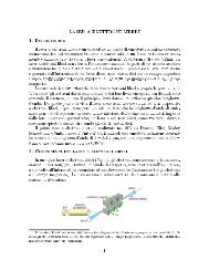
2 Refractive <strong>index</strong> in moving media<br />
Suppose a linear, isotropic, homogeneous medium is moving with a constant<br />
velocity v with respect to an <strong>inertial</strong> laboratory frame of reference K.<br />
A monochromatic electromagnetic wave travelling through it, in <strong>the</strong> <strong>inertial</strong><br />
frame K ′ in which <strong>the</strong> medium is at rest, has, as shown in <strong>the</strong> previous<br />
section, phase velocity u ′ , whose magnitude u ′ is defined by <strong>the</strong> medium<br />
<strong>refractive</strong> <strong>index</strong> n ′ ; which will be its phase velocity magnitude u, or equivalently<br />
<strong>the</strong> medium <strong>refractive</strong> <strong>index</strong> n, measured by an observer at rest with<br />
respect to K?<br />
First of all, <strong>the</strong> <strong>transformation</strong> <strong>laws</strong> <strong>between</strong> K and K ′ are given, in <strong>the</strong><br />
formalism of Special Relativity, by <strong>the</strong> Lorentz boost<br />
⎡<br />
⎡<br />
x 0 γ β x γ β y γ β z γ ⎡<br />
⎢x 1<br />
β<br />
⎥<br />
⎣x 2 ⎦ = x γ 1 + (γ − 1) β2 x<br />
β 2<br />
(γ − 1) β xβ y<br />
β 2<br />
(γ − 1) β xβ z<br />
x ′0<br />
β 2<br />
⎢β y γ (γ − 1) β yβ x<br />
β 2<br />
1 + (γ − 1) β2 y<br />
β 2<br />
(γ − 1) β yβ z<br />
⎢x ′1<br />
⎥<br />
⎥ ⎣x ′2 ⎦ (3)<br />
β 2 ⎦<br />
x 3 ⎤<br />
where<br />
⎣<br />
β z γ<br />
(γ − 1) β zβ x<br />
β 2<br />
(γ − 1) β zβ y<br />
β 2<br />
x µ = (ct, x, y, z)<br />
β = (β x , β y , β z ) = v c<br />
γ = ( 1 − β 2) − 1 2<br />
1 + (γ − 1) β2 z<br />
β 2<br />
⎤<br />
x ′3 ⎤<br />
3
Equation (3) can also be written as<br />
x 0 = γ(x ′0 + β · x ′ )<br />
(4a)<br />
x = x ′ + γx ′0 β + γ − 1<br />
β 2 ( β · x ′ ) β (4b)<br />
which will come handy during calculations; <strong>transformation</strong>s (3) and (4) are<br />
valid for any contravariant four-vector<br />
a µ = (a 0 , a)<br />
when substituting it to x µ in <strong>the</strong> formulas.<br />
Now let’s consider <strong>the</strong> wave phase in K ′<br />
ψ ′ := ω ′ t ′ − k ′ · x ′<br />
where ω ′ is <strong>the</strong> wave frequency and k ′ is its wave vector; we postulate 2 this<br />
quantity is a Lorentz scalar, that is, invariant with respect to any Lorentz<br />
<strong>transformation</strong>, in particular <strong>the</strong> one beetween K and K ′ :<br />
ψ = ψ ′<br />
If we define <strong>the</strong> 4-tuple<br />
it’s easy to see that<br />
( ω<br />
)<br />
k µ =<br />
c , k<br />
ψ = k µ x µ<br />
and that for it to satisfy <strong>the</strong> Lorentz scalar condition for any choice of x µ , k µ has<br />
to be a four-vector. Remembering that<br />
|k ′ | = |ω′ |<br />
c n′ ⇒ k ′ = |ω′ |<br />
c n′ ˆk ′<br />
and applying <strong>transformation</strong> (4a), we get<br />
ω = γ(ω ′ + n ′ |ω ′ | β · ˆk ′ ) (5)<br />
which describes Doppler effect. If k µ is a four-vector, <strong>the</strong> scalar product<br />
k µ k µ = ω2<br />
c 2 − ω2<br />
c 2 n2<br />
2 Physical motivation for this postulate lies in <strong>the</strong> <strong>transformation</strong> <strong>laws</strong> of E and B; moreover,<br />
as we will see, this hypo<strong>the</strong>sis leads to <strong>the</strong> equation describing Doppler effect, which is<br />
experimentally verified.<br />
4
is a Lorentz scalar, which means<br />
ω 2<br />
c 2 − ω2<br />
c 2 n2 = ω′2<br />
c 2 − ω′2<br />
c 2 n′2<br />
n =<br />
√<br />
⇓<br />
(n ′2 − 1) ω′2<br />
ω 2 + 1<br />
Using equation (5) we finally get <strong>the</strong> <strong>transformation</strong> law for <strong>the</strong> <strong>refractive</strong><br />
<strong>index</strong>:<br />
√<br />
(n ′2 − 1) + γ 2 (1 − ω′<br />
|ω<br />
n =<br />
′ | n′ β · ˆk ′ ) 2<br />
∣<br />
∣γ(1 − ω′<br />
|ω ′ | n′ β · ˆk ′ ) ∣<br />
3 An application: Fresnel drag coefficient<br />
Let’s consider <strong>the</strong> simpler case of a wave travelling in <strong>the</strong> same direction as<br />
<strong>the</strong> medium, coinciding with <strong>the</strong> x-axis direction:<br />
k ′ = (k ′ , 0, 0) β = (β, 0, 0) u ′ = (u ′ , 0, 0)<br />
Moreover, <strong>the</strong> orientation of <strong>the</strong> x-axis we will chosen such that u ′ is positive,<br />
which means<br />
n ′ =<br />
c<br />
|u ′ | = c u ′<br />
Remebering that<br />
k ′ = ω′<br />
<strong>transformation</strong>s (4) for k µ become<br />
u ′<br />
v := βc<br />
ω = γω ′ ( 1 + v u ′ )<br />
(<br />
ω 1<br />
u = γω′ u ′ + v )<br />
c 2<br />
Writing ω ′ in terms of ω in <strong>the</strong> first equation, and substituting it in <strong>the</strong><br />
second one we get<br />
( )<br />
ω 1 +<br />
vu ′<br />
u = ω c 2<br />
u ′ + v<br />
which gives <strong>the</strong> <strong>transformation</strong> law for <strong>the</strong> phase velocity 3<br />
u = u′ + v<br />
1 + vu′<br />
c 2<br />
3 Note it is identical to <strong>the</strong> relativistic velocity addition formula for collinear velocities.<br />
5
In terms of <strong>the</strong> <strong>refractive</strong> <strong>index</strong>, this becomes<br />
( )<br />
u = c 1 +<br />
vn ′<br />
c<br />
n ′ 1 + v<br />
cn ′<br />
which, in <strong>the</strong> first order approximation in β becomes<br />
u ≈ c (<br />
n ′ + v 1 − 1 )<br />
n ′2<br />
(6)<br />
The term<br />
1 − 1<br />
n ′2<br />
is called Fresnel drag coefficient, and equation (6) was experimentally verified<br />
by <strong>the</strong> french physicist Hippolyte Fizeau in 1851, half a century before<br />
Special Relativity was formulated. Equation (6) also includes <strong>the</strong> correction<br />
made by Lorentz in 1895 to <strong>the</strong> original Fresnel formula, to account for <strong>the</strong><br />
effects due to dispersion: in fact, in our derivation<br />
n = n(ω) n ′ = n ′ (ω ′ )<br />
and <strong>the</strong> formulas automatically include Doppler effect, which changes <strong>the</strong><br />
wave frequency <strong>between</strong> <strong>the</strong> two <strong>frames</strong>.<br />
References<br />
[1] J.D. Jackson: Classical Electrodynamics. Wiley, 3rd edition, 1999.<br />
[2] L.D. Landau, E.M. Lifshitz, and L.P. Pitaevskii: Electrodynamics of continuous<br />
media, volume 8 of Course of Theoretical Physics. Pergamon, 2nd edition,<br />
1984.<br />
[3] A. Sommerfeld: Optics, volume 4 of Lectures on Theoretical Physics. Academic<br />
Press, 1954.<br />
[4] C. Wang: Wave four-vector in a moving medium and <strong>the</strong> Lorentz covariance of<br />
Minkowski’s photon and electromagnetic momentums. ArXiv e-prints, 2011.<br />
6