An Analytical Delay Model for RLC Interconnects - UCSD VLSI CAD ...

Submitted to IEEE Trans. on CAD
An Analytical Delay Model for RLC Interconnects
Andrew B. Kahng and Sudhakar Muddu
UCLA Computer Science Department, Los Angeles, CA 90095-1596 USA
abk@cs.ucla.edu, sudhakar@cs.ucla.edu
Abstract
Elmore delay has been widely used to estimate the interconnect delays in the performance-driven
synthesis and layout of VLSI routing topologies. For typical RLC interconnections, Elmore
delay can deviate signicantly (by up to 33% or more) from SPICE-computed delay, since it is
independent of inductance. Here, we develop an analytical delay model based on rst and second
moments to incorporate inductance eects into the delay estimate for interconnection lines. Delay
estimates using our analytical model are within 10% of SPICE-computed delay across a wide range
of interconnect parameter values. We also extend our delay model for estimation of source-sink
delays in arbitrary interconnect trees. Even for the small tree topology considered, we observe
signicant improvement of at least 20% in the accuracy of delay estimates when compared to
the Elmore model, even though our estimates are as easy to compute as Elmore delay. The
speedup of delay estimation via our analytical model is several orders of magnitude compared to
simulation methodology such as SPICE.
1 Introduction
Accurate calculation of propagation delay in VLSI interconnects is critical to the design of high
speed systems. With the evolution of VLSI technology, transmission line eects now play an
important role in determining interconnect delays and system performance. Various techniques
have been proposed for the delay analysis of interconnects. These techniques are based on either
simulation techniques or (closed-form) analytical formulas. Simulation tools such as SPICE give
the most accurate insight into arbitrary interconnect structures, but are computationally expensive.
Transient simulation of lossy interconnects based on convolution techniques is presented in
[8, 13]. Faster techniques based on moment computations are proposed in [11, 12,17,19]. Since
these methods are too expensive to be used during iterative layout optimization, the Elmore delay
[2] approximation (which represents the rst moment of the transfer function) is the most widely
This work was supported by NSF grant MIP-9257982.
1

*** DO NOT PROPAGATE this draft or information contained within ***
used delay model in the performance-driven design of clock distribution and Steiner global routing
topologies. However, Elmore delay cannot accurately estimate the delay for RLC interconnect
lines, i.e., the representation for interconnects whose inductive impedance 1 cannot be neglected
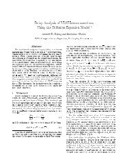
[4]. To see the eect of inductance impedance on the response, consider a 2-port model for an
interconnect driven by a step input with nite source impedance. Figure 1 compares the RC and
RLC line responses computed by SPICE3e: 90% threshold delay is288ps for the RLC model,
but is 358 ps for the RC model. Elmore delay, which does not depend on line inductance, will
yield the same delay estimate of 386 ps for both the RC and the RLC cases. More generally, the
Elmore delay formula gives good estimates if the interconnect lines are RC or overdamped, but
gives overestimates for RLC or underdamped interconnects. This inaccuracy can be harmful for
current performance-driven routing methods which try to optimize interconnect segment lengths
and widths (as well as drivers and buers).
RLC Model
RC Model
Figure 1: Comparison of SPICE3e responses at the end of an interconnect line driven by a
step input and terminated with a capacitive load using both RC and RLC 2-port models.
The 90% threshold delay for the RLC modelis288ps, and for the RC model the delay is
358 ps. The driver resistance is 10:0 and the load capacitance at the end of the line is 2:0
pF . The interconnect line parameters are R =0:075 =m, L =0:123 pH=m, C =8:8
fF=m; the length of the line is 400 m.
This paper gives a new and accurate analytical delay estimate for distributed RLC interconnects
which considers the eect of inductance. Previous moment-based approaches (e.g.,
1 Inductive impedance is 2fL, wheref is the frequency of operation.
2

*** DO NOT PROPAGATE this draft or information contained within ***
[9, 11,8]) can compute a delay estimate only from a simulated response but not from an analytical
formula. To experimentally validate our analysis and delay formula, we model VLSI
interconnect lines having various combinations of source and load parameters, and obtain delay
estimates from SPICE, Elmore delay and the proposed analytical delay model. The delay estimate
using SPICE is extracted from a computed response at the desired node, whereas the other
two models are analytical (closed-form) expressions. Over our range of test cases, Elmore delay
estimates can be as much as 50% from the SPICE-computed delays, while our analytical delay
model estimates are within 15% of SPICE delays. We also extend our delay model to estimate
source-sink delays in arbitrary interconnect trees. For the small tree topology considered, delay
estimates using our analytical model are within 15% of SPICE-computed delays. While Elmore
delay estimates vary by asmuch as 35% from the SPICE-computed delays. Since our analytical
model has the same time complexity as the Elmore model, we believe that it can be useful in
present-day performance-driven routing methodologies.
The organization of our paper is as follows. In Section 2 we discuss previous analytical delay
models for distributed interconnect lines. Section 3 presents a new analytical delay model model
for a distributed RLC line, and nally Section 4 extends our delay model for interconnection
trees.
2 Previous Analytic Delay Models
The transfer function of an RLC interconnect line with source and load impedance (Figure 2)
can be obtained using the ABCD parameters [1] as
H(s) = V 2(s)
V 0 (s) = 1
h i cosh(h)+
Z S
Z 0
sinh(h) + 1
Z T
where = p (r + sl)sc is the propagation constant andZ 0 =
impedance; r = R h ;l = L h ;c = C h
[Z 0 sinh(h)+Z S cosh(h)]
q
R+sL
sC
(1)
is the characteristic
are resistance, inductance, and capacitance per unit length
and h is the length of the line. To compute the RLC line response from the transfer function, the
method of Pade approximation has been used by, e.g., [9, 10]. The output transfer function is
expanded into a Maclaurin series of s around s = 0, and the series is truncated to desired order. 2
2 The work of [8] used a recursive convolution based approach and expanded the admittance and the propagation
coecient term around s = 1.
3

*** DO NOT PROPAGATE this draft or information contained within ***
In general, analytical computation of the exact voltage response is very tedious and is usually in
the form of an innite series.
ZS
Distributed RLC line
v (t) i (t)
v (t) i (t)
0 0 1 1
i (t) v (t)
2 2
Z T
Figure 2: 2-port model of a distributed RLC line with source impedance Z S
impedance Z T .
and load
Ecient delay estimates for RC lines are typically derived by considering a single interconnect
line with resistive source and capacitive load impedances; delay formulas for an interconnect tree
entail recursive application of the formula for a single line. The analytical Elmore delay [2]
estimate, Sakurai's heuristical delay formula [15, 16] and single pole delay estimates of [3] have
been widely used.
Elmore delay is dened to be the rst moment of the system impulse response, i.e., the
coecient ofs or the rst moment in the system transfer function H(s). Applying this
denition to H(s) in Equation (1) and considering a source resistance R S and a capacitive
load C T , the Elmore delay for a distributed RC or RLC line model is
T ED = R S (C + C T )+R( C 2 + C T ) (2)
By considering only one pole in the transfer function, i.e, approximating the denominator
polynomial to only rst moment, the single pole response can be obtained as in [3]. The
single pole of the transfer function is equal to the inverse of the Elmore delay T ED . Hence,
the delay at arbitrary thresholds of the single pole response can be directly related to Elmore
delay (Elmore delay actually corresponds to the 63:2% threshold voltage of the single pole
response). For example, delay at 90% threshold voltage is
T 0:9 = 2:3 T ED =1:15RC +2:3(R S (C + C T )+RC T ) (3)
Sakurai [15] alsogave response and delay calculations for the distributed RC line. He calculates
the time-domain response from the transfer function using the Heaviside expansion
4

*** DO NOT PROPAGATE this draft or information contained within ***
over poles of the transfer function. Then, he approximates the response using a single pole
and observes the variation of delay with respect to source and load parameters; a 90%
threshold delay estimate is heuristically obtained as
T 0:9 (h) =1:02RC +2:3(R S (C + C T )+RC T )
Note that Sakurai's heuristic delay formula is almost identical to the Elmore delay equation (3).
In this paper, to compute the 90% threshold delay according to the Elmore model we apply
Equation (3). Since these single pole delay estimates cannot accurately estimate delay for RLC
interconnects, Zhou et al. [19] proposedatwo-pole approximation for the transfer function to
compute the response at the load for RLC interconnection trees. However, this technique is
based on response computation and does not provide any analytical expression for delay; it is too
time-consuming to be used in iterative optimization of layout. Recently, [7] proposed to improve
the Elmore delay model by using higher-order moments; this work gave a heuristic net delay
model equal to the sum of the rst moment (M 1 ) and its standard deviation. 3
3 A New Analytical Delay Model
We nowdevelop a simple closed-form delay estimate, based on rst and second moments, which
considers the eect of inductance.
To our knowledge, this is the rst analytical delay model
which handles arbitrary threshold voltages and inductance eects for a distributed line. We give
experimental conrmation via 90% threshold delay estimates 4 which we compare against SPICE
output. 5
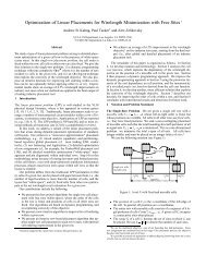
We model an arbitrary interconnect line as follows: (i) the source is modeled as a resistive
and inductive impedance (Z S = R S + sL s ), and (ii) the load at the end of the interconnect line
is modeled using capacitive impedance. Thus, the transfer function for the interconnect line of
p 3 Standard deviation is equal to = jM1 2 , M2j. In the early drafts of our paper [6] we also considered exactly
the same model; however, it turns out that this model is not accurate for various source and load parameters, as
discussed in detail by [6]. The full version of our paper [6] studies various combinations of rst and second moments,
of which the analytical model described here performs best.
4 Our analytical model extends to any threshold delays; we simply give the derivation for 90% delay threshold.
5 SPICE simulation results are obtained using SPICE3 and the built-in LTRA (lossy transmission line) model,
which is based on convolution techniques [13].
5

*** DO NOT PROPAGATE this draft or information contained within ***
S
R
S
L
S
A B T
Distributed RLC line
v (t) i (t) v (t) i (t)
0 0 1 1
i (t)
2 v 2
(t)
C T
Figure 3: 2-port model of a distributed RLC line with resistive and inductive source
impedance, and capacitive load impedance.
Figure 3 is
H(s) =
where Z T = 1
sC T
, Z S = R S + sL S , Z 0 =
cosh(h) 1+ Z S
Z T
+ sinh(h)
ZS
Z 0
+ Z 0
q
R+sL
sC
1
Z T
and h = p (R + sL)sC. We truncate this
transfer function by expanding the hyperbolic functions around s = 0; expansion around s = 1
is not necessary since we consider only the rst few coecients of the transfer function. I.e.,
expanding cosh and sinh as innite series and collecting terms up to the coecient ofs 2 in the
denominator, we obtain the truncated transfer function
H(s)
1
1+sb 1 + s 2 b 2
with coecients
b 1 = R S C + R I C T + RC 2 + RC T
b 2 = R SRC 2
6
+ R SRCC T
2
+ (RC)2
24
+ R2 CC T
6
+ L S C + L S C T + LC 2 + LC T (4)
Note that the rst and second moments of the transfer function can be obtained from the coef-
cients b 1 and b 2 , i.e., M 1 = b 1 and M 2 = b 2 , b 1 2.We use the coecient notation b 1 ;b 2 and the
moment notation M 1 ;M 2 interchangeably according to the simplicity of the expression. Depending
on the sign of b 2 , 4b 1 2, the poles of the transfer function can be either real or complex. We
separately derive our delay model from the two-pole response for each of these cases.
Real Poles:
The two-pole methodology [6, 19] yields the following response for the case of real poles:
v(t) =V 0 (1 , s 2
s 2 , s 1
e s 1t + s 1
s 2 , s 1
e s 2t )
6

*** DO NOT PROPAGATE this draft or information contained within ***
Source Load Delay from Analytical Delay
Response Models
R S L S C T SPICE Elmore New Model
pH pF ps ps ps
50 2.46 0.176 22.33 22.93 22.21
100 2.46 0.176 45.30 45.20 45.70
500 2.46 0.176 224.50 223.50 228.95
1000 2.46 0.176 446.20 446.4 457.46
25 2.46 1.76 107.10 108.40 108.65
50 2.46 1.76 210.10 210.80 214.74
100 2.46 1.76 415.20 415.40 425.10
500 2.46 1.76 2052.60 2053.0 2103.68
1000 2.46 1.76 4099.50 4100.0 4101.30
Table 1: 90% threshold voltage delay estimates for combinations of source and load parameters
for which the poles of the response are real (i.e., overdamped response). The interconnect
line parameters are R =0:015 =m, L =0:246 pH=m and C =0:176 fF=m and the
length of the interconnect is 100 m.
where
s 1;2 =
,M 1
2
q
4M 2 , 3M 2 1
q
= ,b 1 b 2 , 4b 1 2
2b 2
The condition for the poles to be real is (4M 2 , 3M 2 1
)=(b 2 1
, 4b 2 ) 0. Since s 2 , s 1 = ,
is negative, the coecients
s 2
s 2 ,s 1
and s 1
s 2 ,s 1
p
b 2 1 ,4b 2
b 2
are positive. Also, since the magnitude js 2 j is greater
than js 1 j, the second term in the time-domain response decreases rapidly compared to the rst
term. Hence, the two-pole response can be approximated (lower-bounded) as
v(t) V 0 (1 , s 2
s 2 , s 1
e s 1t )
Since the voltage is lower-bounded, the delay obtained is an upper bound on the actual delay. The
delay r (the subscript indicates the case of real poles) at threshold voltage v th can be obtained
via
Letting K r =ln
(s2 , s 1 )(1 , v th )
s 1 r =ln
s 2
1
[1 + p
b 1
2(1,v th )
b 2 1 ,4b 2
r = K r
js 1 j = K M 1 +
r
] ,wehave
0
= , ln @
1
2(1 , v th ) [1 + b
q
1
]
b 2 , 4b 1 2
q
4M 2 , 3M 2 1
2
q
2b 2
= K r
b 1 , b 2 , 4b 1 2
1
A
7

*** DO NOT PROPAGATE this draft or information contained within ***
i.e., K r is a function of the coecients b 1 and b 2 . For the wide range of source, load and
interconnect parameter values considered in our simulations (see Table 1), we nd that K r
actually almost a constant: the plot on the left side of Figure 4 shows the linear regression used
to nd the value K r =2:36 which givesavery strong t between SPICE delay values and 1
js 1 j .
The variation of K r with the quantity X = b 2
b 2 1
r =2:36
b 1 ,
2b
q 2
b 2 , 4b 1 2
is further discussed in [6]. Thus, we use
=2:36 (M 1 +
q
4M 2 , 3M 2)
1
; (5)
2
the resulting delay estimates are compared against those of various other methods in Table 1.
We see that our analytical delay model gives estimates close to those obtained from SPICE, but
as expected Elmore delay also gives good estimates for this case where the interconnect response
is overdamped.
is
500
10
450
9
400
8
SPICE Delay (ps)
350
300
250
200
150
SPICE Delay (ps)
7
6
5
4
3
100
2
50
0
0 20 40 60 80 100 120 140 160 180 200
1/s1
1
0
0 1 2 3 4 5 6
1/β
Figure 4: The plot on the left shows the strong linear t between SPICE delay and 1
js 1 j
for
real poles with K r =2:36. The plot on the right shows the strong linear t between SPICE
delay and 1 for complex poles with K c =1:66.
Complex Poles
The condition for complex poles is (4M 2 , 3M 2 1 )=(b2 1 , 4b 2) 0. The time-domain response
for complex poles is given by
p !
2 +
v(t) =V 0 1 ,
2
e ,t sin(t + )
p
M
where = 1
3M
=
2(M
1 2 1 2 ,4M 2
and = tan ,1 ( ). Using the above equation and threshold
,M 2) 2(M
1 2 ,M 2)
8

*** DO NOT PROPAGATE this draft or information contained within ***
voltage v th ,weget
e ,t sin( t + ) =
1 , v th
q
1+(
)2 (6)
The delay atagiven threshold voltage can be computed by solving for time in Equation (6)
recursively. One way to solve the recursive Equation (6) is to approximate the time variable in
the exponential term by Elmore delay, i.e., substitute T ED for time t. Expanding sine as a Taylor
series and considering only the rst term yields
Therefore,
where K c =
e ,T ED
sin( c + ) e ,T ED
( c + ) =
c = K c
1 , v th
q
1+(
)2
(1,v th )e T ED
, . Substituting for and using M p1+( 1 = b 1 and M 2 = b 2 , b
)2 1 2, our
delay estimate is given by
c = K c
= K 2b 2
c q
4b 2 , b 2 1
Even though K c is function of b 1 and b 2 , for a wide range of interconnect, source, and load
parameters it too is almost a constant. We determined the constant value K c =1:66 again by
nding a good t between SPICE delay values and 1 ,asshown on the right side of Figure 4.
Therefore, the 90% threshold delay estimate for complex poles is
c =1:66 q
2b 2
2(M
=1:66 1
, M 2 )
q
4b 2 , b 2 1
3M 2 , 4M 1 2
: (7)
Table 2 shows delay values for various combinations of source, load and interconnect parameters
assuming the value of K c obtained by this regression analysis. The delay estimates using
our analytical model are within 10% of SPICE-computed delay estimates, while Elmore delay
estimates vary by asmuch as 33% from SPICE-computed delays. Hence, for the case of complex
poles (i.e., underdamped response), the Elmore model is no longer acceptably accurate. Last, we
consider the special case in which poles are equal, i.e., a double pole conguration.
Double Poles
The condition for a double pole is (b 2 1
, 4b 2 ) = 0. The double-pole response is
V (s) = V 0
s
1
1+b 1 s + b 2 s = V 0
2 s
1
b 2 (s , s 1 ) 2 = V 0
9
1
s , 1
s , s 1
, 2 b 1
1
(s , s 1 ) 2

*** DO NOT PROPAGATE this draft or information contained within ***
Source Load Delay from Analytical Delay
Response Models (% error)
R S L S C T SPICE Elmore New Model
pH pF ps ps ps
10 0.0246 0.0176 1.22 0.90 (26%) 1.30 (6%)
15 0.0246 0.0176 1.33 1.31 ( 2%) 1.38 ( 4%)
20 0.0246 0.0176 1.47 1.71 ( 16%) 1.51 ( 3%)
25 0.0246 0.0176 1.60 2.12 ( 33%) 1.64 ( 3%)
10 0.0246 0.176 4.50 5.12 ( 14%) 4.25 ( 6%)
15 0.0246 0.176 5.85 7.32 ( 25%) 5.31 ( 9%)
20 0.0246 0.176 7.90 9.55 (21 %) 8.60 ( 7%)
10 2.46 0.0176 1.31 0.90 ( 31%) 1.40 ( %)
15 2.46 0.0176 1.40 1.31 ( 7%) 1.49 ( 7%)
20 2.46 0.0176 1.55 1.71 ( 10%) 1.59 ( 2%)
25 2.46 0.0176 1.63 2.12 ( 30%) 1.69 ( 4%)
10 2.46 0.176 4.65 5.10 ( 10%) 4.30 ( 8%)
15 2.46 0.176 5.85 7.33 ( 25%) 5.30 ( 9%)
20 2.46 0.176 7.98 9.55 ( 19%) 8.70 ( 9%)
10 24.6 0.0176 1.80 0.90 ( 50%) 1.96 ( 9%)
15 24.6 0.0176 1.89 1.31 ( 31%) 2.06 ( 9%)
20 24.6 0.0176 2.00 1.71 ( 15%) 2.15 ( 7%)
25 24.6 0.0176 2.19 2.11 ( 4%) 2.21 ( 1%)
10 24.6 0.176 5.65 5.10 ( 10%) 5.44 ( 4%)
15 24.6 0.176 6.50 7.33 ( 13%) 5.95 ( 8%)
20 24.6 0.176 7.66 9.55 ( 25%) 6.97 ( 9%)
25 24.6 0.176 9.47 11.78 ( 24%) 9.26 ( 2%)
Table 2: 90% threshold voltage delay estimates for the combinations of source and load parameters
for which the poles of the response are complex (i.e., underdamped congurations).
The interconnect line parameters are R =0:015 =m, L =0:246 pH=m and C =0:176
fF=m and the length of the interconnect is 100 m. The percentage error of each delay
model with respect to SPICE is also given.
where s 1 = , b 1
2b 2
, and the time-domain response is given by v(t) =V 0
1 , e
ts 1
, 2t
b 1
e ts 1
. The
delay at 90% threshold is
0:9 = 2b 2
b 1
which gives a recursive equation for K d , i.e.,
K d =ln
ln 10(1 + 2T
0:9 2b 2 b 1
) = K d = K d
b 1 b 1 2
10(1 + 2T 0:9
b 1
=ln(10(1 + K d ))
10

*** DO NOT PROPAGATE this draft or information contained within ***
from which K d 3:9. Thus, in the case of a double pole the 90% threshold delay is estimated as
0:9 = K d b 1
2 =1:95b 1 (8)
which is independent of the inductance value and dierent from the Elmore delay expression.
I3
N4
I2
N3
I4
N5
I6
N7
N1
I1
N2
I5
N6
I7
N8
I8
N9
Figure 5: A simple interconnection tree consisting of distributed RLC lines. The lengths
of the various interconnects are given in Table 3.
4 Interconnection Trees
Finally, wenow describe the extension of our analytical model to estimate delays in arbitrary
interconnect trees. An RLC network is called an RLC tree if it does not contain a closed path
of resistors and inductors, i.e., all resistors and inductors are oating with respect to ground and
all capacitors are connected to ground. Consider an RLC interconnect tree with root (or source)
S and set of sinks (or leafs) L = fL 1 ;L 2 ;:::;L n g. The unique path from root S to the sink node
i is denoted by p(i) and is referred as the main path. The edges/nodes not on the main path are
referred as the o-path edges/nodes. We model each edge on the main path of the tree using a
lumped RLC segment, e.g., an L, T, or model. We replace the o-path subtree rooted at node
k with the total subtree capacitance at node k. (Figure 6 shows an example of a main path where
each branch in the tree is replaced by RLC segments, and the o-path subtrees are replaced by
their respective subtree capacitances.) Hence, at any nodek the total capacitance is given by
11

*** DO NOT PROPAGATE this draft or information contained within ***
Interconnect
Length
m
I1 50
I2 100
I3 50
I4 200
I5 100
I6 50
I7 100
I8 200
Table 3: The length of various interconnects in the tree of Figure 5.
C 0 k
= C k if no o-path subtree at node k
= C k + C T (k) if node K has o-path subtree T (k)
where C k is the capacitance at the node and C T (k) is the o-path subtree capacitance at node
k. The k th coecient b k of the transfer function for the general RLC circuit of Figure 6 can be
expressed using the following recursive equation [5]:
b N +1
k
= R N
N X
j=1
C 0 j b j k,1 + L N
NX
j=1
C 0 j b j k,2 + bN k (9)
where b N K refers to the coecient ofsk in the transfer function between node k and node 1. Note
that b j 0 =1,bj ,1 =0forallj and b1 k
= 0 for all k. Using the above recursive equation the
expressions for the rst and second coecients of the transfer function can be derived as
b N +1
1
= R N
N X
j=1
C 0 j + b N 1
=
b N +1
2
= R N
N X
j=1
C 0 jb j 1 + L N
=
NX
NX
X
NX
i=1
NX
j=1
X
j,1 j,1
C 0 j
R l C 0 j
j=2 l=j i=1 d=i
R i
iX
j=1
C 0 j + b N 2
R d +
C 0 j
NX
NX
C 0 j
j=1 l=j
L l (10)
For any given source and sink pair the coecients b 1 and b 2 can be computed in linear time
by traversing the main path and using the above recursive equation. Using the analytical delay
model developed in the previous section, we can obtain a analytical delay estimate for RLC
12

*** DO NOT PROPAGATE this draft or information contained within ***
R S
V R L V R L
V V R L
N+1
N N N N-1 N-1 N-1
2 1 1
S
C’ C’ C’
V
1
T
N N-1
1
C T
Figure 6: Representation of the main path in the tree, where each distributed line is modeled
using RLC segments.
interconnect trees using the rst and second coecients. Thus, the 90% threshold delay ata
given sink i, depending on the value of (4M 2 , 3M 2 1
), is
p
= K r (M 1+ 4M 2 ,3M1 2 )
for Real poles
2
2(M
T ND (i)
1
= K c
2 ,M 2)
for Complex poles
p
3M 2 1 ,4M 2
= K d M 1
2
for Double poles
(11)
where the rst and second moments are expressed as M 1 = b 1 and M 2 = b 2 , b 1 2. The coecients
of the transfer function are obtained from Equation (10). By contrast, the Elmore delay at
the sink is equal to the rst moment, or the rst coecient b 1 of the transfer function of the
source-sink main path [14]. The 90% threshold delay using the rst moment is simply
T ED (i) =2:3 M 1 (12)
which we emphasize can be inaccurate despite its wide use, since it ignores inductance of the
interconnect line.
We evaluate the eect of our analytical model by considering a simple interconnection tree
shown in Figure 5. We consider the sink node N4 for delay estimation. Each edge on the main
path between the root and node N4 is replaced by atwo L segment model. 6
We then apply
the above described recursive coecient (or moment) computation for the resultant RLC circuit
of the main path. The 90% threshold delays according to both the Elmore model and our new
analytical model are computed using Equations (11) and (12). We also compute the delay at
the given sink node using SPICE3e, where each edge of the tree is modeled using the LTRA
6 Our model is not limited to traditional segment models, and indeed we believe the accuracy of our results
would improve ifwe use non-uniform segment models [5, 18] designed to perfectly match the low-order moments
of the distributed RLC line.
13

*** DO NOT PROPAGATE this draft or information contained within ***
Interconnect Driver Load SPICE Elmore New Model
parameters res. cap. Delay Delay Delay
/m pF ps ps ps
R =0:015
C =0:176 fF 10 0.02 5.7 6.6 5.0
L =0:246 pH
R =0:0015
C =0:176 fF 10 0.2 37 26 31
L =2:46 pH
R =0:015
C =0:176 fF 10 0.2 39 29 32
L =2:46 pH
R =0:0015
C =0:176 fF 10 2.0 179 238 205
L =2:46 pH
R =0:0015
C =0:176 fF 10 2.0 231 238 232
L =0:246 pH
R =0:015
C =0:176 fF 10 2.0 199 270 230
L =2:46 pH
R =0:015
C =0:176 fF 100 2.0 2419 2361 2367
L =2:46 pH
Table 4: 90% threshold delay values for a wide range of interconnect parameters at Node
4 of the tree in Figure 5. We compare SPICE LTRA, and the Elmore model, against our
analytical delay model.
(Lossy Transmission Line) model (with SPICE, we rst compute the response at the sink node
and then obtain the delay for 90% threshold voltage). Table 4 presents delay estimates for a
range of interconnect parameters, driver resistance values, and sink load capacitance values. The
Elmore delay varies by asmuch as 35% from the SPICE-computed delay. However, our new
model is within 15% of the SPICE delay for all examples. Another advantages of our model
is due to simulation complexity.
Our delay estimates also require three orders of magnitude
less computation than SPICE, since they have the same time complexity as the Elmore delay
estimate.
14

*** DO NOT PROPAGATE this draft or information contained within ***
5 Conclusions
Fast delay estimation methods, as opposed to simulation techniques, are needed for incremental
performance-driven layout synthesis. Elmore delay based estimation methods, although ecient,
cannot accurately estimate the delay forRLC interconnect lines. We have obtained an analytical
delay model, based on rst and second moments of RLC interconnection lines, which considers
the eect of inductance. Resulting delay estimates are signicantly more accurate than Elmore
delay. We also extend our delay model to estimate source-sink delays in arbitrary interconnect
trees. Even for the small tree topology considered, we observe signicant improvement ofatleast
20% in the accuracy of our delay estimates, compared to the Elmore model. Since our model has
the same time complexity as the Elmore model, we believe it can be valuable in modern iterative
layout synthesis methodologies. Our ongoing work applies our analytical model to delay-driven
routing tree construction, zero-skew routing, and delay estimation in nets spanning multiple
routing layers (i.e., with modeling of vias).
15

References
[1] L. N. Dworsky, Modern Transmission Line Theory and Applications, Wiley, 1979.
[2] W. C. Elmore, \The Transient Response of Damped Linear Networks with Particular Regard to
Wideband Ampliers", Journal of Applied Physics 19, Jan. 1948, pp. 55-63.
[3] M. A. Horowitz, \Timing Models for MOS Circuits", PhD Thesis, Stanford University, Jan. 1984.
[4] C. C. Huang and L. L. Wu, \Signal Degradation Through Module Pins in VLSI Packaging", IBM
J. Res. and Dev. 31(4), July 1987, pp. 489-498.
[5] A. B. Kahng and S. Muddu, \Two-pole Analysis of Interconnection Trees", Proc. IEEE MCMC
Conf., January 1995, pp. 105-110.
[6] A. B. Kahng and S. Muddu, \Accurate Analytical Delay Models for VLSI Interconnections", UCLA
CS Dept. TR-950034, Sep. 1995.
[7] B. Krauter, R. Gupta, J. Willis, and L. T. Pileggi, \Transmission Line Synthesis", Proc. 32th
ACM/IEEE Design Automation Conf., June 1995, pp. 358-363.
[8] S. Lin and E. S. Kuh, \Transient Simulation of Lossy Interconnect", Proc. 29th ACM/IEEE Design
Automation Conf., June 1992, pp. 81-86.
[9] S. P. McCormick and J. Allen, \ Waveform Moment Methods for Improved Interconnection Analysis",
Proc. 27th ACM/IEEE Design Automation Conf., June 1990, pp. 406-412.
[10] L. T. Pillage and R. A. Rohrer, \Asymptotic Waveform Evaluation for Timing Analysis", IEEE
Trans. on CAD 9, Apr. 1990, pp.352-366.
[11] V. Raghavan, J. E. Bracken and R. A. Rohrer, \AWESpice: A General Tool for the Accurate and
Ecient Simulation of Interconnect Problems", Proc. 29th ACM/IEEE Design Automation Conf.,
June 1992, pp. 87-92.
[12] C. L. Ratzla, N. Gopal, and L. T. Pillage, \RICE: Rapid Interconnect Circuit Evaluator", Proc.
28th ACM/IEEE Design Automation Conf., June 1991, pp. 555-560.
[13] J. S. Roychowdhury and D. O. Pederson, \Ecient Transient Simulation of Lossy Interconnect",
Proc. 28th ACM/IEEE Design Automation Conf., June 1991, pp. 740-745.
[14] J. Rubinstein, P. Peneld and M. A. Horowitz, \Signal Delay inRCTree Networks", IEEE Trans.
on CAD 2(3), July 1983, pp. 202-211.
[15] T. Sakurai, \Approximation of Wiring Delay in MOSFET LSI", IEEE Journal of Solid-State Circuits,
Aug. 1983, Vol.18, No.4, pp. 418-426.
[16] T. Sakurai, \Closed-Form Expressions for Interconnection Delay, Coupling, and Crosstalk in
VLSI's", IEEE Trans. on Electron Devices 40, Jan. 1993, pp. 118-124.
[17] M. Sriram and S. M. Kang, \Fast Approximation of The Transient Response of Lossy Transmission
Line Trees", Proc. ACM/IEEE Design Automation Conf., June 1993, pp. 691-696.
[18] Q. Yu and E. S. Kuh, \Exact Moment Matching Model of Transmission Lines and Application to
Interconnect Delay Estimation", IEEE Trans. VLSI Systems 3, June 1995, pp. 311-322.
[19] D. Zhou, S. Su, F. Tsui, D. S. Gao and J. S. Cong, \A Simplied Synthesis of Transmission Lines
with A Tree Structure", Intl. Journal of Analog Integrated Circuits and Signal Processing 5, Jan.
1994, pp. 19-30.