Munsell Colors in GSA Document.pdf

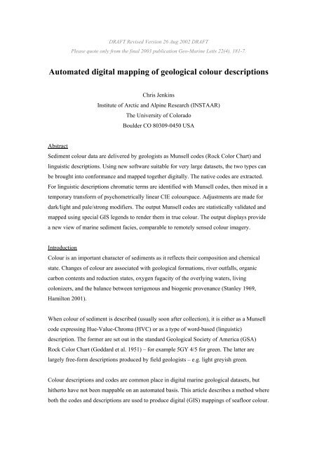
DRAFT Revised Version 26 Aug 2002 DRAFT
Please quote only from the final 2003 publication Geo-Marine Letts 22(4), 181-7.
Automated digital mapping of geological colour descriptions
Chris Jenkins
Institute of Arctic and Alpine Research (INSTAAR)
The University of Colorado
Boulder CO 80309-0450 USA
Abstract
Sediment colour data are delivered by geologists as Munsell codes (Rock Color Chart) and
linguistic descriptions. Using new software suitable for very large datasets, the two types can
be brought into conformance and mapped together digitally. The native codes are extracted.
For linguistic descriptions chromatic terms are identified with Munsell codes, then mixed in a
temporary transform of psychometrically linear CIE colourspace. Adjustments are made for
dark/light and pale/strong modifiers. The output Munsell codes are statistically validated and
mapped using special GIS legends to render them in true colour. The output displays provide
a new view of marine sediment facies, comparable to remotely sensed colour imagery.
Introduction
Colour is an important character of sediments as it reflects their composition and chemical
state. Changes of colour are associated with geological formations, river outfalls, organic
carbon contents and reduction states, oxygen fugacity of the overlying waters, living
colonizers, and the balance between terrigenous and biogenic provenance (Stanley 1969,
Hamilton 2001).
When colour of sediment is described (usually soon after collection), it is either as a Munsell
code expressing Hue-Value-Chroma (HVC) or as a type of word-based (linguistic)
description. The former are set out in the standard Geological Society of America (GSA)
Rock Color Chart (Goddard et al. 1951) – for example 5GY 4/5 for green. The latter are
largely free-form descriptions produced by field geologists – e.g. light greyish green.
Colour descriptions and codes are common place in digital marine geological datasets, but
hitherto have not been mappable on an automated basis. This article describes a method where
both the codes and descriptions are used to produce digital (GIS) mappings of seafloor colour.

The work is part of the dbSEABED programme for the processing of large marine geological
datasets (Jenkins 1997). This style of information processing aims to mine diverse forms of
data and produce a conformable information-rich product which is useful in digital mapping,
statistics, input for models and for queries.
Procedure
Munsell codes
AH Munsell (1923) formalized a colour space which conveys the common perception of
colours through Hue, Value and Chroma. Hue is the spectral content (red, yellow, green, blue,
purple), Value refers to lightness, and Chroma is the vividness or saturation. Schemes using
HVC tend to conform to cultural colour vocabularies (see Roget 1852). A later Renotation
Munsell colourspace (Newhall et al. 1943) corrected some of the distortions of Munsell's
system. This modern Munsell system is very widely used for industrial production and was
formalized in geological sciences by the GSA Rock Color Chart which displays Munsell
codes with their verbal descriptive equivalents and sample colour tablets. The 3 dimensional
Munsell colourspace is visualized as a cylinder, with Hues arranged around the radius (colour
wheel), Chroma radiating away from the axis, and Values increasing axially from base to top.
Since the publication of the Rock Color Chart it has been commonplace to include Munsell
codes among observations during marine geological research. For the colours to be mapped
digitally, the codes have first to be extracted from digital renditions of the various expedition
datasets and manipulated into one common format. For example, 5GY6/2 and 5-6GY6/2
(both incorrect notation), 5GY 6/2 and 5GY 6/2 to 7.5G 4/5 (both correct) are common
variants. In datasets containing over 10 4 attributed sites and where new large datasets are
constantly being added (Jenkins 1997), this task has to be automated. For this project, the
software attempts to parse the internal Munsell code format and reports faulty codes to a
diagnostics file which is used for subsequent corrections. Several software error-traps are also
set against out-of-range inputs and outputs.
The verified and processed Munsell codes are output by the dbSEABED software, alongside
other attributes of the sediments such as rock presence, grain sizes and sorting, carbonate and
organic carbon contents, physical properties, grain type and feature facies (Jenkins 1997).
This allows investigation of their relationships to colour.

Linguistic descriptions
Word-based descriptions of geological materials are almost always in terms of objects,
modifiers and quantifiers. Objects convey in absolute terms the value of an attribute, whether
grain size, composition or colour. Colour examples are green, greenish, grey and greyish.
Modifiers convey a relative meaning, a modification of the attribute, examples being light,
bright and dusky. Quantifiers convey the dominance of the attribute, for example that a
sediment is mainly, occasionally or probably a certain colour. dbSEABED employs this
division to parse sediment descriptions using a fuzzy set theory formalism and a thesaurus
(see Jenkins 1997). Descriptions of colour are extracted from datasets at fields carrying the
general lithological descriptions (e.g. olive green muddy sand) and from fields dedicated to
colour (olive green). A typical colour description combines several chromatic terms with
modifiers and can be quite complex (see Rock Color Chart). The task for a software parser of
colour descriptions is to deal with all the terms in a description correctly in terms of visual
perception, and then to output a useful and reliable quantitative expression for the colour.
Figure 1. Distortions measured in the Renotation Munsell by Indow and Aoki (1983). The
Munsell colourspace is non-linear and unsuitable as a base for performing calculations.
In order to parse colour descriptions, a model of the psychophysical meanings (see Agoston
1979) of specific terms is required. For the colour objects this is straightforward - we adopt
the Munsell Hue/Value/Chroma indices (and then CIE x,y,Y; from Commission
Internationale de l'Eclairage) for the terms, using the GSA Rock Color Chart. However,

modifiers involve relative adjustments of Chroma and Value from a base colour. To deal
objectively with these two concepts, Chroma and Value offsets for the terms relative to the
base colours were measured using the entries in the Rock Color Chart (Fig. 2). These offsets
were then entered in the parsing thesaurus, later to be used as operators by the dbSEABED
software.
Figure 2. Offsets in Value and Chroma observed for various modifier terms in the Rock Color
Chart (Goddard et al. 1951).
Unfortunately, the Munsell colour system is not suitable for the combining of colour terms,
which is necessary to parse a multi-term description. It is psychometrically non-linear in Hue
and Chroma (Fig. 1; Indow and Aoki 1983, Indow 1988) but it is linear in Value. The
manipulations of Hues and Chroma in a parser can be performed in an alternative colour
space such as CIE (see Agoston 1979). CIE colourspace permits linear arithmetic mixing of
colours. It allows for the possibility that an output colour can be achieved by mixing more
than one combination of colour terms and also deals faithfully with complementary colours
(Agoston 1976). The RGB colourspace is unsuitable; it does not represent all natural colours
and is non-linear.

Figure 3. CIE colourspace which is based on human visual response to the colours of light. The CIE
{x,y} instances of the Hathaway (1971) marine data and Rock Color Chart are plotted, projected down
from their various luminance values.
In detail, the calculation of colour output proceeds as follows.
(i) Colour objects chromatic (with Hue/Chroma) and neutral (Value only) are each assigned a
Munsell code based (a) on the Rock Color Chart and also (b) on calibrations performed by
matching single colour terms with Munsell codes using actual marine sediment datasets.
(ii) The codes’ Hue/Value/Chroma coordinates ([ H , V , C]
) are converted to CIE chromacity
(x,y) and luminance (Y) using a look-up-table of 2379 colours which was empirically derived
by Indow and Aoki (1983).
(iii) Weightings ({li
, mi
, n i}
) to the CIE instances are calculated as follows. Terms with the
suffix 'ish' (e.g. greenish) have an implicit weighting, in this case of 50%. Rear significance is
the usual syntax in colour descriptions and is applied through a simple dominance table
depending on the number of terms. A simple weighted mixing of CIE terms is then performed
with output
{ x , y,
Y}
= { x,
y,
Y }
(v) The output is transferred back to Munsell colourspace - H , V , C ]- at the colour of
[ c c c
three-dimensional {x,y,Y/100} cartesian closest approach in the Indow and Aoki (1983) lookup-table.
(vi) Modifying terms (i.e. very pale, greyish, light, medium, deep and very dark) are given
effect on both the Chroma and Value of the output Munsell code, as shown in Figure 2.
Validation

The reliability of the processing was tested in several ways.
(i) The Rock Color Chart provides linguistic colour descriptions (names) and matching
Munsell codes, so the original and parsed Munsell codes can be compared statistically (Fig.
4). For Hue, Value and Chroma the linear regression R 2 statistics were 0.96, 0.68, 0.48,
which is satisfactory. These R 2 values suggest that colour names are much more disciplined
for Hue than in Value (grey levels) and worst for Chroma. A few colour names performed
badly, for example greyish pink (5R 8/2) which outputs too dark (5R 6/1).
(ii) Sensitivity tests were performed, for example, with and without rear-significance
weighting of description terms, without which R 2 statistics (HVC) were: 0.96, 0.67, 0.43 –
marginally worse than with weighting.
(iii) Some large datasets of field colour descriptions carry both linguistic and Munsell code
colour for each sample. In this case however, it is difficult to use statistical analysis to rate
performance of the parser because field observers tend to adopt a wide range of codes for any
one colour. In the Hathaway (1971) dataset of the east coast of the USA, olive corresponds to
10 Munsell codes: Hue 10YR to 2.5Y, Value 3 to 5 and Chroma 2 to 4; white to 4 codes: Hue
2.5Y to 10Y, Value 5 to 6, Chroma 1 to 4. A better form of validation uses a visual check that
processing outputs conform to the original intentions of the colour descriptions. To do this,
on-screen colour squares of the output Munsell codes are generated using the CMC Munsell
display tool of van Aken (1999) and then compared to the input colour names. The technique
has confirmed that valid output colours are produced.
a)
b)

c)
Figure 4. Testing results for the parser using the GSA Rock Color Chart dataset. a. Hue; b. Value; c.
Chroma. Solid lines are the lines of 1:1 correspondence between input and output; dashed line is a
linear regression between the inputs and outputs.
Display
To strike a balance between proper rendering of the colours and a practical total number of
colour variants, the output codes are rounded to increments of 5 in Hue, 3 in Value and 3 in
Chroma. For example, 2.5Y 4/7 is rounded to 5Y 3/6. On datasets which have been processed
to date, 125 different codes are produced, almost completely in greys, reds, browns, yellows,
and greens (Hues N, R, YR, Y, GY). With rounding this is reduced to 40 output codes, of
which only a few slightly exceed the Macadam limits of naturally occurring colours (Agoston
1979).
Symbol colours in the GIS legends are set to approximate the actual colours of the output in
two ways: (i) by reference to the Rock Color Chart; (ii) using the CMC program (van Aken
1999) which can display on-screen the colour of a Munsell code.
Application

The procedure is now routinely applied over regions of the ocean floor where sufficient data
are available. The example presented here is of the US Atlantic continental margin, for which
many datasets describe the colours of seabed samples in terms of Munsell codes and wordbased
descriptions. The largest of the datasets is the composite set of Hathaway (1971; Poppe
and Polloni 2000) but there are also many new data. The complex colour mapping that results
(Figs. 5) coincides with the earlier mapping of Stanley (1969) in its generalities, but is a
digital mapping where the spatial resolution of the input data is preserved to the final digital
map display. Furthermore, since the data are digital, they can be viewed at scales from local to
regional and in different coordinate frames.
The observed pattern of colour changes are summarized as follows (Figs 5, 6).
a. A great deal of spatial variability is observed, implying significant patchiness for colour.
Colours which dominate in one zone are also encountered in most other geographic
settings. Black, yellow and yellow-brown colours especially, are few and irregularly
scattered. Nonetheless, several zonal patterns of colour dominance are observed.
b. South of a transition between Cape Hatteras (36 o N) and Delaware Bay ( 39 o N), grey
colours dominate in continental shelf sediments between 1m to 100m WD (Fig. 6, near
‘C’; Fig. 5 for locations). To the north of those latitudes, shelf sediments have greater
chroma, usually in brown (Fig. 6, near ‘A’).
c. Inshore sediments, at depths shallower than 50m, are most often grey (grey, olive grey or
brownish grey) in colour (Fig 6). This includes those parts of Georges Bank shallower
than 100m.
d. Sediments of intense green colour (Fig. 6, near ‘B’) are most common on the outer shelf
and upper slope at depths of 70 to 300m.
e. The Gulf of Maine (41 o to 45 o N) is a partly enclosed deep basin in which relatively deep
water (100m) occurs in close proximity to the coastline. The distribution of colours
deviates from patterns over open-shelf areas. The inshore sediments are dark green;
basinal sediments are pale to medium brown.
An interpretation of the causative factors in seabed colour is not the goal of this paper. The
large-scale interpretation of colour variations provided by Stanley (1969) is essentially
unaltered. This includes that colour variations are only weakly and irregularly related to
seabed physiography and sediment grain size. The strongest correlations appear to be to water
depth and mineralogy, (specifically to coloured minerals such as glauconite, dark grains), and
also to dilution of colour by pale-toned carbonate materials. Some highly scattered colours

such as black and yellow may have local causes such as erosion into older stratigraphy,
concentrations of glacial debris, local benthic biologic productivity, or groundwater efflux.
Discussion and conclusions
This paper describes a new procedure which automates the digital mapping of seabed colour
using large observational datasets (i.e. more than 100,000 attributed sites) and produces GIS
displays in realistic colours. The procedure allows rapid updating of geographic coverages as
new data is acquired and allows both coded (Munsell) and linguistic (description) input data
types to be plotted together, both calibrated. It preserves the spatial heterogeneity (patchiness)
of seabed colour which is apparently very great in most areas.
Using the outputs, it is possible to produce digital maps of sediment and rock colour for
marine and continental areas ranging in scale from local to global – wherever suitable input
data exist. These digital products can be visualized and combined with other data types in
novel ways. This opens up new opportunities for investigation of the dependencies between
seafloor colour, sediment provenance, oceanography and biogeochemistry.

Figure 5. Large scale mapping of seabed colour along the US Atlantic continental margin,
USA. CH – Cape Hatteras, DB – Delaware Bay, GoM – Gulf of Maine.

Figure 6. Re-projection of US Atlantic continental margin seafloor colours by latitude and
water depth (logarithmic scale). The visualization is suitable for investigations of relations
between sediment colour and water mass (temperature, oxygen), and wave and current
energy. Legend same as for Fig. 5; for symbols A-C refer to text.
Acknowledgements
My thanks to the GretagMacbeth Inc for making available online the software tool ‘CMC.exe’
for Munsell Code display; also to NGDC for the online Hathaway (1971) digital dataset. The

USGS Coastal and Marine Geology section and Royal Australian Navy kindly assisted with
funding.
References
Agoston GA (1979) Color Theory and its Application in Art and Design. Springer-Verlag,
Berlin, 131pp.
Goddard EN, Trask PD, de Ford RK, Rove ON, Singewald JT and Overbeck RM (1951)
Rock Color Chart. Geol. Soc. America, Colorado.
Hathaway JC (1971) Data File, Continental Margin Program, Atlantic Coast of the United
States, Vol. 2, Samples Collection and Analytical Data. WHOI Reference 71-15. [Data
file.]
Hamilton LJ (2001) Cross-shelf colour zonation in northern Great Barrier Reef lagoon
surficial sediments. Australian Journal of earth Sciences 48: 193-200.
Indow T and Aoki N (1983) Multidimensional mapping of 178 Munsell Colors. Color
Research Application 8: 145-152
Indow T (1988) Multidimensional Studies of Munsell Color Solid. Psychological Review
95(4): 456-470.
Jenkins CJ (1997) Building a national scale offshore soils database from both word-based and
numeric datasets. Sea Technology 38(12): 25-28.
Munsell AH (1923) A Color Notation. Munsell Color Company, Baltimore, MD.
Newhall SM, Nickerson D and Judd DB (1943) Final Report of the OSA subcommittee on the
spacing of the Munsell Colors. Journal of the Optical Society of America 33: 385-418
Nickerson D (1940) History of the Munsell color system and its scientific application. Journal
of the Optical Society of America 30: 69-77.
Poppe, LJ and Polloni CF (2000) USGS east-Coast Sediment Analysis: Procedures, Database,
and Georeferenced Displays. US Geological Survey Open-File Report 00-358. [CD-
ROM].
Roget PM (1852) Thesaurus of English Words and Phrases. [3 rd Edition.] P.Haddock Ltd,
Bridlington, 671pp.
Stanley DJ (1969) Atlantic Continental Shelf and Slope of the United States – Color of
Marine Sediments. US Geological Survey Professional Paper 529D: 1-15.
van Aken H (1999) Munsell Conversion [version 4.01]. GretagMacbeth LLC, New Windsor,
NY. [Program.]