chapter 3 fundamentals of fluvial geomorphology and stream ...

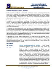
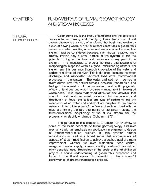
materials. Also, the threshold mobility index is not single valued,but is better characterized by a stochastically determined range ofvalues (Figure 3.2). These findings illustrate that in practice, thegeomorphic threshold behavior of alluvial streams may becomplex.0.1BraidedIncisingMeanderingFigure 3.2 – Probability (%) ofIncising or Braiding as aFunction of SQ 0.5 and D 50 forStreams with Sand Beds --Discharge is Represented byAnnual Flood as First Prioritythen Bankfull (from Bledsoe andWatson 2001)0.010.00190%70%50%30%10%0.1 1D50 (mm)3.2.5 TimeWe all have been exposed to the geologist’s view of time.The Paleozoic Era ended only 248 million years ago, the MesozoicEra ended only 65 million years ago, and so on. Fortunately, wedo not have to concern ourselves with that terminology. Anaquatic biologist may be concerned with the duration of an insectlife stage, only a few hours or days. What we should be aware ofis that the geologist’s temporal perspective is much broader thanthe temporal perspective of the engineer, and the biologist’sperspective may be a narrowly focused time scale. Neitherprofession is good nor bad because of the temporal perspective;just remember the background of people or the literature withwhich you are working.Geomorphologists usually refer to three time scales inworking with rivers: 1) geologic time, 2) modern time, and 3)present time. Geologic time is usually expressed in thousands ormillions of years, and in this time scale only major geologic activitywould be significant. Formation of mountain ranges, changes insea level, and climate change would be significant in this timescale. The modern time scale describes a period of tens of yearsto several hundred years, and has been called the graded timescale (Schumm and Lichty 1965). During this period, a river mayadjust to a balanced condition, adjusting to watershed water andsediment discharge. The present time is considered a shorterperiod, perhaps one year to ten years. No fixed rules govern thesedefinitions. Design of a major project may require less than ten22 Fundamentals of Fluvial Geomorphology and Stream Processes

years, and numerous minor projects are designed and built withinthe limitations of present time (1 to 10 years). Project life oftenextends into graded time. From a geologist’s temporal point ofview, engineers build major projects in an instant of time, basetheir design on data collected during a very brief period, andexpect the projects to last for a significant period in a dynamicallychanging system.In river-related projects, time is the enemy, and time can beour friend and teacher. Recognition of the importance of time isespecially important when considering the post-constructionperformance of a project. Society demands a quick return ofinvestments and the projects are expected to produce positiveresults almost instantaneously. Often, success or failure of aproject is judged within one or two years, regardless of whetherformative events have occurred to drive geomorphic recovery fromconstruction impacts, or design events have occurred to testwhether the project works as it was intended. With respect to themorphological impacts of a river-engineering project, it must beremembered that short-term stream stability or adjustment is notnecessarily indicative of the long-term behavior. For this reason,the morphological performance of stream projects should bemonitored and appraised over a period longer than a few yearsbefore a project is declared to have been successful.3.2.6 ScaleThe size or scale of the fluvial system has a bearing on theway in which it evolves towards a natural equilibrium, adjusts towatershed and climate change, and responds to engineeringinterventions. The time taken for the system to evolve, adjust, orrespond increases with the scale of the system and, as a generalrule, a small stream will react more rapidly to engineering worksthan a large stream. For example, stream adjustments in theMississippi River are still occurring in response to artificialmeander cutoffs constructed in the 1930s, and it may require over100 years before morphological changes triggered by the cutoffsare completed (Biedenharn 1995; Biedenharn and Watson 1997).Conversely, some small bluff line streams in north Mississippi thatwere channelized in the 1960s have adjusted through initialdegradation, secondary aggradation, and dynamic stability within aperiod of less than 25 years (Watson et al. 2002a).The physical size of the stream also conditions and maylimit the type of engineering works that are appropriate andfeasible. While the materials involved in alluvial stream mechanics(basically water, sediment, and vegetation) are scale-independent,the ways that these materials interact are not. For example, themorphological impact and significance of a large tree on the bankof a small stream is quite different to that of a similar tree on theFundamentals of Fluvial Geomorphology and Stream Processes 23

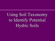
ank of a large river. From an engineering perspective, it isparticularly important to recognize that analyses, techniques, andsolutions designed for one scale of stream may not be directlytransferable to another. Deciding whether an analytical tool,stabilization technique, or stream enhancement solution developedfor streams of a particular size is transferable across streams atother scales demands a thorough understanding of theunderpinning science and engineering principles involved. It is notenough to have demonstrated repeatedly that a given approachworks when applied to streams of a particular scale. Before tools,techniques, or solutions developed in one system scale arepromulgated for wider application, it must be established how andwhy they work. Principles, such as stabilizing a retreating banklineby increasing bank erosion resistance and mass stability orretarding near bank velocities, are transferable across differentscales of river; however, the hydraulic models, bank stabilityanalyses, and structural measures appropriate to control bankretreat successfully may not be scale-independent.3.3 STREAM MORPHOLOGYAlluvial rivers and streams are dynamic and continuouslychange position, shape, and other morphological characteristics inresponse to variations in discharge, sediment load, and boundaryconditions. It is, therefore, important to study, not only the existingmorphology of the river, but also the possible variations during thelifetime of the project. The morphology of the river is determined bythe water discharge, quantity and character of the sediment load,characteristics of the bed and bank materials (including vegetationeffects), geologic controls, and valley topography. Morphologicalchanges and adjustments take place in response to variations inany of these parameters through time or human activities. Topredict the behavior of a river in a natural state or as affected byhuman activities, we must understand how fluvial and geotechnicalprocesses operate on the boundary materials to form and adjustthe morphological features of the stream through time.A schematic diagram defining the morphological featuresassociated with straight and meandering streams is shown inFigure 3.3. The thalweg is the trace of the deepest point of thestream. The thalweg and associated line of maximum velocitycross from side to side within the stream, and this pattern of flowaffects the overall cross-sectional geometry of the stream. At abend, there is a concentration of flow in the outer half of the streamdue to secondary flow. This causes the scour depth to increase atthe outside of the bend, to produce a pool. As the thalwegcrosses the stream downstream of a bend, the velocity distributionand cross-sectional shape become more symmetrical and scour24 Fundamentals of Fluvial Geomorphology and Stream Processes

depths decrease due to deposition of sediment eroded from thepool upstream. This area is known as the riffle or crossing.Figure 3.3 – FeaturesAssociated with Straight andSinuous Rivers (FederalInteragency Stream RestorationWorking Group (FISRWG)1998)Pool-riffle sequences are characteristic of cobble, gravel,and mixed load rivers of moderate gradient (S < 5%) (Sear 1996).Riffles are topographic high points in an undulating bed profile andpools are low points. Typically, sediment grain size is coarser onriffles than in pools. A sorting mechanism was proposed by Keller(1971) to explain this variation. According to Keller (1971), finesediment is removed from riffles during low flows and deposited inpools because velocities and bed shear stresses are higher atriffles. As discharge rises, velocity and shear stress in the poolincrease quickly, with little, if any increase over the riffle.Consequently at the formative flow, velocities and shear stressesin pools are higher than that at riffles, resulting in scour of largesediment from the pools and deposition on the next riffledownstream. However, field evidence for this conceptualexplanation is equivocal. Ashworth (1987), Petit (1987), andClifford (1990) have measured the shear stress reversalhypothesized by Keller, but other studies have suggested that pooland riffle velocities equalize at bankfull flow, but do not reverse(Lisle 1979; Carling 1991).Yalin (1971) suggests that pools and riffles may beexplained by macro-turbulent eddies generated at the boundariesof a straight, uniform stream that produce alternate accelerationand deceleration of flow. Yalin showed theoretically that thelongitudinal spacing of faster and slower zones would average πw(w = stream width) for macro-turbulent eddies with diameterssimilar to the stream width. This is about half the riffle spacing of 5to 7 times the stream width observed in nature (Keller and Melhorn1973). Hey (1976) proposed a resolution to this differencebetween theory and observation by proposing that the largestFundamentals of Fluvial Geomorphology and Stream Processes 25

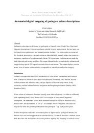
eddies in a stream do not scale on the width, but the half-width,with the centerline of the stream acting as a line of symmetry.According to Hey’s hypothesis, riffles would be spaced at 2πw,which better accords with observations.The cross-sectional shape of a stream varies systematicallywith distance along the stream in relation to the plan geometry, thetype of stream, and the characteristics of the sediment forming andtransported within the stream. The cross section at a bend istypically deeper at the concave (outer bank) side with a nearlyvertical bank, and has a sloping bank formed by the point bar atthe convex (inside bank) side. The cross section is more trapezoidalor rectangular at a crossing (Figure 3.4). Cross-sectionaldimensions and shape are described by a number of variables.Some of these, such as the area (A), width (w), and maximumdepth (dm) are self-explanatory. Other commonly usedparameters warrant explanation. Wetted perimeter (P) refers tothe length of the wetted cross section measured normal to thedirection of flow. Average depth (d) is calculated by dividing thecross-sectional area by the stream width. Width-depth (w/d) ratiois the stream width divided by the average depth. Hydraulicradius (R), which is important in hydraulic computations, is definedas the cross-sectional area divided by the wetted perimeter. Inwide streams, with w/d greater than about 20, the hydraulic radiusand the mean depth are approximately equal. The conveyance,or capacity of a stream is related to the area and hydraulic radiusand is defined as AR 2/3 .26 Fundamentals of Fluvial Geomorphology and Stream Processes

Figure 3.4 – Typical Plan andCross-sectional Views of Poolsand Crossings (FISRWG 1998)Bars are depositional features that occur within the stream.The types, sizes, frequency of occurrence, and locations of barsare related to the quantity and caliber of the sediment load, localsediment transport capacity, and morphology of the reach. Themost common types of bars are point bars, middle bars, andalternate bars.Point bars form at the convex bank of bends in ameandering stream (Figure 3.5). The size and profile of the pointbar are influenced by the characteristics of the flow, degree ofsinuosity, and the quantity and caliber of the sediment deposited atthe bend. The development of a point bar is driven by reduction inthe sediment transport capacity at the inner bank and sedimentsorting due to the action of transverse flows and secondarycurrents (Dietrich et al. 1984), often coupled with flow separation atthe inside of the bend downstream of the apex (Leeder andBridges 1975). Middle bar is the term given to areas ofdeposition lying within, but not connected to the banks. Middle barsin meandering rivers may form at riffles, especially where thecrossing reaches between consecutive bends are long, and inbends due to the development of a chute stream that separatepart of the point bar from the inner bankline. Figure 3.6 shows atypical middle bar on the Mississippi River formed by this process.Alternate bars are regularly-spaced depositional featurespositioned on opposite sides of a straight or slightly sinuous stream(Figure 3.7a) and may be a precursor to meander initiation orFundamentals of Fluvial Geomorphology and Stream Processes 27

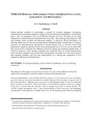
aiding. Braid bars are sediment features found between thesub-streams of multi-thread, braided rivers (Figure 3.7b). Braidbars are highly mobile, and deflection of flow due to bar movementis responsible for the shifting pattern of anabranches and frequentbank attack that characterize braided-river morphology.Figure 3.5 – Typical MeanderingStream with Point BarsFigure 3.6 – Typical Middle Bar28 Fundamentals of Fluvial Geomorphology and Stream Processes

(a) AlternateFigure 3.7 – Typical Bar Patterns(b) BraidedFundamentals of Fluvial Geomorphology and Stream Processes 29

Sinuosity (P) is a commonly used parameter to describethe degree of meandering in a stream. Sinuosity is defined as theratio of distance measured along the stream (stream length) todistance measured along the valley axis (valley length). Aperfectly straight stream has a sinuosity of unity, while a streamwith a sinuosity of 3 or more would have tortuous meanders.Meander wavelength (L) is the straight line repeating distance forthe meander waveform, as depicted in Figure 3.8, and is twice theinflection point spacing. The meander path length is the streamlength between inflection points. Meander amplitude (A) is thewidth of the meander bends measured perpendicular to the valleyor straight-line axis (Figure 3.8). The ratio of the amplitude tomeander wavelength is generally within the range of 0.5 to 1.5.Meander wavelength and amplitude are primarily dependent onthe water and sediment discharge, but are usually locally modifiedby spatial variation in the erodibility of the material in which thestream is formed. The effects of different bank materials areresponsible for the irregularities found in the alignment of naturalstreams. In rare cases where the material forming the banks ispractically homogeneous, meanders take a form that may beapproximated by a sine-generated curve with a uniform meanderwavelength. The meander belt is formed by and includes all thelocations historically held by a stream due to meanderdevelopment and migration. It should be noted that the width of themeander belt is usually greater than the meander amplitude and, inmany cases, may include all of the active floodplain.Figure 3.8 – Definition Sketchfor Stream Geometry (FISRWG1998)The radius of curvature (r c ) is the radius of the circledefining the centerline curvature of an individual bend measuredbetween the bend entrance and the bend exit (Figure 3.8). Thearc angle (θ) is the angle swept out by the radius of curvature.The radius of curvature to width ratio (r c /w) is a very useful30 Fundamentals of Fluvial Geomorphology and Stream Processes

parameter used in the description and comparison of meanderbehavior, and in particular, bank erosion rates. The radius ofcurvature is dependent on the same factors as the meanderwavelength and width. Meander bends generally develop a r c /w of1.5 to 4.5, with the majority of bends falling in the range of 2 to 3.Nanson and Hickin (1986) examined the influence of r c /w on bendmigration rate and reported that maximum bank erosion ratesoccurred when the stream acquired an r c /w of between 2 and 3.This finding has been supported by many empirical studies, forexample, Thorne (1991). Plots of erosion rate versus r c /w do,however, display wide scatter and Biedenharn et al. (1989)showed that part of this scatter could be explained by variations inthe erodibility of the outer bank material (Figure 3.9).Figure 3.9 – Average AnnualErosion Rate versus r/w forMeander Bends of the RedRiver – Open SymbolsRepresent Free, Alluvial Bendsand Closed Symbols,Constrained Bends (developedfrom diagrams by Biedenharn etal. 1989)River slope is one of the best indicators of the ability of theriver to do morphological work and, in general, rivers with steepslopes are much more active with respect to stream changesachieved through sediment movement, bed scour, bar building,and bank erosion. Slope can be defined in a number of ways,however, leading to inconsistency in the way slope is used torepresent the ability of the river to do morphological work. Ideally,the energy slope should be used when calculating stream power,but the data required are seldom available. In gaged streams, thewater surface slope may be calculated using stage readings atconsecutive gaging stations along the stream. However, manysmall streams are ungaged. In ungaged streams, the thalwegslope is often used to calculate stream power. The thalweg profilenot only provides a reasonable basis for calculation of streampower, but may aid in locating bed controls due to geologicFundamentals of Fluvial Geomorphology and Stream Processes 31

outcrops, other non-erodible materials or inputs of relativelyimmobile sediments by steep tributaries. Repeat thalweg profilesare particularly useful in identifying bed level adjustments throughaggradation, degradation, local scour, and fill. When employingdifferent slopes to calculate stream power, it must be kept in mindthat the thalweg, water surface, and energy slopes are notnecessarily equal.3.4 SEDIMENT TRANSPORTOne aspect of river engineering that causes considerableconfusion and misunderstanding is the terminology associated withsediment transport. When discussing sediment transport, it isimportant to be familiar with the terminology adopted and thenature of the load being discussed. Over an extended period, acommon terminology has emerged and while it is not universallyagreed or applied, it does provide the basis for at least reducinginconsistency.Total sediment load is the mass of granular sedimenttransported by the stream. It can be broken down by source,transport mechanism, or measurement status (Table 3.1). Bedload is a component of total sediment load made up of particlesmoving in continuous or frequent contact with the bed. Transportoccurs at or near the bed, with the submerged weight of particlessupported by solid-solid contact with the bed. Bed load movementtakes place by processes of rolling, sliding, and saltation.Suspended load is a component of the total sediment load madeup of sediment particles moving in continuous or semi-continuoussuspension within the water column. Transport occurs above thebed, with the submerged weight of particles supported byanisotropic turbulence within the body of the flowing water. Bedmaterial load is the portion of the total sediment load composed ofgrain sizes that are found in appreciable quantities in thestreambed. The bed material load is the bed load plus the coarserportion of the suspended load, that is, particles of a size that arefound in significant quantity in the streambed. Wash load is theportion of the total sediment load composed of grain sizes finerthan those found in appreciable quantities in the streambed.Measured load is the portion of the total sediment load sampledby conventional suspended load samplers. The sediment sampledin deriving the measured load includes a large proportion of thesuspended load, but excludes that portion of the suspended loadmoving very near the bed (that is, below the sample nozzle) and allof the bed load. Unmeasured load is that portion of the totalsediment load that passes beneath the nozzle of a conventionalsuspended load sampler, moving in near-bed suspension and asbed load.32 Fundamentals of Fluvial Geomorphology and Stream Processes

Table 3.1 – Classification of theSediment LoadMeasurementmethodTransportmechanismSedimentsourceUnmeasured LoadBed LoadBed Material LoadMeasured LoadSuspended LoadWash Load3.5 CHANNEL-FORMINGDISCHARGEMorphological studies have revealed that channel formdepends on a delicate balance between the flows of water andsediment that shape the stream, the processes by which channelform is changed, and the ability of the boundary materials to resistchange. Variability of the water and sediment discharges is acharacteristic of the watershed and, if maintained over asufficiently long period, the morphology of the stream will adjust toaccommodate the range of flow events responsible for regulatingthe balance between the erosive and resistive forces that mold thestream. Consequently, the shape and dimensions of an alluvialriver channel are adjusted to and reflect the wide range of flowsthat entrain, transport, and deposit boundary sediments (Lane1955). The concept that there is a single discharge which, if itprevailed all the time, would produce the same width, depth, slope,hydraulic roughness, and planform as those produced by theactual range of discharges, is attractive, but viewed in this contextit is clearly a gross simplification. The single discharge best ableto represent the actual spectrum of sediment-transporting eventsto yield the same bankfull morphology as that shaped by thenatural sequence of flows is referred to as the channel-formingflow or the dominant discharge. Dunne and Leopold (1978)defined stream maintenance flow as the most effective dischargefor moving sediment, forming or removing bars, forming orchanging bends and meanders, and generally doing work thatresults in the average morphologic characteristics of streams.Their definition of stream maintenance flow is very similar to theconcept of channel-forming discharge.In a regulated canal system, the dimensions of the streamcan appropriately be based on a single design discharge andempirical analysis of the relationship between that discharge andthe dimensions for a stable, unlined canal formed in alluvialmaterials produced the regime theory. Early work on regimetheory stems from design of straight canals in the Indian sub-Fundamentals of Fluvial Geomorphology and Stream Processes 33

continent (Inglis 1941, 1947, 1949) and North America (Blench1952, 1957). Later, flume experiments extended the regimeapproach to streams with meandering planforms (Ackers andCharlton 1970a,b). However, for widely varying flows emanatingfrom a natural watershed, the problem of identifying the singlechannel-forming discharge is both challenging and critical.Soar (2000) reviewed the literature pertaining to the concepta channel-forming flow. This concept is closely related to thetheory of dynamic-equilibrium, which is characterized byfluctuations of channel form around an average condition thatpersists through time. In perennial rivers, recovery of equilibriumfollowing a major event occurs relatively quickly, partly becauserapid vegetation growth encourages sedimentation (Hack andGoodlett 1960; Gupta and Fox 1974). Hence, the long-term timeaveragedcondition is a valid representation of channel form.Recovery in the ephemeral streams of semi-arid regions tends totake longer, reflecting the influence of relatively wet and dryperiods on vegetation growth (Schumm and Lichty 1965; Burkham1972). In arid areas, infrequent floods impart long-lasting imprintson the stream because more frequent flows do not have the powerto restore a regime condition (Schick 1974). It has been concludedthat the channel-forming flow concept may be inapplicable toephemeral rivers that exhibit highly variable flow regimes, becausethere may not be a single discharge that can explain channel form(Stevens et al. 1975; Baker 1977). This is the case, becausestream morphology is likely to be perpetually in disequilibrium withthe prevailing flows rather than fluctuating around an averagestate.The channel-forming flow or dominant discharge is actuallya geomorphological concept and not strictly a measurableparameter. However, there are a number of discharges that maybe taken to represent the channel-forming flow and that can bedefined and calculated using prescribed methodologies. The firstapproach is to identify a candidate flow based on streammorphological, such as the bankfull discharge. A second approachis to select a discharge based on a specified recurrence intervaldischarge, typically between the one- and three-year event in theannual maximum series. The third approach is analytical andinvolves calculating the effective discharge.3.5.1 Bankfull DischargeBased on both theoretical and empirical arguments, bankfulldischarge is generally recognized as being the moderate flow thatbest fits Wolman and Miller’s (1960) dominant discharge conceptfor rivers in dynamic equilibrium. Leopold et al. (1964) proposedthat the bankfull discharge was responsible for streammaintenance and form, and, therefore, implied that it is equivalent34 Fundamentals of Fluvial Geomorphology and Stream Processes

to the channel-forming discharge. Dury (1961) also suggested thatthe channel-forming discharge is approximately equal to thebankfull discharge and Dunne and Leopold (1978) concluded thattheir maintenance discharge corresponded to the bankfull stage.Field identification of bankfull discharge is, however, problematic(Williams 1978). It is usually based on identification of theminimum width to depth ratio (Wolman 1955; Pickup and Warner1976), together with the recognition of some discontinuity in thenature of the stream such as a change in sedimentary orvegetative characteristics. Nixon (1959) defined the bankfull stateas the highest flood of a river that can be contained within thestream without spilling water on the river floodplain. Wolman andLeopold (1957) defined bankfull stage as the elevation of the activefloodplain. Woodyer (1968) suggested that bankfull dischargecorresponds to the elevation of the middle bench of rivers havingseveral overflow surfaces. Schumm (1960) defined bankfull as theheight of the lower limit of perennial vegetation, primarily trees.Similarly, Leopold (1994) states that bankfull is indicated by achange in vegetation, such as herbs, grasses, and shrubs. Finally,the bankfull stage is also defined as the average elevation of thehighest surface of the stream bars (Wolman and Leopold 1957).Harrelson et al. (1994) provide explanations of field methods forfield-determining bankfull discharge using vegetation, gradation ofbank materials, and elevation of sedimentary features. Althoughseveral criteria have been identified to assist in field identificationof bankfull stage, ranging from vegetation boundaries tomorphological breaks in bank profiles, considerable experience isrequired to apply these in practice, especially on rivers that have,in the past, undergone aggradation or degradation.3.5.2 Specified RecurrenceInterval DischargeProblems and subjectivity in the field identification ofbankfull elevation and discharge make it attractive to use anobjectively defined discharge such as a specific recurrence intervalflow. This recurrence interval flow can, in turn, be related to thebankfull elevation (Table 3.2). Wolman and Leopold (1957)suggested that the bankfull frequency has a recurrence interval ofone to two years. The most often-quoted recurrence interval is 1.5years. Dury (1973) concluded that the bankfull discharge isapproximately 97% of the 1.58-year discharge, or the mostprobable annual flood. Hey (1975) demonstrated that the 1.5-yearflow (annual maximum series) passed through the scatter ofbankfull discharges along three British gravel-bed rivers. Richards(1982) suggests that, in a partial duration series, bankfulldischarge equals the most probable annual flood, which has a 1-year return period. Leopold (1994) concludes that mostinvestigations have found that the recurrence interval for bankfulldischarge ranges from 1.0 to 2.5 years. However, there are manyFundamentals of Fluvial Geomorphology and Stream Processes 35

instances where the bankfull discharge does not fall within thisrange. For example, Williams (1978) showed that for thirty-fivefloodplains in the United States (US) the recurrence interval ofbankfull discharge varied between 1.01 to 32 years, and found thatonly about a third of those streams had a bankfull discharge with arecurrence interval between 1 to 5 years. In a similar study, Pickupand Warner (1976) determined that bankfull recurrence intervalsranged from 4 to 10 years on the annual series.Table 3.2 – RecommendedFrequencies for BankfullDischarge (after Soar 2000)Discharge frequencyRecommended by1 to 5 years Wolman and Leopold (1957)1.5 year Leopold et al. (1964); Leopold (1994); Hey (1975)1.58 year Dury (1973, 1976); Riley (1976)1.02 to 2.69 years Woodyer (1968)1.01 to 32 years Williams (1978)1.18 to 3.26 years Andrews (1980)1 to 10 years, 2 year USACE (1994)2 years Bray (1973, 1982)If a specified recurrence interval flow is used to estimate thechannel-forming discharge, a range of 1 to 3 years should be used.However, because of the uncertainties discussed above, it isrecommended that discharges in this range be compared tobankfull stage in the field to verify that the discharges do havemorphological significance.3.5.3 Effective DischargeThe effective discharge is defined as the increment ofdischarge that transports the largest fraction of the annualsediment load over a period of years (Andrews 1980). Theeffective discharge incorporates the principle prescribed byWolman and Miller (1960) that the channel-forming or dominantdischarge is a function of both the magnitude of sedimenttransportingevents and the frequency of occurrence. Anadvantage of using the effective discharge is that it is a calculatedvalue integrating discharge and sediment transport regimes of thestream.Equivalence between bankfull and effective discharges fornatural alluvial streams that are in regime has been demonstratedfor a range of river types (sand, gravel, cobble, and boulder-bed),and in different hydrological environments if the flow regime isadequately defined and the appropriate component of the36 Fundamentals of Fluvial Geomorphology and Stream Processes

sediment load is correctly identified (Andrews 1980; Carling 1988;Hey 1997). However, Benson and Thomas (1966), Pickup andWarner (1976), Webb and Walling (1982), Nolan et al. (1987), andLyons et al. (1992) report that the effective and bankfulldischarges are not always equivalent. This suggests that theeffective discharge may not always be a direct surrogate for thechannel-forming flow or the bankfull discharge.Although the effective discharge is straightforwardconceptually, and has been used for many years, many engineershave expressed concerns that the effective discharge calculationsdo not yield reasonable results in some instances. These problemsmay be attributable to data limitations, insufficient understanding ofthe morphology of the stream or to improper calculation procedure.To minimize these uncertainties a standardized procedure for thedetermination of the effective discharge has been developed and isoutlined in the following paragraphs. This procedure is intended tohelp investigators avoid many of the potential problems that theauthors have experienced in the calculation of the effectivedischarge. Interested readers are referred to Biedenharn et al.(2000a) for a more detailed discussion of effective dischargecalculation.The method most commonly adopted for determining theeffective discharge is to calculate the total load (tons) transportedby the range of flows over a period of time by multiplying thefrequency of occurrence of selected discharge classes (number ofdays) by the median magnitude of the sediment load (tons/day)transported by that class of flows. While this approach has themerit of simplicity, the accuracy of the estimate of the effectivedischarge is clearly dependent on the calculation procedureadopted. The basic inputs required for calculation of effectivedischarge are: 1) flow-duration data, and 2) sediment transport asa function of stream discharge.The first step in an effective-discharge calculation is togroup the discharge data into classes and determine the number ofevents occurring in each class during the period of record. This isusually accomplished from a flow-duration curve, which is acumulative distribution function of measured discharges. A flowdurationcurve shows the percent of time a specific discharge isequaled or exceeded during the period of record, for which thecurve was developed. From the flow-duration curve, the number ofdays that discharges within the specified class interval occurredcan be calculated. The three critical components that must beconsidered when developing a flow-duration curve are the timebase, the number of class interval, and the period of record.Conventionally, values of mean daily discharge are used tocompute the flow-duration curve. Although this is convenient andFundamentals of Fluvial Geomorphology and Stream Processes 37

uses readily available mean daily flow data that are published bythe U.S. Geological Survey (USGS), it can in some cases,introduce bias into the calculations. This arises because meandaily values underestimate the influence of the high flows thatoccur within the averaging period and overestimate thesignificance of the low flows. On large streams such as theMississippi River, the use of the mean daily values is acceptablebecause differences between mean daily and the daily peakdischarges are negligible. However, on flashy streams, the timefrom the flood peak to base flow may be only a few hours so thatmean daily flow cannot adequately describe the hydrograph.Missing flood peaks and associated high sediment loads can resultin the effective discharge being underestimated. Rivers with a highflashiness index, defined as the ratio of the instantaneous peakflow to the associated daily mean flow, are most affected.To avoid this problem, it may be necessary to increase thetemporal density of the flow-duration curve from 24 hours (meandaily) to 1 hour, or even 15 minutes, especially on flashy streams.This will ensure that the hydrograph is adequately described,enabling a more representative effective discharge to bedetermined.Class intervals should be arithmetic and must be of equalwidth. It has been demonstrated that the use of logarithmic or nonequalwidth arithmetic classes introduces systematic bias into thecalculation of effective discharge (Soar 2000). However,interested readers should review Holmquist-Johnson (2002) forguidance in calculating effective discharge for conditions underwhich equal width class intervals are not usableThe selection of class interval may influence the calculatedeffective discharge. There are no definitive rules for selecting themost appropriate interval and number of classes. Yevjevich (1972)stated that the class interval should not be larger than s/4, where sis an estimate of the standard deviation of the sample. Forhydrological applications he suggested that the number of classesshould be between 10 and 25, depending on the sample size. Hey(1997) found that 25 classes with equal, arithmetic intervalsproduced a relatively continuous flow frequency distribution and asmooth sediment load histogram with a well-defined peak,indicating an effective discharge that corresponded exactly withbankfull flow. However, in the authors’ experience, 25 classesmay not always produce satisfactory results. It is recommendedthat in difficult cases the number of intervals be increased, but notto the extent that individual classes have zero or only one event.The period of record must be sufficiently long to include awide range of morphologically-significant flows, but not so long thatchanges in the climate, land use, or runoff characteristics of the38 Fundamentals of Fluvial Geomorphology and Stream Processes

watershed produce significant changes with time in the data. Ifthe period of record is too short, there is a significant risk that theeffective discharge will be inaccurate due to the occurrence ofunrepresentative flows. A reasonable minimum period of recordfor an effective discharge calculation is about 10 years, with 20years of record providing more certainty that the range ofmorphologically significant flows is fully represented in the data.Records longer than 30 years should be examined carefully forevidence of temporal changes in flow and/or sediment regimes.The next step in the determination of the effective dischargeis to develop a sediment-rating curve that relates the sedimenttransport and discharge. The sediment-rating curve can bedeveloped from observed, measured sediment loads or using acomputational procedure. Effective discharge is very sensitive tothe slope of the sediment discharge relationship.The sediment load that is responsible for shaping thestream should be used in the calculation of the effective discharge.The suspended sediment load reported by the USGS publicationsusually includes a portion of the bed material load and most of thewash load. If measured suspended sediment data are used for theeffective discharge calculation, then the fine sediment load,consisting of particles not found in appreciable quantities in thebed, should be omitted. If the bed load in the stream is only a smallpercentage of the total bed material load, it may be acceptable touse only the measured suspended bed material load in theeffective discharge calculations. However, if the bed load is asignificant portion of the load, it should be calculated using anappropriate sediment transport function and then added to thesuspended bed material load to provide an estimate of the totalbed material load. If bed-load measurements are available, whichseldom is the case, observed data may be used.Once the wash load has been removed from the data set, asediment-rating curve is developed from the concentration data byplotting the sediment load (concentration times discharge) againstdischarge, and then calculating a best fit regression curve throughthe data, or, as required in some cases, multiple segments of bestfit regression.The discharges used to generate the bed material loadhistogram are the arithmetic mean discharges in each class of theflow-frequency distribution. The bed-material transport rate foreach discharge class is found from the rating-curve equation. Thisload is multiplied by the frequency of occurrence of that dischargeclass to find the total amount of bed material transported by thatdischarge class during the period of record. Care should be takento ensure that the time units in the bed material load ratingequation are consistent with the frequency units for the distributionFundamentals of Fluvial Geomorphology and Stream Processes 39

of flows. The results are plotted as a histogram. The bed-materialload histogram should display a continuous distribution with asingle mode (peak). If this is the case, the effective dischargecorresponds to the mean discharge for the modal class (that is thepeak of the histogram). If the modal class cannot be readilyidentified, the peak of a smooth curve drawn through the tops ofthe histogram bars can be used to estimate the effective dischargeby interpolation.3.5.4 OverviewAll three approaches (bankfull estimate, discharge of aselected return period, or effective discharge) for estimating thechannel-forming flow or dominant discharge present challenges.The selection of the appropriate method will be based on dataavailability, physical characteristics of the study stream, level ofstudy, and time and funding constraints. It is recommended that allthree methods be used and the results cross-checked to reducethe uncertainty in the final estimate of the channel-forming flow. Ifthe effective-discharge method is used, then it is recommendedthat the standardized procedure presented herein be followed.3.6 RELATIONSHIPS INRIVERSGiven the evident complexity of fluvial processes and theinteractions with stream morphology, it is perhaps surprising thatthe characteristic forms adopted by alluvial rivers are limited innumber and are frequent in occurrence. For example, theplanforms of meandering rivers display clear similarity inproportions. Brice (1984) suggested that the similarity of meandersaccounts for the fact that, if scale is ignored, all meandering riverstend to look alike in plan view. It is the familiar and almostubiquitous nature of the forms and features displayed by alluvialstreams of different sizes, in widely varying landscapes, whichmakes these complex systems amenable to description byrelatively simple empirical relationships. For example,relationships developed by Williams (1986) illustrate how Brice’srecognition of the similarity of meanders may be expressedquantitatively through empirical relationships relating the geometricproperties of stream meander to one another (Table 3.3).40 Fundamentals of Fluvial Geomorphology and Stream Processes

Table 3.3 – Meander GeometryEquations (Williams 1986;adapted from FISRWG 1998)EquationNumberEquationApplicableRangeInterrelations between meander features2 L m = 1.25 b 18.0 < L b < 43,600 ft3 L m = 1.63B 12.1 < B < 44,900 ft4 L m = 4.53R c 8.5 < R c < 11,800 ft5 L b = 0.8L m 26 < L m < 54,100 ft6 L b = 1.29B 12.1 < B < 32,800 ft7 L b = 3.77R c 8.5 < R c < 11,800 ft8 B = 0.61L m 26 < L m < 76,100 ft9 B = 0.78L b 18.0 < L b < 43,600 ft10 B = 2.88R c 8.5 < R c < 11,800 ft11 R c = 0.22L m 33 < L m < 54,100 ft12 R c = 0.26L c 22.3 < L b < 43,600 ft13 R c = 0.35B 16 < B < 32,800 ftRelations of channel size to meander features141.53A = 0.0094L m 33 < L m < 76,100 ft151.53A = 0.0149L b 20 < L b < 43,600 ft16 A = 0.021B 1.53 16 < B < 38,100 ft171.53A = 0.117R c 7 < R c < 11,800 ft180.89W = 0.019L m 26 < L m < 76,100 ft190.89W = 0.026L b 16 < L b < 43,600 ft20 W = 0.031B 0.89 10 < B < 44,900 ft210.89W = 0.81R c 8.5 < R c < 11,800 ft220.66D = 0.040L m 33 < L m < 76,100 ft230.66D = 0.054L b 23 < L b < 43,600 ft24 D = 0.055B 0.66 16 < B < 38,100 ft250.66D = 0.127R c 8.5 < R c < 11,800 ftRelations of meander features to channel size26 L m = 21A 0.65 0.43 < A < 225,000 ft27 L b = 15A 0.65 0.43 < A < 225,000 ft28 B = 13A 0.65 0.43 < A < 225,000 ft29 R c = 4.1A 0.65 0.43 < A < 225,000 ft30 L m = 6.5W 1.12 4.9 < W < 13,000 ft31 L b = 4.4W 1.12 4.9 < W < 7,000 ft32 B = 3.7W 1.12 4.9 < W < 13,000 ft33 R c = 1.3W 1.12 4.9 < W < 7,000 ft34 L m = 129D 1.52 0.10 < D < 59 ft35 L b = 86D 1.52 0.10 < D < 57.7 ft36 B = 80D 1.52 0.10 < D < 59 ft37 R c = 23D 1.52 0.10 < D < 57.7 ftRelations between channel width, channel depth, and channel sinuosity38 W = 12.5D 1.45 0.10 < D 59 ft39 D = 0.17W 0.89 4.92 < W < 13,000 ft40 W = 73D 1.23 K -2.35 0.10 < D < 59 ft &1.20 < K < 2.6041 D = 0.15W 0.50 K 1.48 4.9 < W < 13,000 ft & 1.20 < K < 2.60Derived empirical equations for river-meander and channel-size features:A = bankfull cross-sectional area L b = along-channel bend lengthW = bankfull widthB = meander belt widthD = bankfull mean depth R c = loop radius of curvatureL m = meander wavelength K = channel sinuosityFundamentals of Fluvial Geomorphology and Stream Processes 41

Similarly, in regime theory the concept that the width, depth,slope, and planform of a river are adjusted to a channel-formingdischarge is expressed numerically in simple power-law equations.Independent of regime theory, Leopold and Maddock (1953)compiled important statistical equations linking various streamdimensions to discharge using USGS gaging records. Theseequations, termed hydraulic geometry relationships describehow width, depth, velocity, and other hydraulic characteristics varyboth with stage at a station and with changing bankfull dischargedownstream for some streams in the US. The hydraulic geometryrelationships are of the same general form as the regime equationsof Kennedy (1895):where: W = stream width;Q = discharge;D = depth; andV = velocity.W = a Q bD = c Q fV = k Q mLater versions of these hydraulic geometry relationships add themedian bed sediment size (D 50 ) to improve the predictive power ofthe equations, and appear in the following format:W = k 1 Q k2 D 50k3D = k 4 Q k5S = k 7 Q k8D 50k6D 50k9The relationships presented here are only a small sample ofthose available in the literature. Regime relationships areempirical, which means that the relationships are derived fromobserved physical correlations and are strictly only applicable tothe data sets from which the relationships were derived. In thisregard, Rinaldi and Johnson (1997) are correct to point out theinappropriateness of using simple regression equations in thedesign of meander restorations when fluvial processes and streammorphology in the project stream differ manifestly from conditionsin the rivers used to develop the equations. In practice, hydraulicgeometry and other empirical relationships may be widely andusefully applied, provided that conditions in the study watershedare similar to those in the watersheds for which the equations weredeveloped. However, even under ideal conditions these equationsremain incomplete representations of the factors that actually42 Fundamentals of Fluvial Geomorphology and Stream Processes

influence channel form. For example, many popular hydraulicgeometry equations express the stable width solely as a function ofbankfull discharge. If we neglect the effects of vegetation, it wouldbe intuitive that the width of a stream with sandy banks would begreater than that of an equivalent stream with clay banks. Indeed,Schumm's (1960) relationship between width to depth ratio (F) andthe weighted percent silt-clay in the stream perimeter (M) confirmsthis expectation empirically. If Schumm's relationship is valid, awidth equation based only on discharge cannot fully account forobserved width variability. Clearly, the generation of reliable resultsthrough application of simple and imperfect morphological relationsrelies heavily on good insight and sound judgment on the part ofthe individual responsible.A final misapplication of empirical relationships waslampooned by Mark Twain in Life on the Mississippi (Clemens1944). Describing the Mississippi River cutoffs of which he hadknowledge, he conceived a simple empirical relationship betweenriver shortening and time, and then used it to predict the historicaland future lengths of the Mississippi River concluding that:Geology never had such a chance, nor such exactdata to argue from! In the space of 176 years, theLower Mississippi has shortened itself 242 miles.That is an average of a trifle over one mile and athird per year. Therefore, any calm person, who isnot blind or idiotic, can see that in the Old OöliticSilurian Period, just a million years ago nextNovember, the Lower Mississippi River was upwardsof 1,300,000 miles long, and stuck out over the Gulfof Mexico like a fishing rod. And by the same token,any person can see that 742 years from now theLower Mississippi will be only a mile and threequarterslong, and Cairo and New Orleans will havejoined their streets together, and be ploddingcomfortably along under a single mayor and amutual board of aldermen. There is somethingfascinating about science. One gets such wholesalereturns of conjecture out of such a trifling investmentof fact.The primary points of this passage are that, no matter whatthe basis in fact and observation, empirical relationships cannot beextrapolated either backwards or forwards in time, and engineersmust avoid falling into the trap of designing a project based solelyon ...wholesale returns of conjecture out of a trifling investment offact.Fundamentals of Fluvial Geomorphology and Stream Processes 43

3.7 STREAM STABILITY ANDINSTABILITYIn designing river enhancement and stream-rehabilitationprojects, the design engineer must recognize that rivers aredynamic systems, and must consider both, the existing andpossible future stream morphologies, in the design. The problem iscompounded when engineering interventions are planned becausethe future morphology of the stream depends not only on thenatural, or autonomous evolution of the system, but also streamresponse to construction, operation, and maintenance of theproject. For this reason, it is important for the design engineer toacquire a broad understanding of the current stability status of theproject reach and the extended stream network, and to use thisunderstanding to predict the type and extent of adjustments to thefluvial system likely to be triggered by the project. The capability topredict system response to the proposed works is vital in order toensure that the selected enhancement or rehabilitation measureswill work in harmony with both existing and future river conditions.The concept of stream stability status (which incorporatesinstability) builds on the basic geomorphic principles introducedpreviously and may be applied to the river at system and localscales.3.7.1 System StabilityThe geomorphic concept underpinning stability assessmentin rivers is that over time the cross-sectional dimensions andlongitudinal slope of the stream of an alluvial stream adjust so thatthe stream is able to convey the discharges of water and sedimentsupplied from upstream with no net change to hydraulic geometryor planform. On this basis, a stream may be classified as eitherstable or unstable depending on whether the stream has adjustedor is still adjusting to the flow and sediment regimes. Mackin(1948) expressed the stability concept in his definition of thegraded stream:A graded stream is one in which, over a period ofyears, slope is delicately adjusted to provide, withavailable discharge and with prevailing channelcharacteristics, just the velocity required for thetransportation of the load supplied from the drainagebasin. The graded stream is a system in equilibrium.By definition, a graded stream does not have to have astream that is static or fixed and it may exhibit temporarymorphological changes in response to the impacts of extremeevents. Alluvial stream morphology is certain to be affected bymajor floods or protracted periods of low water, but provided thetime taken for moderate events to restore the graded morphology(termed the recovery time) is shorter than the return period for theextreme event (recurrence interval) then the stream may be44 Fundamentals of Fluvial Geomorphology and Stream Processes

considered to be dynamically stable. The key attribute of a gradedstream is that fluvial processes operating under formative flowstend to restore stream morphology to the graded conditionfollowing disturbance, rather than perpetuating or amplifying thechanges imposed by the extreme event. A commonly used term forthis type of stability is dynamic equilibrium.The concept of dynamic equilibrium is inherent to a widelyapplied (and often mis-applied), qualitative relationship foradjustment in alluvial streams proposed by Lane (1955):QS ~ Q s D 50where: Q = water discharge,S = slope,Q s = bed material load, andD 50 = median size of the bed material.This relationship is commonly visualized as Lane's balance(Figure 3.10). Mackin's explanation of how a graded streamresponds to changes in the controlling variables is easily illustratedby Lane's balance, which shows how a change in any of the fourdriving variables will tend to produce a response in the others suchthat equilibrium is restored. When a stream is in dynamicequilibrium, it has adjusted these four variables such that thesediment transported into the reach is also transported out, withoutaggradation or degradation.Figure 3.10 – Lane’s Balance(after E. W. Lane, from Chorleyet al. (1985))Fundamentals of Fluvial Geomorphology and Stream Processes 45

It should be noted that the map coordinates of a gradedstream may change through time as the river reworks thefloodplain through meandering or braiding, provided that the reachaveragedvalues of width, depth, slope, and planform geometry aretime invariant. Indeed, meandering provides an importantmechanism for an alluvial stream to adjust the slope relativelyquickly and without transferring the large amounts of (relativelycoarse) bed sediment necessary to materially alter slope throughaggradation and degradation. Viewed in this context, changes instream length achieved through meander extension and cutoffrepresent a natural adjustment mechanism, and planform changesdo not necessarily indicate disequilibrium. When natural cutoffsoccur, the river may be obtaining additional length elsewherethrough meander growth, with the net result being that the overallreach length, and therefore slope, remains unchanged.In nature, few rivers actually attain a graded conditionbecause the driving variables change through time. The conceptstill has value, however, because it provides an indication of thelikely trend of stream evolution over engineering time scales, whichare generally less than about 50 years. While it is a mistake toassume that a river will be stable or unchanging over this type ofperiod, the concept of dynamic equilibrium gives useful cluesregarding the rates and types of adjustment that may be expectedas the stream evolves towards a graded condition. Also, theproximity of the system to a graded condition gives an indication ofhow the river will respond to engineering interventions and,particularly how sensitive it is to being destabilized. The value ofthe geomorphically stable stream concept establishes a referencepoint for the definition and treatment of morphological instability ata variety of scales.3.7.2 Stream InstabilityStream instability is defined as temporal change in thehydraulic geometry, long profile or planform pattern of the streamdue to inequality between the supply and removal of sediment.Instability is, in a broad sense, inherent to the natural action ofrivers in changing the landscape through eroding, transporting, anddepositing sediment. In fact, the situation where sediment inputexactly matches sediment output (dynamic stability) is actually aspecial case that can strictly occur only in sub-reaches of a fluvialsystem and which cannot persist for long periods.Instability may result when the flow water and transfer ofsediment through the drainage network is disrupted or significantlyperturbed. The fluvial system initially responds to disequilibrium byadjusting stream morphology in ways that tend to restore theprevious equilibrium or graded condition. If stability is restoredthrough process-response that returns stream morphology to the46 Fundamentals of Fluvial Geomorphology and Stream Processes

pre-disturbance configuration (or something essentially similar)then the adjustments involved are restricted to the immediatevicinity of the disruption and, by definition, constitute localinstability. However, if the magnitude of the change to drivingvariables is large, or the river is sensitive to destabilization due tostream characteristics (high stream power, easy availability ofsediment, high erodibility of bed and bank materials, absence ofgeologic or artificial controls) or proximity to a geomorphicthreshold, then morphological adjustments can take the streamtowards a new equilibrium configuration different from predisturbancemorphology. Under these circumstances, systeminstability propagates throughout the stream network and mayspread into the watershed or even into neighboring systems.3.7.3 Local InstabilityLocal instability refers to the stream changes that result fromthe adjustments to the fluvial system inherent to the maintenanceof a dynamically stable configuration. There are three commoncauses of local instability. The first cause is stream response totemporary variations in discharge or sediment flux. Typically,discharge variations occur seasonally, or result from longer periodsof above average or below average precipitation, while sedimentinput varies due to pulsing of sediment between storage andtransport reaches or shifts in upstream stream alignment. Thesecond cause is the series of adjustments that occur when streammorphology is altered by, and subsequently recovers from, theimpact of a rare event such as a flood, drought, wild fire, orearthquake. The third cause is disruption of fluvial forms orprocesses associated with human activity or construction ofinfrastructure in or around the stream that triggers the streamchanges necessary to accommodate the impacts of thatdisturbance within the existing, dynamically stable condition. Localinstability is not symptomatic of significant disequilibrium in thesystem, but this does not mean that the processes of bed scour,bar deposition, and bank erosion associated with local instabilityare limited to a single location or that the consequences arenegligible.A good example of local instability is bankline movementdue to planform evolution in a meandering river. While the reachaverageddynamically stable parameters of hydraulic geometryand slope remain steady, individual bends in a meandering rivergrow, migrate, and are abandoned. On average, streamlengthening through bank erosion along the concave bank ingrowing meander bends is offset by cutoffs at other bends, as partof the natural meandering process. Under these circumstances,problems associated with bank erosion at a bend are amenable tolocal bank protection works provided that the hydraulic geometryFundamentals of Fluvial Geomorphology and Stream Processes 47

and slope of the reach are not significantly altered. However, itshould be kept in mind that the stream may respond to stabilizationof one bend through accelerated morphological activity in adjacentfree bends. Hence, care must be taken to ensure thatmanagement of local instability at one location does not transfer orconcentrate this natural process elsewhere in a way that isdetrimental to the dynamic stability of the system.The causes of local instability are not limited to the stream.This type of instability can also be triggered by activities insurrounding riparian and floodplain areas. For example, a reach ofstream may display local stream widening due to trampling andover-grazing by cattle, while upstream and downstream reachesthat are not directly affected and are to maintain dynamicallystable. In this situation, a local management solution, based onrestricting access by fencing, construction of suitably reinforcedaccess ramps at water points, and reinstatement of the regimewidth are all that are needed to alleviate a site-specific problem.Site-specific instability problems may respond satisfactorily todesign alternatives developed using reference reach techniques.In practice, however, it is not always easy to establishwhether a local instability problem results from and is amenable toa local solution, or is symptomatic of more serious, system-scaleimpacts and adjustments. Even if the engineer suspects that localinstability results from adjustments of the fluvial system to streaminstability, human activities, or watershed land-use changes, theymay lack the authority or resources to address off-site and nonpointcauses. Under these circumstances, the engineer may haveto modify the adopted solution by constructing a local structurewith the capability for it to continue functioning successfully evenwhen system-driven stream adjustments have significantly alteredlocal conditions. For example, local bank stabilization may berequired at the outside of a migrating bend on a river that ispredicted to degrade in the future due to system instabilitydownstream. Ideally, the system-scale problem (degradation)should be addressed directly using one or more grade controlstructures, but this may be institutionally or financially unfeasible.Recognition that the problem is not entirely local is nonetheless stillvaluable, as it allows the engineer to determine the degree ofadditional toe scour protection necessary to ensure that the bankprotection measures can withstand the additional bed loweringassociated with degradation during the design life of the project.3.7.4 System InstabilityAdjustments involved in system instability typically involveaggradation (increasing bed elevation), degradation (decreasingbed elevation), or planform metamorphosis (abrupt alterationfrom one planform pattern to another). The response of an alluvial48 Fundamentals of Fluvial Geomorphology and Stream Processes

stream to an episode of system instability is, in detail, unique tothat stream and the circumstances and timing of the eventsresponsible for destablization. While Channel Evolution Models(discussed later in the section on stream classification) have beendeveloped to characterize commonly observed styles andsequences of adjustment in unstable systems, there is nogenerally applicable model for process-response to systeminstability.Serious engineering and river-management problems oftenresult from stream instability and may include endangerment ofbridges, buildings, roads, and other infrastructure, undermining ofpipeline and utility crossings, accelerated bed and bank erosion,loss of valuable environmental habitats, and increased sedimentloads that adversely impact flood control and navigation channels,water quality, reservoir areas, and wetlands. Figure 3.11 illustratessome common consequences of system instability.The causes of system instability can be grouped into threecategories: downstream factors, upstream factors, and basin-widefactors.Fundamentals of Fluvial Geomorphology and Stream Processes 49

(a) Bed and Bank InstabilityFigure 3.11 – Consequences ofSystem Instability(b) Formation of Gullies in Floodplain50 Fundamentals of Fluvial Geomorphology and Stream Processes

(b) Damage to InfrastructureFigure 3.11. (cont.) –Consequences ofSystem Instability(d) Excessive Sediment Deposition in Lower Reaches of Watershed3.7.4.1 Downstream Factors The stability of a fluvial system can be significantly affectedby changes to downstream base level. Base level refers to thedownstream limit of the stream network, the elevation of whichdefines the datum for measurement of potential energy in thesystem upstream. In sub-critical flow, the water surface elevationat the downstream limit of the stream controls the longitudinalwater surface profile for a stream. Similarly, the bed elevation atFundamentals of Fluvial Geomorphology and Stream Processes 51

the downstream limit of the system represents the origin of thethalweg profile. It follows from these facts that changes in baselevel have strong potential to trigger system instability.Base-level lowering, due to engineering interventions suchas meander cutoffs or channelization (Figure 3.12) triggersprocess-response by locally steepening the slope and increasingbed material transport capacity. As capacity exceeds supply, thebed scours to make up the deficit supply as the stream adjuststhrough degradation. This adjustment may generate only localinstability if armoring stabilizes the bed or a geological controlprevents significant bed lowering. However, if unchecked by alocal stream response or control, a wave of degradation migratesupstream through the system as a headcut or knickpoint. Ifdegradation triggers bank instability, then a wave of streamwidening may follow the headcut, generating further morphologicaladjustments and additional sediment input to the stream. As thedegradational wave moves upstream, the zone of increased slopeand additional sediment production moves with it. Sedimentsupply to the downstream reaches, coupled with local slopereduction due to upstream bed lowering, then triggers aggradation,which also migrates upstream through the system. Subsequently,sediment output and bed elevation at the downstream limit of thesystem display a damped oscillation until, following a number ofcycles of degradation/aggradation, the long profile is adjusted tothe new base level and stability is restored.Figure 3.12 – ChannelizedStream and Abandoned OldChannel52 Fundamentals of Fluvial Geomorphology and Stream Processes

3.7.4.2 Upstream FactorsThe stability of a fluvial system can also be significantlyaffected by changes to upstream reaches that alter thedownstream discharge or sediment supply. The flow regime andsediment load together, constitute the two main driving variablesresponsible for forming and maintaining the stream and it is nosurprise that the stability of an alluvial river may well be disturbedby changes in one or both of these factors. Upstream factors areoften affected by engineering and river-management projects andthe case of river regulation by a dam or diversion structure is acommon cause of downstream channel adjustment that serves toillustrate the types and complexity of system response that mayresult from such changes.Channel response downstream of a dam or diversionstructure depends on the way the works are constructed andoperated. When the structure is built, sediment supplydownstream may be elevated due to disruption of the channel andfloodplain during construction. This may increase supply overtransport capacity, inducing an initial adjustment throughaggradation. However, this response will be absent if appropriatesediment control measures are applied on site. Once the works arecomplete, process-response downstream will depend on thebalance of changes to the water and sediment regimes. Followingclosure of the dam or diversion, sediment is trapped in the poolupstream of the structure. Sediment-free water released from thestructure then scours the bed downstream, generating degradationin the first few kilometers below the dam. Initially, the flush ofsediment produced drives aggradation further downstream, but asthe stream slope immediately downstream of the dam flattens,sediment output decreases and the leading edge of the zone ofdegradation migrates downstream to re-erode recently depositedsediment and sends it further downstream, as an aggradationalwave. This conceptual model of river response to closure of a damhas been observed in many rivers, and yet this pattern ofadjustment is by no means universal. To explain why, it isnecessary to consider the other morphological responses that maydominate adjustment of the fluvial system. For example, if the beddownstream of the dam includes a widely graded, coarse-grainedfraction, bed armoring may limit degradation and stabilize the bedat a steeper slope than that prior to dam construction. The sameeffect may result from the presence of a geological control, whilewidening with limited reduction in bed level may be triggered if thestream banks downstream of the dam are close to the criticalheight for mass instability (Thorne and Osman 1988). If regulationby the dam significantly reduces the magnitude or frequency ofsediment transporting flows, degradation may be limited ornegligible, and if a reduction in the competence of the main streamis coupled with the input of a substantial sediment load fromunregulated tributaries, aggradation may occur downstream of theFundamentals of Fluvial Geomorphology and Stream Processes 53

dam, where degradation was expected (Biedenharn 1984). Thepoint of citing these examples is to demonstrate that morphologicalresponse to change in one or more upstream factors is complexand difficult to predict. The specific attributes of system instabilityand stream response depend not only on the magnitude ofchanges imposed on the flow regime and sediment loads, but alsoon the sensitivity and boundary conditions of the downstreamchannel network.3.7.4.3 Basin-wide FactorsIn morphological studies, the flow regime and sediment loadare often cited as the independent variables controlling channelform and process. In reality, these variables are not trulyindependent, but depend in turn on the characteristics of thewatershed including factors such as climate, rainfall-runoffrelationship, natural vegetation, land use, and resourcemanagement. Even if upstream and downstream factors remainconstant, changes in the watershed may trigger instability in thefluvial system that leads to widespread morphological adjustments.For example, urbanization can increase peak flows and reducesediment delivery to the stream network. These changes wouldreinforce one another (see Lane’s balance in Figure 3.10) to drivemarked degradation in the stream draining the urbanized area,with morphological impacts migrating upstream and downstreamthrough the system by slope adjustment and sedimenttransmission, respectively. Afforestation of the headwaters of astream could produce very different morphological adjustmentsdepending whether fluvial processes responding more strongly todecreases in runoff (due to increased consumptive use in thewatershed) or elevated sediment delivery (due to erosion alongforestry roads and ditches). In practice, it is even more difficult topredict the morphological response of a fluvial system to basinchanges than to upstream changes. In attempting to develop thecapability to predict stream response to basin-wide changes,engineers and river managers should make every effort tofamiliarize themselves with the geography of the basin, processesoperating in the fluvial system, sedimentary features, and streammorphology. This knowledge, together with application ofconventional hydrologic, hydraulic, and sediment transportanalyses, represents the currently best option for regionalsediment management and stream stabilization in a changingwatershed.3.8 CHANNELCLASSIFICATIONThe existence of a few distinctive channel forms providesthe rationale for morphological classification of channels. Therelationships linking channel form to fluvial process suggests thatthe morphological classification of a channel may allow the54 Fundamentals of Fluvial Geomorphology and Stream Processes

morphologist to infer process from classified channel form. Thefirst step in classification is to identify whether the channel is eitheralluvial or non-alluvial. An alluvial channel flows in bed and banksthat are composed of material transported by the river underpresent flow conditions. The channel is, therefore, free to adjustdimensions and location in response to changes in flow andsediment load. Conversely, a non-alluvial river is neither selfformednor free to adjust. Examples of non-alluvial rivers includebedrock-controlled channel and streams flowing over very coarseglacial deposits.Many classification schemes rest on channel planformpattern, and stem from Leopold and Wolman’s (1957) classificationof channel planforms as straight, meandering, or braided. In thisrespect, the diagram produced by Brice (1975) is notable becauseit builds on earlier schemes to cover a wide range of commonlyobserved planforms, and has proved useful in engineeringgeomorphic studies (Figure 3.13). Schumm (1981, 1985)recognized an even broader range of channel patterns, althoughthe basic straight, meandering, and braided patterns are stillrecognized within his classification of 14 basic patterns (Figure3.14).Fundamentals of Fluvial Geomorphology and Stream Processes 55

Figure 3.13 – Channel PatternClassification Devised by Brice(1975)56 Fundamentals of Fluvial Geomorphology and Stream Processes

11 6 112 7 213 8 314 9410 5Figure 3.14 – ChannelClassification Based on Patternand Type of Sediment Load(after Schumm 1981)Knighton (1998) related Schumm’s 14 patterns toinvestigations by Carson (1984a,b), Knighton and Nanson (1993),and Nanson and Knighton (1996). Knighton (1998) noted that thepatterns in Figure 3.14 are related to the classification by the typeof sediment load (Schumm 1976): bed load, mixed load, andsuspended load. Types 1 through 5 are bed load streams, Types6 through 10 are mixed load streams, and Types 11 through 14 aresuspended load streams. Carson (1984a,b) specified two types ofwandering, gravel-bed rivers. The first is characterized by veryrapid bend migration and frequent chute cutoffs of point bars,similar to Type 3. A second wandering-type is similar to Type 14,with vegetated islands separating most of the channels. Knightonand Nanson (1993) point out that coarse-grain, anastomosingchannels do exist. Therefore, despite the variety of channelpatterns that have been investigated and discussed, a continuumof channel patterns does exist and these patterns are controlled bythe interaction of a series of continuous variables. Figure 3.14suggests some of the variables that should be considered, such assediment size and transport mechanism, while Bledsoe’s (1999)logistic threshold approach indicates that specific stream power,relative strength of the bed and bank materials, and sediment sizeare also important (Figure 3.2).In parallel with the development of his morphologicalclassification, Schumm (1977) considered the type of sedimentload being transported by the stream, the percentage of silt andclay in the channel bed and banks, and the stability of the channelto describe the morphology associated with stable conditions andthe morphological changes expected in response to instabilitythrough aggradation or degradation (Table 3.4). For purposes ofthis classification system, a stable channel complies with Mackin'sFundamentals of Fluvial Geomorphology and Stream Processes 57

definition of a graded stream in which slope is adjusted to supplyjust the sediment transport capacity necessary to convey thesediment load supplied from upstream. An unstable stream maybe either degrading (eroding) or aggrading (depositing). It is veryimportant to remember that the work on which this classificationwas based was conducted in the Midwestern US during thesecond half of the twentieth century. Extrapolation or transfer ofthe classification or related implications to other times and placesshould, therefore, be done cautiously.Table 3.4 – Classification ofAlluvial Channels (after Schumm1977)Mode ofsedimenttransportand type ofchannelSuspendedloadChannelsediment(M)(percent)Bed load(percentageof totalload)Stable(graded stream)>20 10,40;sinuosity usually

Other more ambitious stream classifications have beendeveloped by Neill and Galay (1967), Rundquist (1975), andRosgen (1994). These classifications go well beyond a descriptionof channel form to include description of land use and vegetation inthe basin, geology of the watershed, hydrology, channel bed andbank materials, sediment concentration, channel pattern, andchannel stability.Rosgen (1994) presented a stream-classification systemsimilar to the earlier Rundquist (1975) system. Rosgen (1996)included classification of valley type and introduced anentrenchment ratio, defined as the ratio of the width of the floodpronearea to the surface width of the bankfull channel. Table 3.5is a summary of delineative criteria for broad-level classificationfrom Rosgen (1994). Each of the stream types can be associatedwith dominant bed material types as follows: bedrock – 1, boulder– 2, cobble – 3, gravel – 4, sand – 5, and silt/clay – 6.Table 3.5 – Summary ofDelineative Criteria for BroadlevelClassification (Rosgen1994)StreamtypeEntrench.ratiow/dRatio Sinuosity SlopeMeander belt/bankfull widthDominant bedmaterial*Aa+ 2.2 >12 >1.4 < 0.02 4.0 - 20 1,2,3,4,5,6D na >40 na < 0.04 1.0 - 2.0 3,4,5,6DA >4.0 2.2 1.5 < 0.02 20 - 40 3,4,5,6F 12 >1.4 < 0.02 2.0 - 10 1,2,3,4,5,6G

midwestern experience, while Rosgen's experience began insteep, mountain streams. In addition, Schumm's (1977)classification does not specifically include incised channels, whichare included in Rosgen's (1994) F and G classes. Figure 3.15includes C, D, DA, and E classes, and could be expanded toinclude all of Rosgen (1994) classes. The point of Figure 3.15 is todemonstrate that moving from class to class is a somewhatpredictable morphological response that manages energy,materials, and channel planform to re-establish the balancebetween the local capacity of the channel to convey water andsediment, and the discharge and supply of sediment fromupstream.Figure 3.15 – ChannelClassification CombiningAspects of Schumm (1981)and Rosgen (1994)Thorne et al. (1997) point out that many classificationsystems fail to account for dynamic adjustment or evolution of thefluvial system. Downs (1995) developed a comprehensive systemthat incorporates the classifications of Brice (1975) and Brookes(1981), and builds on their earlier work by linking observed trendsand patterns of adjustment to the fluvial and sediment processesresponsible for driving channel change (Figure 3.16). Adjustmentbasedclassifications like that of Downs differ fundamentally frommorphology-based schemes in that each system requires theobserver to determine the current stability status of the channeland the nature of channel adjustment processes. Because datamay not be available to document change, these schemes requiresound judgment on the part of the engineer, who must inferprocesses and trend of adjustment from channel form.60 Fundamentals of Fluvial Geomorphology and Stream Processes

Figure 3.16 – Downs’ ChannelClassification, Based on Trendsand Types of MorphologicalChange (modified from Downs1995)Although any conceivable morphological channelclassification will oversimplify the variability of channel patterns innature, the underlying concepts of a continuum of channel patternsthat is related to a limited number of controlling variables remainvalid. The opportunity and the challenge for the river engineer is todevelop and refine associations between channel patterncharacteristics and controlling variables, and to use theserelationships with care and caution to predict the manner in whichpattern will change in response to alteration of controllingvariables. Schumm (1976) points out that major alterations inpattern change, which he termed channel metamorphasis, may betriggered by a relatively minor change in a controlling variable, ifthe existing pattern is near a geomorphic threshold.3.9 CHANNEL EVOLUTIONMODELSNumerous geomorphologic studies have used datadeveloped from different locations to infer landform developmentthrough time, commonly employing a technique termed locationfor-timesubstitution. This technique assumes that by observingchannel form as one moves downstream along a channel, theeffect of physical processes at one location through time can bepredicted; that is, changing location is substituted for changingtime. This technique was used to develop a Channel EvolutionModel (CEM) for Oaklimeter Creek, an incised stream in northernMississippi (Schumm et al. 1981, 1984). Simon and Hupp (1987)later developed a similar model of channel evolution based onFundamentals of Fluvial Geomorphology and Stream Processes 61

Schumm et al. (1981, 1984) and their observations of incisedstreams in western Tennessee.The CEM (Figure 3.17) consists of five channel-reach types,which describe the evolutionary phases typically encountered in anincised channel. These evolutionary phases range from strongdisequilibrium to a new state of quasi-equilibrium. Quasiequilibriumimplies that the system is not static and changesthrough time, but over a period of years the average condition isone of stability. The model is based on the assumption thatmoving downstream through the system is equivalent to remainingin place and monitoring changes due to the passage of time. Theresponse at any given location in the channel can then bepredicted from the morphology of downstream channel locations.The channel reach types in the CEM are labeled Types Ithrough V, and are assumed to occur consecutively in thedownstream direction. The CEM assumes each channel type willoccur in turn at a given location as the channel evolves. The CEMchannel types are illustrated in Figure 3.17. Type I reaches arelocated upstream of the actively degrading reach and have not yetexperienced significant bed or bank instabilities. These reachesare generally characterized by U-shaped cross sections with littleor no recently deposited sediment stored in the channel bed.Type II reaches are encountered immediately downstreamof Type I reaches. Bed degradation is the dominant process inthe Type II reach. Type II channels are over-steepened reacheswhere the sediment transport capacity exceeds the sedimentsupply. Although the channel is actively degrading in a Type IIreach, the bank heights (h) do not exceed the critical bank height(h c ), and therefore, reach-scale geotechnical bank instability is notencountered.62 Fundamentals of Fluvial Geomorphology and Stream Processes

Figure 3.17 – Incised ChannelEvolution Sequence (afterSchumm et al. (1984))As bed degradation continues, the bank heights and anglescontinue to increase. When the bank heights exceed the criticalbank height for stability in Type III reaches, mass failures(geotechnical instability) begin. The dominant process in the TypeIII reach is channel widening. In places, the Type III reach maycontinue to be slightly degradational. However, the reducedsediment transport capacity resulting from the longitudinal channelslope decreasing combined with increased sediment supply fromupstream due to instability and from bank failures within the reachoften results in the initiation of sediment deposition on the channelbed.Type IV reaches are downstream of Type III reaches andrepresent the first manifestation of the incising channel returning toa new state of dynamic equilibrium. In the Type IV reach,geotechnical bank instabilities and channel widening may continue,Fundamentals of Fluvial Geomorphology and Stream Processes 63

ut at a much reduced rate. The sediment supply from upstream(Type III) exceeds the sediment transport capacity, resulting inaggradation of the Type IV channel bed. The Type IV reach is alsocharacterized by the development of berms, which aredepositional features along margins of the over-widened channel.These berms represent the beginning of a new inner channel withdimensions adjusted to the flow and sediment regime.Type V reaches represent a state of dynamic equilibriumwith a balance between sediment transport capacity and sedimentsupply. Bank heights in the Type V channel are generally less thanthe critical bank height, and therefore, reach-scale geotechnicalbank instability ceases. However, local bank failures can still existas part of the meander process, or as the results of constrictions,obstructions, or other local factors. The berms, which wereinitiated in the Type IV reach have now become colonized byriparian vegetation forming a compound channel within the larger,incised channel. The equilibrium channel of Type V is of acompound shape, with a smaller inner channel bounded by anarrow floodplain. The original floodplain of the Type I channel isnow a terrace.The CEM addresses the channel stability status within asystem context. Dynamic equilibrium in a Type V reach simplyimplies that system stability has been attained. A Type V reachmay exhibit considerable erosion that is part of the naturalmeander process or some other local process, yet still be classifiedas being in dynamic equilibrium.The primary value of the CEM sequence is to underpinidentification of the evolutionary state of the channel from fieldreconnaissance. The morphometric characteristics of the channelreach types can also be correlated with hydraulic, geotechnical,and sediment transport parameters (Harvey and Watson 1986;Watson et al. 1988). The evolution sequence provides anunderstanding that while reaches of a stream may differ markedlyin appearance, the channel form in one reach is associated withthat in adjacent and remote reaches by an evolutionary process.Form, process, and time relate dissimilar reaches of the streamlinked to complex response and connectivity in the water andsediment transfer systems.3.10 GEOMORPHICASSESSMENTHaving recognized the significance of fluvial geomorphologyto engineering and management of rivers, the problem remains ofgathering the data and qualitative information necessary tocharacterize and define channel form, process, and stability statusin the project river. A thorough geomorphic assessment of theriver and watershed is required. Unfortunately, many engineers64 Fundamentals of Fluvial Geomorphology and Stream Processes

charged with the design of river projects either fail to fullyappreciate the importance of geomorphic assessments, or lack theeducation or training background to perform them adequately.Geomorphic assessment is an essential part of the designprocess for schemes ranging from local bank protection, throughreach-scale habitat enhancement, to master planning for waterresource management in an entire watershed. The aims ofgeomorphic assessment are to provide the baseline informationnecessary to characterize process-form interactions in the river,identify control points and problem reaches, and support division ofthe system into geomorphically distinct sub-reaches that may beindividually classified with respect to morphology. Once thesystem has been characterized and classified, the engineer mayassess the stability status on a reach-by-reach basis and predictthe medium and long-term autonomous evolution under a donothing scenario. This provides a base line against which toassess the morphological responses of the project reach and widersystem to the proposed engineering, rehabilitation, or waterresources project.Perhaps the most important step in any geomorphicassessment is ensuring that the scope and content match theproject goals, authority, stream and watershed characteristics, andavailable resources. There is no standardized or cookbookapproach, but over the last two decades a number of assessmentschemes have been developed and these provide valuableguidance based on direct experience (Schumm et al. 1984;Richardson and Huber 1991; Schall and Lagasse 1991; Shiroleand Holt 1991; Biedenharn et al. 2000b; Robinson and Thompson1993). Typically, existing geomorphic assessment techniques maybe sub-divided into procedural steps dealing with:• assembly of existing and archived data/information in adesk study;• establishment of current channel forms and sedimentfeatures through stream reconnaissance and fieldsurveys;• geomorphic analysis and interpretation of historical andcontemporary information;• stream classification and assessment of stability status atreach scale;• prediction of past and future morphological evolution andresponse to proposed project; andFundamentals of Fluvial Geomorphology and Stream Processes 65

• integration of results into engineering design to optimizeperformance.For more detailed reviews of practical and procedural issuesin geomorphic studies and assessment, the reader is referred toarticles by the third author (Thorne 1998, 2001).The results of geomorphic assessments are rarely clear cut.More often, the individual elements of the assessment produceoutcomes that are equivocal or even contradictory. For example,the specific gage record for a hydrological station may indicate thatstages for a given discharge have decreased significantly, whilethe few available repeat cross sections from the same period showvariations in bed topography but no evidence for discerniblechange, and stream reconnaissance indicates that the stream ishydraulically connected to the floodplain. The specific gagerecords suggest that the stream has degraded, but there is a lackof supporting evidence from resurveyed cross sections and streamreconnaissance that the streambed and floodplain levels aremutually-adjusted. In these situations, a level of confidence mustbe assigned to morphological conclusions based on differentcomponents of the assessment, based on the quantity, quality, andreliability of the data and the assessor’s experience in applying thetechniques involved. It may then be possible to reconcileapparently contradictory results by weighing the levels ofconfidence associated with each one. It is emphasized soundjudgment, based on insight and experience, that is essential foraccurate geomorphic assessment.Obviously, geomorphic assessment alone can neverprovide a proper basis for engineering analysis or design. It is,however, of value when combined with computational andanalytical methods for stable stream design. The widercontribution provided by geomorphic assessment is to establishthe system context and framework within which the designer may:• select hydrodynamic and sediment transport equationsappropriate to the stream and conditions;• match design of stable stream dimensions that mimicnatural channel forms and diversity while meeting projectgoals;• use computer models matched to the alluvial setting andincorporating existing geologic and artificial controls topredict morphological response of the stream system toproposed rehabilitation measures;• integrate environmental features effectively intomorphological and engineering aspects of the project;66 Fundamentals of Fluvial Geomorphology and Stream Processes

• anticipate maintenance requirements and optimize thedesign to ensure that the benefits are sustainable; and• consider and propose the scope of a Post-ProjectAppraisal (PPA) and monitoring regime necessary toestablish the strengths and weaknesses of projectperformance.Geomorphic assessment alone is not sufficient to guaranteethat a project will perform adequately with regard to morphologicaland environmental goals, but it is a valuable and necessarycomponent of the integrated stream design process that isessential to ensure long-term sustainability in river engineering andmanagement projects.3.11 SUMMARYFluvial geomorphology, analytical river mechanics, andsound engineering judgment together provide the foundations forsound river engineering, rehabilitation, and management. Insightsand understanding provided by geomorphic principles andidentification of causal links between channel form, fluvialprocesses, and connectivity of the river system can be invaluablein the design of river projects and management strategies. This isthe case, not only because the engineering-geomorphic approachis consistent with environmental goals such as minimizing negativeimpacts and maximizing biodiversity, but also because solutionsthat recognize and deal with the causes rather than the symptomsof stream problems represent better engineering. Manyengineering stabilization and rehabilitation projects have failed, notas the result of deficient hydraulic or structural design, but ratherbecause the significance of geomorphology to the project and theproject to geomorphology have not been identified and accountedfor in the design. Experience is accumulating that engineeringdesigns guided by knowledge of the fluvial system are able toavoid having to attempt to ‘tame the river,’ instead working with theriver to produce schemes that have lower long-term maintenancerequirements. Engineering-geomorphology thereby opens thedoor to cost-effective, sustainable solutions that do not commitfuture generations to heavy and expensive maintenance.Fundamentals of Fluvial Geomorphology and Stream Processes 67

68 Fundamentals of Fluvial Geomorphology and Stream Processes