A practical introduction to nordpred - cancerview.ca

A practical introductionto nordpredMichael OtterstatterCancer SurveillanceCentre for Chronic Disease Prevention and ControlPublic Health Agency of CanadaMarch 7-9, 2011

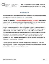
ProjectionsAccurate projections are essential for planning……but how best to predict future events?2

Projections?3

Many models are available• Poisson regression (classic APC model)• other generalized linear models (power models)• generalized additive models• simple average methods• univariate (ARIMA) & multivariate (VAR) time series• state-space models (American Cancer Society)• functional data analysis• Bayesian models (versions of all of the above)4

Practical introduction to nordpredThis presentation is a practical introduction to one approachto projections: the nordpred package for cancer projectionsObservedvaluesNORDPREDProjectedvaluesTheoretical and philosophical considerations are important,but will not be covered here5

The nordpred package• R software package that predicts trends in cancer incidenceusing a version of the traditional age-period-cohort model• written by Harald Fekjær (harald.weedon-fekjaer@kreftregisteret.no)and Bjørn Møller (bjorn.moller@kreftregisteret.no), of the CancerRegistry of Norway• background and example:• Møller B, et al. 2003. Prediction of cancer incidence in the Nordiccountries: Empirical comparison of different approaches. Statistics inmedicine 22:2751-2766• Møller B, et al. 2002. Prediction of cancer incidence in the Nordiccountries up to the year 2020. European Journal of Cancer Prevention11, suppl. 16

The nordpred packageAvailable free-of-charge (but see license agreement):www.kreftregisteret.no/en/Research/Projects/Nordpred/Nordpred-software/# Nordpred: R (www.r-project.org) & S-PLUS# (www.insightful.com) functions# for prediction of cancer incidence (as used in the# Nordpred project)# Written by: Bjørn Møller and Harald Fekjaer# , 2000-2003# Version 1.1. updated to correct for wrong estimates# in young age groups# License: GNU version 27

Recent examples of nordpred• Coupland, V. H. et al. 2010. The future burden of cancer in London comparedwith England. Journal of Public Health, 32:83.• Mork, J. et al. 2010. Time trends in pharyngeal cancer incidence in Norway1981-2005. Cancer Causes and Control, 21:1397• Parkin, D. M. et al. 2009. The potential for prevention of colorectal cancer inthe UK. European Journal of Cancer Prevention, 18:179.• Aitken, R. et al. 2008. Cancer incidence and mortality projections in NewSouth Wales, 2007 to 2011. Cancer Institute NSW.• Olsen, A. H. et al. 2008. Cancer mortality in the United Kingdom: Projectionsto the year 2025. British Journal of Cancer, 99:549.• Parkin, D. M. et al. 2008. Predicting the impact of the screening programmefor colorectal cancer in the UK. Journal of Medical Screening, 15:163.• Ferlay, J. et al. 2007. Estimates of the cancer incidence and mortality inEurope in 2006. Annals of Oncology, 18:581.• Møller, H. et al. 2007. The future burden of cancer in England: Incidence andnumbers of new patients in 2020. British Journal of Cancer, 96:1484.• Quinn, M. J. et al. 2003. Cancer mortality trends in the EU and accedingcountries up to 2015. Annals of Oncology, 14:1148.8

Basic steps for using nordpred1. Reading the nordpred package2. Input data3. Generate projections4. Get results5. Plot results6. Explore options9

1. Reading the nordpred packageDownload ‘nordpred.s’ file to preferred working directory andread package in Rsetwd("C:/Documents and Settings/My Documents/nordpred")source("nordpred.s")10

Example #1: Colon cancer in Norway** Data and code for this example available at nordpred website11

2. Input data: structureNumbers of cancer casesPopulation sizesFive-year periodsFive-year periodsFive-year age groups0-45-910-1415-1920-2425-2930-3435-3940-4445-4950-5455-5960-6465-6970-7475-7980-8485+58-62 63-67 68-72 73-77 78-82 83-87 88-92 93-97Five-year age groups0-45-910-1415-1920-2425-2930-3435-3940-4445-4950-5455-5960-6465-6970-7475-7980-8485+58-62 63-67 68-72 73-77 78-82 83-87 88-92 93-97Note: there must be 18 five-year age groups in both the cases/deathsand population data files12

2. Input data: reading in filesCancer cases or deaths, observedindata

2. Input data: reading in files (continued...)14

2. Input data: reading in files (continued...)Population sizes, observed and projectedinpop1

2. Input data: reading in files (continued...)16

3. Producing projections: overview• Producing projections is a two-step process1. fitting a model to the observed data2. generating projections (unknown future values) based on thefitted model• Nordpred allows these steps to be separate or combined1. Separate: use nordpred.estimate andnordpred.prediction functions in sequence2. Combined: use single nordpred function17

3. Producing projections: overview (continued...)• Nordpred fits an APC regression model to the observed dataCases = (Age) + (Period) + (Cohort) + Period‘drift’ or ‘trend’termcategoricalvariablescontinuousvariable• Due to colinearity among age, period and cohort, lineareffects of period and cohort cannot be estimatedsimultaneously— a common linear trend (‘drift’) isestimated instead• Predictions assume future cohort and period effects areequal to last estimated effect in the fitted model18

3. Producing projections: fit modela. Fit APC regression model to input dataest

3. Producing projections: fit model (continued...)20

3. Producing projections: predictb. Generate projected values from fitted modelres

3. Producing projections: prediction outputObserved and predicted valuesX58.62 X63.67 X68.72 X73.77 X78.82 X83.87 X88.92 X93.97 X98.02 X03.07 X08.12 X13.17 X18.220-4 1 0 0 0 0 0 0 0 0 0 0 0 05-9 0 0 0 0 0 0 0 0 0 0 0 0 010-14 1 0 1 1 0 0 0 0 0 0 0 0 015-19 1 0 0 1 3 0 1 3 2 2.2 2.5 2.6 2.520-24 1 4 2 3 3 2 4 3 3.6 3.1 3.4 3.9 425-29 4 1 6 6 6 11 7 7 9.6 9.5 8.9 9.9 11.830-34 13 11 6 12 15 26 14 10 19.9 20.1 19.3 17.5 19.435-39 27 16 18 15 29 22 31 18 24.2 31.1 30.6 28.5 25.940-44 32 37 32 28 40 50 64 71 59.5 51 62.3 59.5 55.445-49 54 75 73 73 75 72 122 112 163 120.5 104.7 122.5 11750-54 66 103 128 139 125 134 185 190 265.7 278.7 210 183.7 212.455-59 105 124 197 210 257 254 230 269 448.5 444 453.9 347.7 311.560-64 189 212 252 283 369 442 446 436 612.6 742.8 738.5 739.5 585.465-69 197 258 303 358 484 603 683 668 785.1 867.2 1047.7 1045.1 1045.470-74 223 286 376 403 554 663 754 880 1003.5 1001 1104.7 1336.8 1356.175-79 192 262 312 402 502 640 775 913 1100.2 1118.9 1121.9 1246 1535.780-84 146 160 215 278 337 415 513 615 780.3 894.6 921.4 937.8 1066.785+ 81 95 122 151 209 278 328 379 549.3 636.6 755.6 830.1 891.6Observed Predicted23

3. Producing projections: prediction outputModel informationPrediction done with:Number of periods predicted (nopred): 5Trend used in predictions (cuttrend): 0 , 0.25 , 0.5 , 0.75 , 0.75Number of periods used in estimate (noperiod): 8P-value for goodness of fit: 0.7Used recent (recent):TRUEP-value for recent: 0.0292First age group used (startuseage): 6First age group estimated (startestage): 524

4. Get results: basic outputa. Projected numbers and rates, with optionspred_num

4. Get results: basic output (continued…)26

4. Get results: basic output (continued…)b. Generate crude and age-standardized ratespredrates_crude

4. Get results: basic output (continued…)crude ratesage-standardizedrates28

4. Get results: basic output (continued…)29

4. Get results: basic output (continued…)c. Generate projected values and export to a file# GENERATE PROJECTED VALUESpred

4. Get results: basic output (continued…)c. Generate projected values and export to a fileFive year age groupFive year periodX98.02 X03.07 X08.12 X13.17 X18.220-4 0 0 0 0 05-9 0 0 0 0 010-14 0 0 0 0 015-19 2.04 2.19 2.53 2.6 2.5520-24 3.59 3.12 3.35 3.88 3.9725-29 8.72 8.18 7.38 8.06 9.4330-34 16.8 16.17 15.01 13.41 14.6235-39 18.55 22.61 21.57 19.83 17.7740-44 56.4 44.87 52.83 49.85 45.8345-49 153.31 110.05 90.47 103.89 98.0450-54 265.49 272.73 202.67 171.14 194.1655-59 461.84 458.36 463.53 354.79 308.7460-64 658.68 789.19 793.43 792.46 628.4965-69 828.27 958.51 1154 1172.51 1169.3870-74 1008.7 1033.45 1198.54 1454.99 1500.8775-79 1100.34 1140.9 1179.74 1380.22 1706.5780-84 742.88 866.72 914.87 964.69 1153.6985+ 529.27 609.17 739.58 836.86 930.531

5. Plot resultsa. Generate plots of crude and/or standardized ratesplot( res,incidence=TRUE,standpop=NULL,agegroups="all",new=TRUE,lty=c(1,2),col=c(1,1),main="Colorectal Cancer",xlab="Period",ylab="Incidence rate")numbers (FALSE) or rates (TRUE)crude (NULL) or age-stand. rates(vector of weights)overlay on current plot (FALSE) orcreate a new plot (TRUE)line types (1=solid, 2=dashed, etc.)and colours (1=black, 2=red, etc.)labels for plot, x-axis and y-axis32

5. Plot results (continued…)Colorectal CancerIncidence rate0 10 20 30 40 50X58.62 X68.72 X78.82 X88.92 X98.02 X08.12 X18.2Period33

5. Plot results (continued…)b. Overlaying plotsplot( res,incidence=TRUE,standpop=NULL,agegroups="all",new=TRUE,lty=c(1,2),col=c(1,1),main="Colorectal Cancer",xlab="Period",ylab="Incidence rate")plot( res, incidence=TRUE, standpop=Canada1991,new=FALSE, lty=c(1,2), col=c(2,2))plot( res, incidence=TRUE, standpop=US2000,new=FALSE, lty=c(1,2), col=c(4,4))legend(9, 10, c("Crude rate","Canada 1991", "US2000"), text.col=c(1,2,4))34

5. Plot results (continued…)Colorectal CancerIncidence rate0 10 20 30 40 50Crude rateCanada 1991US 2000X58.62 X68.72 X78.82 X88.92 X98.02 X08.12 X18.22Period35

Producing projections: using a single function• Producing projections is a two-step process1. fitting a model to the observed data2. generating projections (unknown future values) based on thefitted model• Nordpred allows these steps to be separate or combined1. Separate: use nordpred.estimate andnordpred.prediction functions in sequence2. Combined: use single nordpred function36

6. Exploring nordpred options: overviewprojections

6. Exploring nordpred options: observed periods3 obs. periods (min)7 obs. periods10 obs. periods38

6. Exploring nordpred options: trendCompare projections using recent vs. historical trendproj_recent_trend

6. Exploring nordpred options: trendCompare projections using recent vs. historical trendIncidence Rate of Colorectal CaIncidence rate0 10 20 30 40 50Historical trendRecent trendX58.62 X68.72 X78.82 X88.92 X98.02 X08.12 X18.22Period40

6. Exploring nordpred options: link functionCompare projections using power5 vs. Poisson linkproj_power5

6. Exploring nordpred options: link functionCompare projections using power5 vs. Poisson linkIncidence Rate of Colorectal CaIncidence rate0 10 20 30 40 50 60PoissonPower5X58.62 X68.72 X78.82 X88.92 X98.02 X08.12 X18.22Period42

6. Exploring nordpred options: choose carefully!Incidence of Colorectal Cancer AmonNumber of new cases0 2000 4000 6000 8000 10000Poisson linkPower linkomit oldest obs.use recent trenduse cut-trendincrease cut-trendX58.62 X68.72 X78.82 X88.92 X98.02 X08.12 X18.22Period43

Acknowledgment and disclaimerThe Cancer Surveillance and Epidemiology Networks have beenmade possible through a financial contribution from Health Canada,provided by the Canadian Partnership Against Cancer.The views expressed herein do not necessarily represent the views ofthe Canadian Partnership Against Cancer nor that of Health Canada.44

Supplemental information45

Calculation of predicted rates in nordpredProjections:1. linear trend component2. non-linear cohort component3. fix period to last estimated valueObserved ratesPredicted rates1995-1999 2000-2004 2005-2009exp(A 1 +5⋅D+C 12 +P 5 ) exp(A 1 +6⋅D+C 13 +P 6 ) exp(A 1 +7⋅D+C 13 +P 6 )exp(A 2 +5⋅D+C 11 +P 5 ) exp(A 2 +6⋅D+C 12 +P 6 ) exp(A 2 +7⋅D+C 13 +P 6 )exp(A 3 +5⋅D+C 10 +P 5 ) exp(A 3 +6⋅D+C 11 +P 6 ) exp(A 3 +7⋅D+C 12 +P 6 )exp(A 4 +5⋅D+C 9 +P 5 ) exp(A 4 +6⋅D+C 10 +P 6 ) exp(A 4 +7⋅D+C 11 +P 6 )exp(A 5 +5⋅D+C 8 +P 5 ) exp(A 5 +6⋅D+C 9 +P 6 ) exp(A 5 +7⋅D+C 10 +P 6 )exp(A 6 +5⋅D+C 7 +P 5 ) exp(A 6 +6⋅D+C 8 +P 6 ) exp(A 6 +7⋅D+C 9 +P 6 )exp(A 7 +5⋅D+C 6 +P 5 ) exp(A 7 +6⋅D+C 7 +P 6 ) exp(A 7 +7⋅D+C 8 +P 6 )exp(A 8 +5⋅D+C 5 +P 5 ) exp(A 8 +6⋅D+C 6 +P 6 ) exp(A 8 +7⋅D+C 7 +P 6 )