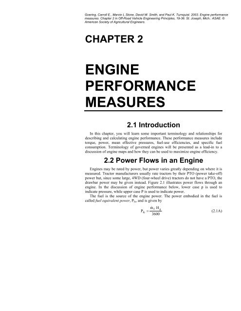
CHAPTER 2 ENGINE PERFORMANCE MEASURES 2.1 Introduction

22 CHAPTER 2 ENGINE PERFORMANCE MEASURESwhereP b = brake (flywheel) power, kWT b = engine brake torque, N.mN e = engine speed, rpmThe significance of the term, brake torque, will be explained a little later. The 60,000in the denominator is simply a units constant. Continuing the above example, assumethe brake torque was 625 N.m. Then Equation 2.4 shows that the brake power of theexample engine was 144 kW.For the example, the engine consumed 375 kW of fuel equivalent power but hadonly 169.4 kW of indicated power at the head of the pistons and only 144 kW of brakepower at the flywheel. The loss, 375 – 169.4 = 205.6 kW, is primarily caused bythermodynamic limitations imposed by the second law of thermodynamics. However,the loss, 169.4 – 144 = 25.4 kW, is due to friction losses in the engine. Friction poweris given byP = P − P(2.5)fiwhere P f = friction power, kW.Thus, by definition, friction power includes any part of the indicated power that isnot delivered to the flywheel. In our example engine, the friction power would be 25.4kW. What is included in friction power? It includes friction in the rings, bearing, etc.However, it also includes power to run the oil pump, cooling fan, alternator, and, foran air-conditioned vehicle, power to run the compressor. A practical consequence ofEquation 2.5 is that, during an official test, turning off the air conditioner reduces thefriction power and adds to the brake power.2.3 Mean Effective PressuresThe term, indicated mean effective pressure, came about at follows. In the earlydays of engine testing, a cylindrical chart was attached to the front of the engine anddriven at crankshaft speed. An inked stylus, driven by a pressure transducer in theengine cylinder, produced a graph of cylinder pressure versus crankshaft rotation.Such a diagram was called an “indicator diagram.” By knowing the ratio of connectingrod length over crank throw radius, it was possible to convert the indicator diagram toa p-v diagram similar to the one in Figure 2.2. The area within the p-v diagram,divided by the base width of the diagram, gives the indicated mean effective pressure.The base width of the diagram is simply the displacement of a single cylinder, D c .More modern methods have replaced the use of the indicator diagram in preparing p-vdiagrams, but the term indicated mean effective pressure is still used in engine theory.In modern testing, a pressure transducer continuously measures the cylinder pressurewhile an encoder measures the crankshaft rotational position. The data are fed into acomputer that calculates the p ime .b

OFF-ROAD VEHICLE ENGINEERING PRINCIPLES 23Figure 2.2. Engine p-v diagram and indicated mean effective pressure.For an engine of displacement D e running at a given speed, N e , Equation 2.2 showsthat the indicated power varies proportionally with the indicated mean effectivepressure. Engine analysts have used a variation of Equation 2.2 to develop other meaneffective pressures. Thus, a brake mean effective pressure, p bme or bmep, can becalculated by120,000 Pbpbme= (2.6)DeNewhere p bme = brake mean effective pressure, kPa.The p bme does not exist as an actual pressure in the engine and thus cannot bemeasured. It can be calculated using Equation 2.6 if the engine displacement, speedand brake power are known. By combining Equations 2.4 and 2.6 and simplifying, thefollowing equation can be derived:DepbmeTb =(2.7)4πThe denominator in Equation 2.7 would be 2π for a two-stroke cycle engine. Brakemean effective pressure is often referred to as specific torque; it is proportional tobrake torque but is independent of the engine displacement. For our example engine,either Equation 2.6 or Equation 2.7 shows the bmep would be 1020 kPa.

26 CHAPTER 2 ENGINE PERFORMANCE MEASURESFigure 2.3. Illustration of governor action.Mechanical governors of the type shown in Figure 2.3a can be a separate unit or, onCI engines, can be included in the fuel injector pump housing. In either case, thegovernor shaft speed is proportional to the crankshaft speed of the engine. As enginespeed increases, increased centrifugal force on the hinged flyweights causes them toswing outward, thus pushing downward on the thrust bearing and causing the linkageto rotate counterclockwise and stretch the governor spring. The fuel control rod thenmoves to decrease fuel delivery to the engine. Conversely, if the engine speed falls,

OFF-ROAD VEHICLE ENGINEERING PRINCIPLES 27the spring causes the linkage to rotate clockwise, pushing the thrust bearing upwardand forcing the flyweights to move inward. The rotating linkage also moves the fuelcontrol rod to increase fuel delivery to the engine. All mechanical governors include athrust bearing because the governor flyweights are attached to a rotating governorshaft, while the pivot of the linkage is stationary; therefore, the bearing accommodatesthe relative motion between the rotating and non-rotating parts of the governor. Thefuel control rod could change fuel delivery in a number of ways. In some SI engines,the rod would control fueling by opening or closing the throttle plate in a carburetor.In CI engines, rod movement would change the delivery of a fuel injection pump. Fuelinjection pumps are discussed in Chapter 7.When the governor is in equilibrium, the force imposed on the thrust bearing by theflyweights is equal to the force imposed by the governor spring. It is helpful inunderstanding governor action to calculate the force on the thrust bearing. FromNewton’s second law, the force on the thrust bearing is2Ftb= K r N g(2.15)whereK = a units constant also incorporating mechanical advantage of flyweight linkager = radius from center of governor shaft to center of flyweightsPlotting thrust-bearing force versus engine speed (Figure 2.3b) leads to the problemthat the radius, r, is changing as speed changes. Two limiting cases have been plottedin the figure, one for weights in (minimum r) and one for weights out (maximum r).Now consider an engine running without load but with substantial fuel delivery.The governor prevents the engine from accelerating until it destroys itself; as speedincreases, the flyweights swing to the full-out position to reduce the fuel delivery andlimit the engine speed to that shown at Point A of Figures 2.3b and 2.3c. Point A iscalled the high idle point because the speed is high and the engine is idling, i.e., notdoing any work. Now imagine that increasing torque load is placed on the engine; theresulting decline in speed causes the flyweights to move inward, thus increasing fueldelivery to the engine to accommodate the increased load. When the torque reachesand exceeds that shown at Point C in Figure 2.3c, the governor flyweights would be attheir innermost position and the linkage would not be able to move the fuel control rodany farther. Point C is called the governor’s maximum point because the governor isunable to affect fuel delivery beyond that point. To the left of Point C in Figure 2.3c,the speed is controlled entirely by the amount of torque load placed on the engine, i.e.,higher loads cause lower engine speeds. Figure 2.3c is called the engine map. The areato the right of Point C on the map is called the governor-control region, while the areato the left is called the load-control region. Although a perfect governor wouldmaintain constant speed in the governor-control region, actual governors permit somespeed variation. Governor regulation, as calculated using Equation 2.16, is a measureof how closely the governor can maintain constant speed.NHI− NGMReg = 200 ( )(2.16)N + NHIGM

OFF-ROAD VEHICLE ENGINEERING PRINCIPLES 29the friction mean effective pressure that, according to Equation 2.9, is a function ofengine speed. In the governor-controlled range, the governor controls the amount offuel delivered to the engine per engine cycle and thus controls the indicated torque; theengine speed and thus the p fme and friction torque are nearly constant in the governorcontrolledrange. As the engine moves into the load-controlled range, the governor canno longer change the amount of fuel per engine cycle. As the engine speed falls in theload-controlled range, the friction torque drops and the brake torque increasesaccordingly. Thus, accessories that add to friction power at high speeds actually add totorque reserve as speed falls! However, if the fuel per cycle remained constantthroughout the load-controlled range, the engine would have insufficient torquereserve. In fact, due to features of injection-system design, including increasingvolumetric efficiency of the fuel-injection pump, the fuel per cycle actually increasesgradually as the engine speed falls in the load-controlled range. The combination ofdecreasing friction torque plus some increase in fuel per cycle provides the total torquereserve of the engine.2.8 Engine Performance MapsEngine manufacturers plot engine performance maps as an aid to vehiclemanufacturers in choosing suitable engines for their vehicles. Figure 2.4 is an exampleof an engine performance map. The torque-speed curve on the map is for the enginerunning with the governor set for maximum speed, i.e., it is the torque envelope thatdefines the top and right margins of the map. Within the envelope is a family ofconstant power curves; these are plotted by solving Equation 2.4 for brake torque.Then, the equation can be used to calculate the torque required at each of a series ofspeeds to attain the desired constant power level of each curve.Also shown on the map of Figure 2.4 are a set of constant BSFC contours, i.e.,along each contour, the BSFC is constant at the value labeled on the curve. There isalways one torque-speed combination at which the BSFC is at a minimum. On Figure2.4, this minimum is 278 g/kWh and occurs below the torque envelope; as torqueincreases at any given speed, the BSFC decreases until the minimum is reached andthen starts to increase again. The engine is said to be over-fueled in the area in whichthe BSFC increases with increasing torque. On some engines, the minimum BSFCpoint is above the torque envelope and the engine is never over-fueled.Calculating constant BSFC contours can be a formidable undertaking. One way todo it is to measure torque, speed and fuel consumption at many places on the map. TheBSFC is then calculated at each point and constant BSFC contours are sketched in byhand. Hundreds of data points must be taken to get accurate contours using thismethod. Use of theory can greatly simplify the plotting of constant BSFC contours. Bycombining Equations 2.1A, 2.4, 2.7, 2.10, 2.11, 2.12, and 2.13, the following equationcan be derived:3600 pfmeBSFC = ( ) (1 + )(2.20)H e pgitbme

30 CHAPTER 2 ENGINE PERFORMANCE MEASURESFigure 2.4. A performance map of an over-fueled engine.Equation 2.20 is valid for any engine. For any brake torque on the map of anyengine, the p bme in Equation 2.20 can be calculated using Equation 2.7. For a givendiesel engine, the p fme can be calculated from the speed if the constants in Equation 2.9are known. Finally, an equation is needed to relate e it to engine torque and speed. For agiven CI engine, approximates value for e it can be calculated usingwheree ito = indicated thermal efficiency at low torque, decimaln = a constant specific to a given enginef(N e ) = a function of engine speedeiteito= (2.21)n1+T f (N )bReasonable approximations of e it can be obtained when the following function isused:Ne −1Ne −2Ne −3Ne -4f ( Ne) = B0+ B1( ) + B2( ) + B3( ) + B4( ) (2.22)1000 1000 1000 1000e

32 CHAPTER 2 ENGINE PERFORMANCE MEASURESBSFC, kg/kW hEngine Power, percent of maximumFigure 2.5. Typical shape of a BSFC versus power curve for a CI engine.2.10 Chapter SummaryFuel is the source of all engine power. Because of the second law ofthermodynamics, less than half of the fuel equivalent power is converted into indicatedpower (power at the piston) and the rest is lost as rejected heat. The portion of theindicated power that is not delivered as brake power to the flywheel is the frictionpower used to run engine accessories and overcome friction. There are only threepossible ways to increase the power output of an engine; these are to make a biggerengine (larger displacement), run it faster, or increase the mean effective pressure andthus the stress on the engine.Indicated mean effective pressure is calculated as the area within the p-v diagramof an engine divided by the displacement of a single cylinder. The term “indicated” isused because an indicator diagram was the original method used to develop p-vdiagrams. Engine designers have found it useful to develop other mean effectivepressures, including brake and friction mean effective pressures. Brake mean effectivepressure is proportional to brake torque and is sometimes called specific torque.Friction mean effective pressure increases with engine speed and, for a CI engine, isdetermined almost entirely by engine speed.The indicated thermal efficiency is a measure of the combustion efficiency of theengine, while the mechanical efficiency indicates the efficiency in convertingindicated power to brake power. The brake thermal efficiency is the product of theindicated thermal efficiency and the mechanical efficiency. Thus, for high overall

OFF-ROAD VEHICLE ENGINEERING PRINCIPLES 33efficiency, an engine must have both an efficient combustion process and must delivera high portion of the indicated power to the flywheel.Specific fuel consumption (SFC) indicates the amount of fuel consumed per unit ofwork accomplished by the engine. Adjectives must be used with the SFC to indicatewhere the power is measured. For example, BSFC is appropriate when the brakepower is measured.Engine load has a large effect on engine efficiency and SFC. At zero engine load,both the mechanical and the brake thermal efficiencies are zero, while the SFC isinfinite! As load increases, the efficiency approaches its maximum valueasymptotically, while the SFC approaches its minimum value asymptotically.In the governor-controlled range of operation, speed is nearly constant; bothindicated and brake torque thus increase as the governor increases the amount of fueldelivered to the engine per engine cycle. In the load-controlled range, the governorcannot increase the fuel delivered per cycle. However, the design of the injectionsystem does allow some increase in the fuel per cycle as the engine slows, thusproviding torque reserve. A smaller contribution to torque reserve is provided by thedecline in friction torque as the engine slows.Engine performance maps display a torque-speed envelope, a set of constant-powercontours, and a set of constant BSFC contours. The constant-power contours are easilyplotted through use of the brake-power equation. Constant BSFC contours requiremore data and effort to plot, but plotting is made easier through calibration of anengine model. The BSFC contours show areas of efficient engine operation. On somemaps, the point of minimum BSFC is below the torque envelope. On such engines,BSFC decreases with increasing load until the minimum BSFC is reached and thenincreases in a phenomenon called over-fueling. Other engines have the minimumBSFC point above the torque envelope and cannot be over-fueled.Homework Problems2.1. A certain CI engine consumes No. 2 diesel fuel (H g = 45,000 kJ/kg) at the rate of26.3 kg/h while running at a rated speed of 2200 rpm and producing 595 N.m oftorque. Assuming the mechanical efficiency is 0.85,(a) Calculate the fuel equivalent power.(b) Calculate the brake power.(c) Calculate the indicated power.(d) Calculate the friction power.(e) Calculate the indicated thermal efficiency.(f) Calculate the brake thermal efficiency.(g) Calculate the BSFC.2.2. A certain SI engine consumes gasoline (H g = 47,600 kJ/kg) at the rate of 29.5kg/hr while running at a rated speed of 2200 rpm and producing 508 N.m oftorque. Assuming the mechanical efficiency is 0.85,(a) Calculate the fuel equivalent power.

34 CHAPTER 2 ENGINE PERFORMANCE MEASURES(b) Calculate the brake power.(c) Calculate the indicated power.(d) Calculate the friction power.(e) Calculate the indicated thermal efficiency.(f) Calculate the brake thermal efficiency.(g) Calculate the BSFC.2.3. The engine of Problem 2.1 is a six-cylinder engine with a 115.8 mm bore and a120.7 mm stroke. Calculate the engine displacement in liters.2.4. The engine of Problem 2.2 is a six-cylinder engine with a 112.5 mm bore and a118.4 mm stroke. Calculate the engine displacement in liters.2.5. Using data from Problems 2.1 and 2.3, calculate the mean effective pressures,p fme , p ime , and p bme for the engine.2.6. Using data from Problems 2.2 and 2.4, calculate the mean effective pressures,p fme , p ime , and p bme for the engine.2.7. Making use of theory in Chapter 2, derive the equation p fme = p ime – p bme . Thenuse answers from Problem 2.5 to check the accuracy of your derived equation.2.8. Making use of theory in Chapter 2, derive the equation p fme = p ime – p bme . Thenuse answers from Problem 2.6 to check the accuracy of your derived equation.2.9. Making use of theory in Chapter 2, derive equations to calculate e m as a functionof certain mean effective pressures.2.10. The engine of Problem 2.1 has high idle speed of 2363 rpm. The torque reserveis 31.4% and peak torque occurs at 1000 rpm.(a) Calculate the governor regulation.(b) Calculate the peak torque in N.m.(c) Sketch the torque and power curves versus engine speed.2.11. The engine of Problem 2.2 has high idle speed of 2385 rpm. The torque reserveis 25.4% and peak torque occurs at 1200 rpm.(a) Calculate the governor regulation.(b) Calculate the peak torque in N.m.(c) Sketch the torque and power curves versus engine speed.2.12. The engine of Problem 2.2 has high idle speed of 2392 rev/min. The torquereserve is 50.0% and peak torque occurs at 1200 rpm.(a) Calculate the governor regulation.(b) Calculate the peak torque in N.m.(c) Sketch the torque and power curves versus engine speed.2.13. Using theory from Chapter 2, derive Equation 2.20.2.14. In a test of a certain CI engine, the speed is held constant while the torque isincreased from 10% of rated torque to full-rated torque. The heating value of the

OFF-ROAD VEHICLE ENGINEERING PRINCIPLES 35fuel is 45,500 kg/kJ. Assume that the indicated thermal efficiency remainsconstant at 0.45 and that the BSFC is 0.2 kg/kWh at full rated torque. UseEquation 2.20 to plot BSFC versus percent of maximum torque. Note that thep fme remains constant because the engine speed is constant. This is an excellentspreadsheet problem. (Hint: Note that you can solve Equation 2.20 for the ratio,p fme /p fme at full-rated torque, and then adjust it for various torque percentages.)2.15. In a test of a certain CI engine, the speed is held constant while the torque isincreased from 8% of rated torque to full-rated torque. The heating value of thefuel is 45,500 kg/kJ. Assume that the indicated thermal efficiency remainsconstant at 0.45 and that the BSFC is 0.19 kg/kWh at full rated-torque. UseEquation 2.20 to plot BSFC versus percent of maximum torque. Note that thep fme remains constant because the engine speed is constant. This is an excellentspreadsheet problem. (Hint: Note that you can solve Equation 2.20 for the ratio,p fme /p fme at full-rated torque, and then adjust it for various torque percentages.)References and Suggested ReadingsGoering, C.E., and H. Cho. 1988. Engine model for mapping BSFC contours.Mathematical and Computer Modeling 11: 514-518.Gui, X.O., C.E. Goering and N. L. Buck. 1989. Simulation of a fuel-efficientaugmented engine. Transactions of the ASAE 32(6): 1875-1881.SAE. 1992a. Engine power test code–Spark ignition and compression ignition–Grosspower rating. SAE Standard J1995. SAE Handbook, vol. 3. Warrendale, PA: SAE.SAE. 1992b. Engine power test code–Spark ignition and compression ignition–Netpower rating. SAE Standard J1349. SAE Handbook, vol. 3. Warrendale, PA: SAE.SAE. 1992c. Procedure for mapping engine performance–Spark-ignition andcompression-ignition engines. SAE Standard J1312. SAE Handbook, vol. 3.Warrendale, PA: SAE

36 CHAPTER 2 ENGINE PERFORMANCE MEASURES