lecture notes on statistical mechanics - Scott Pratt - Michigan State ...

LECTURE NOTES ON STATISTICAL MECHANICSScott PrattDepartment of Physics and AstronomyMichigan State UniversityPHY 831 – 2007-2013

4.7 The Boltzmann Equation . . . . . . . . . . . . . . . . . . . . . . . . . . . . . . . . . 654.8 Phase Space Density and Entropy . . . . . . . . . . . . . . . . . . . . . . . . . . . . 694.9 Hubble Expansion . . . . . . . . . . . . . . . . . . . . . . . . . . . . . . . . . . . . . 704.10 Evaporation, Black-Body Emission and the Compound Nucleus . . . . . . . . . . . 734.11 Diffusion . . . . . . . . . . . . . . . . . . . . . . . . . . . . . . . . . . . . . . . . . . 754.12 Problems . . . . . . . . . . . . . . . . . . . . . . . . . . . . . . . . . . . . . . . . . . 785 Lattices and Spins 835.1 Statistical Mechanics of Phonons . . . . . . . . . . . . . . . . . . . . . . . . . . . . 835.2 Feromagnetism and the Ising Model in the Mean Field Approximation . . . . . . . . 855.3 One-Dimensional Ising Model . . . . . . . . . . . . . . . . . . . . . . . . . . . . . . 885.4 Lattice Gas, Binary Alloys, Percolation... . . . . . . . . . . . . . . . . . . . . . . . . 905.5 Problems . . . . . . . . . . . . . . . . . . . . . . . . . . . . . . . . . . . . . . . . . . 916 Landau Field Theory 946.1 What are fields? . . . . . . . . . . . . . . . . . . . . . . . . . . . . . . . . . . . . . . 946.2 Calculating surface energies in field theory . . . . . . . . . . . . . . . . . . . . . . . 966.3 Correlations and Susceptibilities in the Critical Region . . . . . . . . . . . . . . . . 986.4 Critical Exponents in Landau Theory . . . . . . . . . . . . . . . . . . . . . . . . . . 1016.5 Validity of Landau Theory Near T c : The Ginzburg Criteria . . . . . . . . . . . . . . 1026.6 Critical Phenomena, Scaling and Exponents . . . . . . . . . . . . . . . . . . . . . . 1036.7 Symmetry Breaking and Universality Classes . . . . . . . . . . . . . . . . . . . . . . 1056.8 Problems . . . . . . . . . . . . . . . . . . . . . . . . . . . . . . . . . . . . . . . . . . 107

1 Fundamentals of Statistical Physics“I know nothing ... nothing” - John Banner1.1 Ignorance, Entropy and the Ergodic TheoremConsider a large number of systems N s → ∞, each of which can be in some state specific quantumstate. Let n i be the number of systems that are in the state i. We will define the ignorance I as ameasure of the number of ways to arrange the systems given n 0 , n 1 · · · .I =N s !n 0 !n 1 ! · · ·, (1.1)with the constraint that n 0 + n 1 + · · · = N s . Our immediate goal is to find n i that maximizesignorance while satisfying the constraint. If the observer knows nothing about the populationprobabilities, the values n i should be chosen to maximize I. However, before doing so, we willdefine S as:S ≡ 1 ln(I), (1.2)N swhich will be maximized when I is maximized. By defining it as the log of the ignorance, S willhave some convenient properties which we will see below. The quantity S is the entropy, the mostfundamental quantity of statistical mechanics. It is divided by the number of systems so that onecan speak of the entropy in an individual system. Using Stirling’s expansion,lim ln N! = N ln N − N + (1/2) ln N + (1/2) ln(2π) + 1/(12N) + · · · , (1.3)N→∞we keep the first two terms to see thatS = 1 N s(N s ln N s − ∑ in i ln n i − N s + ∑ in i + · · ·)(1.4)= − ∑ ip i ln p i as N s → ∞,where p i ≡ n i /N s is the probability a given system is in state i. As N s → ∞, all terms beyond thep i ln p i term in Eq. (1.4) vanish. Note that if all the probability is confined to one state, the entropywill be zero. Furthermore, since for each probability, 0 < p i ≤ 1, the entropy is always positive.Our goal is to maximize S. Maximizing a multi-dimensional function (in this case a function ofn 0 , n 1 · · · ) with a constraint is often done with Lagrange multipliers. In that case, one maximizesthe quantity, S − λC(⃗n), with respect to all variables and with respect to λ. Here, the constraintC must be some function of the variables constrained to zero, in our case C = ∑ i p i − 1. Thecoefficient λ is called the Lagrange multiplier. Stating the minimization,(∂− ∑ [ ])∑p j ln p j − λ p j − 1 = 0, (1.5)∂p ijj∂∂λ(− ∑ jp j ln p j − λ[ ∑jp j − 1])= 0.1

The second expression leads directly to the constraint ∑ j p j = 1, while the first expression leads tothe following value for p i ,ln p i = −λ − 1, or p i = e −λ−1 . (1.6)The parameter λ is then chosen to normalize the distribution, e −λ−1 multiplied by the number ofstates is unity. The important result here is that all states are equally probable. This is the resultof stating that you know nothing about which states are populated, i.e., maximizing ignorance isequivalent to stating that all states are equally populated. This can be considered as a fundamentalprinciple – Disorder (or entropy) is maximized. All statistical mechanics derives from thisprinciple.ASIDE: REVIEW OF LAGRANGE MULTIPLIERSImagine a function F (x 1 · · · x n ) which one minimizes w.r.t. a constraint C(x 1 · · · x n ) = 0. Thegradient of F projected along the hyper-surface of the constraint must vanish, or equivalently, ∇Fmust be parallel to ∇C. The constant of proportionality is the Lagrange multiplier λ,The two gradients are parallel if,∇F = λ∇C.∇(F − λC) = 0.However, this condition on its own merely enforces that C(x 1 · · · x n ) is equal to some constant, notnecessarily zero. If one fixes λ to an arbitrary value, then solves for ⃗x by solving the parallel-gradientsconstraint, one will find a solution to the minimization constraint with C(⃗x) = some constant, butnot zero. Fixing C = 0 can be accomplished by additionally requiring the condition,∂(F − λC) = 0.∂λThus, the n-dimensional minimization problem with a constraint is translated into an (n + 1)-dimensional minimization problem with no constraint, where λ plays the role as the extra dimension.1.2 The Ergodic TheoremThe principle of maximizing entropy is related to the Ergodic theorem, which provides the way tounderstand why all states are equally populated from the perspective of dynamics. The Ergodictheorem is built on the symmetry of time-reversal, i.e., the rate at which one changes from state i tostate j is the same as the rate at which one changes from state j to state i. If a state is particularlydifficult to enter, it is equivalently difficult to exit. Thus, a time average of a given system will cyclethrough all states and, if one waits long enough, the system will spend equal amounts of net timein each state.This can also be understood by considering an infinite number of systems where each state ispopulated with equal probability. For every transition from state i to state j, if the probabilityof transitioning from j to i is equal to the probability of transitioning from i to j, it is clear theprobability distribution will stay uniform. Thus, a uniform probability distribution is stable, if oneassumes time reversal.2

Satisfaction of time reversal is sometimes rather subtle. As an example, consider two largeidentical rooms, a left room and a right room, separated by a door manned by a security guard. Ifthe rooms are populated by 1000 randomly oscillating patrons, and if the security guard grants anddenies access with equal probability when going right-to-left vs. left-to-right, the population of thetwo rooms will, on average, be equal. However, if the security guard denies access to the left roomwhile granting exit of the left room, the population will ultimately skew towards the right room.This explicit violation of the principle of maximized entropy derives from the fact that movingleft-to-right and right-to-left, i.e. the time reversed motions, are not treated equivalently.The same security guard could, in principle, police the traversal of gas molecules between twopartitions of a box. Such paradoxes were discussed by Maxwell, and the security guard is referredto as Maxwell’s demon. As described by Maxwell,... if we conceive of a being whose faculties are so sharpened that he can follow every moleculein its course, such a being, whose attributes are as essentially finite as our own, would be ableto do what is impossible to us. For we have seen that molecules in a vessel full of air at uniformtemperature are moving with velocities by no means uniform, though the mean velocity of anygreat number of them, arbitrarily selected, is almost exactly uniform. Now let us suppose thatsuch a vessel is divided into two portions, A and B, by a division in which there is a smallhole, and that a being, who can see the individual molecules, opens and closes this hole, so asto allow only the swifter molecules to pass from A to B, and only the slower molecules to passfrom B to A. He will thus, without expenditure of work, raise the temperature of B and lowerthat of A, in contradiction to the second law of thermodynamics.This apparent violation of the second law of thermodynamics was explained by Leó Szilárd in 1929,who showed that the demon would have to expend energy to measure the speed of the molecules,and thus increase entropy somewhere, perhaps in his brain, thus ensuring that the entropy of theentire system (gas + demon) increased. Check out http://en.wikipedia.org/wiki/Maxwell’s demon.We have defined the entropy with logarithms in such a way that it is additive for two uncorrelatedsystems. For instance, we consider a set of N a systems of type a which can be arranged I a ways, anda second independent set of N b systems of type b which can be arranged I b ways. The combinedsystems can be arranged I = I a I b number of ways, and the entropy of the combined systems isS = ln I = S a + S b .1.3 Statistical EnsemblesThe previous section discussed the manifestations of maximizing ignorance, or equivalently entropy,without regard to any constraints aside from the normalization constraint. In this section, wediscuss the effects of fixing energy and/or particle number. These other constraints can be easilyincorporated by applying additional Lagrange multipliers. For instance, conserving the averageenergy can be enforced by adding an extra Lagrange multiplier β related to fixing the averageenergy per system. Minimizing the entropy per system with respect to the probability p i for beingin state i,(∂− ∑ p j ln p j − λ[ ∑ p j − 1] − β[ ∑ )p j ϵ j −∂p Ē] = 0, (1.7)ijjjgivesp i = exp(−1 − λ − βϵ i ). (1.8)3

Thus, the states are populated proportional to the factor e −βϵ i, which is the Boltzmann distribution,with β being identified as the inverse temperature. Again, the parameter λ is chosen to normalizethe probability. However, again the Lagrange multipliers for a given β only enforce the constraintthat the average energy is some constant, not the particular energy one might wish. Thus, one mustadjust β to find the desired energy, a sometimes time-consuming process.For any quantity which is conserved on the average, one need only add a corresponding Lagrangemultiplier. For instance, a multiplier α could be used to restrict the average particle number orcharge. The probability for being in state i would then be:p i = exp(−1 − λ − βϵ i − αQ i ). (1.9)Typically, the chemical potential µ is used to reference the multiplier,α = −µ/T. (1.10)The charge Q i could refer to the baryon number, electric charge, or any other conserved quantity.It could be either positive or negative. If there are many conserved charges, Q can be replaced by⃗Q and µ can be replaced by ⃗µ.Rather than enforcing the last Lagrange multiplier constraint, that derivatives w.r.t. the multiplierare zero, we are often happy with knowing the solution for a given temperature and chemicalpotential. Inverting the relation to find values of T and µ that yield specific values of the energyand particle number is often difficult, and as will be seen later on, it is often the temperature andchemical potentials that are effectively constrained in many physical situations.In most textbooks, the charge is replaced by a number N. This is fine if the number of particlesis conserved such as a gas of Argon atoms. However, the more general case includes cases of rathercomplicated chemical reactions, or multiple conserved charges. For instance, both electric chargeand baryon number are conserved in the hadronic medium in the interior of a star. Positrons andelectrons clearly contribute to the charge with opposite signs. Without apology, these <strong>notes</strong> willswitch between using N or Q depending on the context. As long as a sum is conserved, there is nodifference in referring to it as a number or as a charge.In statistical mechanics one first considers which quantities one wishes to fix, and which quantitiesone wishes to allow to vary (but with the constraint that the average is some value). This choicedefines the ensemble. The three most common ensembles are the micro-canonical, canonical andgrand-canonical. The ensembles differ by which quantities vary, as seen in Table 1. If a quantity isallowed to vary, then a Lagrange multiplier defines the average quantity for that ensemble.Ensemble Energy Chargesmicro-canonical fixed fixedcanonical varies fixedgrand canonical varies variesTable 1:Ensembles vary by what quantity is fixed and what varies.4

1.4 Partition FunctionsSince probabilities are proportional to e −βϵ i−αQ i, the normalization requirement can be written as:p i = 1 Z e−βϵ i−αQ i, (1.11)Z = ∑ ie −βϵ i−αQ i,where Z is referred to as the partition function. Partition functions are convenient for calculatingthe average energy or charge,⟨E⟩ =∑i ϵ ie −βϵ i−αQ iZ(1.12)= − ∂ ln Z,∂β= T 2 ∂ ln Z (fixed α = −µ/T ),⟨Q⟩ =∑∂Ti Q ie −βϵ i−αQ iZ= − ∂ ln Z,∂α= T ∂ ln Z (fixed T ).∂µThe partition function can also be related to the entropy,(1.13)S = − ∑ ip i ln p i = ∑ ip i (ln Z + βϵ i + αQ i ) (1.14)= ln Z + β⟨E⟩ + α⟨Q⟩,which is derived using the normalization condition, ∑ p i = 1, along with Eq. (1.11).EXAMPLE:Consider a 3-level system with energies −ϵ, 0 and ϵ. As a function of T find:(a) the partition function, (b) the average energy, (c) the entropyThe partition function is:Z = e ϵ/T + 1 + e −ϵ/T , (1.15)and the average energy is:⟨E⟩ =∑i ϵ ie −ϵ i/TAt T = 0, ⟨E⟩ = −ϵ, and at T = ∞, ⟨E⟩ = 0.The entropy is given by:Z= ϵ −eϵ/T + e −ϵ/TZ. (1.16)S = ln Z + ⟨E⟩/T = ln(e ϵ/T + 1 + e −ϵ/T ) + ϵ T5−e ϵ/T + e −ϵ/T, (1.17)e ϵ/T + 1 + e−ϵ/T

and is zero for T = 0 and becomes ln 3 for T = ∞.ANOTHER EXAMPLE:Consider two single-particle levels whose energies are −ϵ and ϵ. Into these levels, we place twoelectrons (no more than one electron of the same spin per level). As a function of T find:(a) the partition function, (b) the average energy, (c) the entropyFirst, we enumerate the states. We can have one state with both electrons in the lower level,one state where both electrons are in the higher level, and four states with one electron in the lowerlevel and one in the higher level. These two states differ based on whether the electrons are in the↑↑, ↑↓, ↓↑, or ↓↓ configurations. The partition function is:and the average energy is:Z = e 2ϵ/T + 4 + e −2ϵ/T , (1.18)⟨E⟩ =∑i ϵ ie −ϵ i/TAt T = 0, ⟨E⟩ = −2ϵ, and at T = ∞, ⟨E⟩ = 0.The entropy is given by:Z= 2ϵ −e2ϵ/T + e −2ϵ/TZ. (1.19)S = ln Z + ⟨E⟩/T = ln(e 2ϵ/T + 4 + e −2ϵ/T ) + 2ϵT−e 2ϵ/T + e −2ϵ/T, (1.20)e 2ϵ/T + 4 + e−2ϵ/T and is zero for T = 0 and becomes ln 6 for T = ∞.With problems such as these, you need to very carefully differentiate between single-particlelevels and system levels, as only the latter appear in the sum for the partition function.1.5 Thermodynamic Potentials and Free EnergiesSince logs of the partition functions are useful quantities, they are often directly referred to asthermodynamic potentials or as free energies. For the case where both the charge and energy areallowed to vary, the potential is referred to as the grand canonical potential,Ω GC ≡ T ln Z GC = T S − ⟨E⟩ + µ⟨Q⟩, (1.21)which is merely a restating of Eq. (1.14). Here, the subscript GC de<strong>notes</strong> that it is the grandcanonical potential, sometimes called the “grand potential”. This differs from the canonical case,where the energy varies but the charge is fixed (only states of the same charge are considered).For that case there is no µQ/T term in the argument of the exponentials used for calculating thepartition funciton. For the canonical case, the analog of the potential is the Helmholtz free energy,F ≡ −T ln Z C = ⟨E⟩ − T S. (1.22)For the grand potential and the Helmholts free energy, the signs and temperature factors are unfortunateas the definitions are historical in nature. Additionally, one might consider the microcanonicalcase where energy is strictly conserved. In this case, one only considers the entropy.6

The choice of canonical vs. grand canonical vs. micro-canonical ensembles depends on thespecific problem. Micro-canonical treatments tend to be more difficult and are only necessary forsmall systems where the fluctuations of the energy in a heat bath would be of the same order asthe average energy. Microcanonical treatments are sometimes used for modestly excited atomicnuclei. Canonical treatments are useful when the particle number is small, so that fluctuations ofthe particle number are similar to the number. Highly excited light nuclei are often treated withcanonical approaches, allowing the energy to fluctuate, but enforcing the absolute conservation ofparticle number. Usually, calculations are simplest in the grand canonical ensemble. In principle,the grand canonical ensemble should only be used for a system in contact with both a heat bath anda particle bath. However, in practice it becomes well justified for a system of a hundred particles ormore, where the excitation energy exceeds several times the temperature. Heavier nuclei can oftenbe justifiably treated from the perspective of the grand canonical ensemble.The various ensembles can be related to one another. For instance, if one calculates the entropyin the microcanonical ensemble, S(E, Q), one can derive the Helmholtz free energy F (T, Q), byfirst calculating the density of states ρ(E). If the microcanonical entropy was calculated for stateswithin a range δE, the density of states would found byρ(Q, E) = eS(Q,E)δE , (1.23)from which one could calculate the Helmholtz free energy,∫F (Q, T ) = −T ln Z C = −T ln dE ρ(Q, E)e −E/T . (1.24)Finally, the grand canonical potential can be generated from F ,{ }∑Ω GC (µ/T, T ) = T ln Z GC = T ln e −F (Q,T )/T e µQ/T . (1.25)QIt is tempting to relate the various ensembles through the entropy. For instance, one couldcalculate ⟨E⟩ and ⟨Q⟩ in a grand canonical ensemble from ln Z GC as a function of µ and T , thencalculate the entropy from Eq. (1.21). One could then use the value of S to generate the F in Eq.(1.22). However, the entropies in Eq.s (1.21) and (1.22) are not identical. They differ for smallsystems, but become identical for large systems. This difference derives from the fact that morestates are available if the charge or energy is allowed to fluctuate.In addition to charge and energy, thermodynamic quantities can also depend on the volume Vof the system, which is assumed to be fixed for all three of the ensembles discussed above. Thedependence of the thermodynamic potentials on the volume defines the pressure. In the grandcanonical ensemble, the pressure isP (µ, T, V ) ≡∂∂V Ω GC(µ/T, T, V ). (1.26)For large systems, those where the dimensions are much larger than the range of any interaction orcorrelations, the potential Ω GC is proportional to the volume and P = Ω GC /V . In this case,P V = T ln Z GC = T S − E + µQ, (1.27)and the pressure plays the role of a thermodynamic potential for the grand canonical ensemble.However, one should remain cognizant that this is only true for the bulk limit with no long-rangeinteractions or correlations.7

1.6 Thermodynamic RelationsIt is straightforward to derive thermodynamic relations involving expressions for the entropy in thegrand canonical ensemble in Eq. (1.21) and the definition of the pressure, Eq. (1.27),S = ln Z GC (µ/T, T, V ) + E/T − (µ/T )Q, (1.28)( ∂ ln ZGCdS =− ⟨E⟩ ) ( )∂ ln ZGCdT +∂T T 2 ∂(µ/T ) − ⟨Q⟩ d(µ/T ) + P T dV + dE T − µdQT ,T dS = P dV + dE − µdQ.Here, Eq.s (1.12) and (1.13) were used to eliminate the first two terms in the second line. Thisis probably the most famous thermodynamic relation. For one thing, it demonstrates that if twosystems a and b are in contact and can trade energy or charge, or if one can expand at the other’sexpense, i.e.,dE a = −dE b , dQ a = −dQ b , dV a = −dV b , (1.29)that entropy can be increased by the transfer of energy, particle number or volume, if the temperatures,chemical potentials or pressures are not identical.(PadS a + dS b = − P ) (b 1dV a + − 1 ) (µadE a − − µ )bdQ a . (1.30)T a T b T a T b T a T bIf not blocked, such transfers will take place until the temperatures, pressures and chemical potentialsare equal in the two systems. At this point equilibrium is attained.From the expression for the energy in terms of partition functions,⟨E⟩ =∑i ϵ ie −ϵ i/T +µ i Q i /T∑i e−ϵ i/T +µ i Q i /T , (1.31)one can see that energy rises monotonically with temperature since higher temperatures give higherrelative weights to states with higher energy. Thus, as energy moves from a higher temperaturesystem to a lower temperature system, the temperatures will approach one another. This is no lessthan the second law of thermodynamics, i.e., stating that heat only moves spontaneously from hotto cold is equivalent to stating that entropy must increase. Similar arguments can be made for thecharge and pressure, as charge will spontaneously move to regions with lower chemical potentials,and higher pressure regions will expand into lower density regions.1.7 What to Minimize... What to MaximizeFor many problems in physics, there are parameters which adjust themselves according to thermodynamicconsiderations such as maximizing the entropy. For instance, in a neutron star the nuclearmean field might adjust itself to minimize the free energy, or a liquid might adjust its chemicalconcentrations. Here, we will refer to such a parameter as x, and discuss how thermodynamics canbe used to determine x.For a system at fixed energy, one would plot the entropy as a function of x, S(x, E, V, Q) andfind the value for x at which the entropy would be maximized. If the system is connected to aheat bath, where energy was readily exchanged, one would also have to consider the change of theentropy in the heat bath. For a system a,dS tot = dS a + dS bath = dS a − dE a /T, (1.32)8

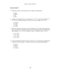
and the total entropy would be maximized when dS would be zero for changes dx. Stating thatdS tot = 0 is equivalent to stating that dF a = 0 at fixed T , where F a = E a − T S a is the Helmholtzfree energy of system a,dS tot | T,Q,V = − 1 T dF a| T,Q,V = 0. (1.33)Thus, if a system is in contact with a heat bath at temperature T , the value of x adjusts itselfto minimize (since the entropy comes in with the opposite sign) F (x, T, V, Q). If charges are alsoallowed to enter/exit the system with a bath at chemical potential µ, the change in entropy isHere, stating that dS tot = 0 is equivalent to stating,dS tot = dS a − dE a /T + µ a dQ a /T = 0. (1.34)dS tot | T,V,µ = d(S a − βE a + βµQ a )| T,V,µ = d P VT∣ = 0, (1.35)T,V,µThus, at fixed chemical potential and temperature a system adjusts itself to maximize the pressure.The calculations above assumed that the volume was fixed. In some instances, the pressure andparticle number might be fixed rather than the chemical potential and volume. In that case,This can then be stated as:dS tot = dS a − dE a /T − βP dV a = 0. (1.36)d(S a − βE a − βP V a ) | T,Q,P = −βd(µQ) = 0. (1.37)Here, the term µQ is referred to as the Gibb’s free energy,Summarizing the four cases discussed above:G ≡ µQ = E + P V − T S. (1.38)• If E, V and Q are fixed, x is chosen to maximize S(x, E, V, Q).• If Q and V are fixed, and the system is connected to a heat bath, x is chosen to minimizeF (x, T, V, Q).• If the system is allowed to exchange charge and energy with a bath at chemical potential µand temperature T , x is chosen to maximize P (x, T, µ, V ) (or Ω GC in the case that there arelong range correlations or interactions).• If the charge is fixed, but the volume is allowed to adjust itself at fixed pressure, the systemwill attempt to minimize the Gibb’s free energy, G(x, T, P, Q).Perhaps the most famous calculation of this type concerns the electroweak phase transition whichpurportedly took place in the very early universe, 10 −12 s after the big bang. In that transition theHigg’s condensate ⟨ϕ⟩ became non-zero in a process called spontaneous symmetry breaking. Thefree energy can be calculated as a function of ⟨ϕ⟩ (Search literature of 1970s by Jackiw, Colemanand Linde). The resulting free energy depends on T and ⟨ϕ⟩, as illustrated qualitatively in Fig. 1.1.9

Figure 1.1: The free energy has a minimum at nonzero⟨ϕ⟩ at T = 0. In such circumstances a condensedfield forms, as is the case for the Higg’s condensate forthe electroweak transition or the scalar quark condensatefor the QCD chiral transition. At high temperature, theminimum moves back to ⟨ϕ⟩ = 0. If ⟨ϕ⟩ is discontinuousas a function of T , a phase transition ensues. If ⟨ϕ⟩ is multidimensional, i.e., ϕ has two components with rotationalsymmetry, the transition violates symmetry and isreferred to a spontaneous symmetry breaking. Such potentialsare often referred to as “mexican hat” potentials.1.8 Free EnergiesPerusing the literature, one is likely to find mention of several free energies. For macroscopic systemswithout long-range interactions one can write the grand potential as P V . The other common freeenergies can also be expressed in terms of the pressure as listed below:Grand Potential Ω = P V = T S − E + µQHelmholtz Free Energy F = E − T S = µQ − P VGibb’s Free Energy G = µQ = E + P V − T SEnthalpy ∗ H = E + P V = T S + µQTable 2: Various free energies∗ Enthalpy is conserved in what is called a Joule-Thomson process, see http://en.wikipedia.org/wiki/Joule-Thomson effect#Proof that enthalpy remains constant in a Joule-Thomson process.In the grand canonical ensemble, one finds the quantities E and Q by taking derivatives of thegrand potential w.r.t. the Lagrange multipliers. Similarly, one can find the Lagrange multipliers bytaking derivatives of some of the other free energies with respect to Q or E. To see this we beginwith the fundamental thermodynamic relation,T dS = dE + P dV − µdQ. (1.39)Since the Helmholtz free energy is usually calculated in the canonical ensemble,F = −T ln Z C (Q, T, V ) = E − T S, (1.40)it is typically given as a function of Q and T . Nonetheless, one can still find µ by considering,dF = dE − T dS − SdT = −P dV − SdT + µdQ. (1.41)This shows that the chemical potential isµ = ∂F∂N ∣ . (1.42)V,T10

Similarly, in the microcanonical ensemble one typically calculates the entropy as a function ofE and Q. In this case the relationdS = βdE + βP dV − βµdQ, (1.43)allows one to read off the temperature asβ = ∂S∂E ∣ . (1.44)V,NIn many text books, thermodynamics begins from this perspective. We have instead begun with theentropy defined as − ∑ p i ln p i , as this approach does not require the continuum limit, and allows thethermodynamic relations to be generated from general statistical concepts. The question “Whenis statistical mechanics thermodynamics?” is not easily answered. A more meaningful questionconcerns the validity of the fundamental thermodynamic relation, T dS = dE + P dV − µdQ. Thisbecomes valid as long as one can justify differentials, which is always the case for grand canonicalensemble, where E and Q are averages. However, for the other ensembles one must be careful thatthe discreteness of particle number or energy levels invalidates the use of differentials, which is nevera problem for macroscopic systems.1.9 Forces at Finite TemperatureLet’s assume a particle feels a force dependent on it’s position r, but that the force depends on howthe thermal medium reacts to the particle’s position. Normally, one would consider the force fromthe gradient of the energy, F i = −∂ i E(r). Indeed, this is the case in a thermal system,F i = − ∂E(r)∂r i∣ ∣∣∣S,where the partial derivative is taken at constant entropy. This is based on the idea that the particlemoves slowly, and that the particle remains in the a given, but shifting, energy level of the systemas the coordinate is slowly varied.However, thermal calculations are often performed more readily at fixed temperature, ratherthan fixed entropy. For that reason, one would like to know how to calculate the force usingderivatives where the temperature is fixed, and then correct for the fact that the temperature mustbe altered to maintain constant entropy. For simplicity, consider a one-dimensional system.δE = ∂E∂x ∣ δx + ∂ET∂T ∣ δT, (1.45)xδS = 0 = ∂S∂x ∣ δx + ∂ST∂T ∣ δT.xNow, solve for δT in the lower expression and substitute into the upper expression to obtain,δE| S= ∂E∂x ∣ δx − ∂ T E∂ x Sδx (1.46)T∂ T S{ ∂E= δx∂x ∣ − T ∂S}T∂x ∣ ,T11

where the last step made use of the definition of temperature from Eq. (1.44),∂ T E∂ T S= dE/dS = T. (1.47)So, by inspection of Eq. (1.46) the force can now be state as∂E∂(E − T S)∂x ∣ = S∂x ∣ , (1.48)Tand the Helmholtz free energy, F = E − T S, plays the role of the potential. This result should notbe interpreted as the particle feels a force that pushes it towards minimizing the potential energyand maximizing the entropy. Particles don’t feel entropy. The −T S term comes from having takengradients at fixed temperature, whereas the definition of the force is the derivative of the potentialenergy with respect to x at fixed entropy.1.10 Maxwell RelationsMaxwell relations are a set of equivalences between derivatives of thermodynamic variables. Theycan prove useful in several cases, for example in the Clausius-Claeyron equation, which will bediscussed later. Derivations of Maxwell relations also tends to appear in written examinations.All Maxwell relations can be derived from the fundamental thermodynamic relation,dS = βdE + (βP )dV − (βµ)dQ, (1.49)from which one can readily identify β, P and µ with partial derivatives,β = ∂S∂E ∣ , (1.50)V,QβP = ∂S∂V ∣ ,E,Qβµ = − ∂S∂Q∣ .E,VHere, the subscripts refer to the quantities that are fixed. Since for any continuous function f(x, y),∂ 2 f/(∂x∂y) = ∂ 2 f/(∂y∂x), one can state the following identities which are known as Maxwellrelations,∂β∂V ∣ = ∂(βP )E,Q∂E ∣ , (1.51)V,Q∂β∂Q∣ = − ∂(βµ)E,V∂E ∣ ,V,Q∂(βP )∂Q ∣ = − ∂(βµ)β,V∂V ∣ .β,QAn entirely different set of relations can be derived by beginning with quantities other than dS.For instance, if one begins with dF ,F = E − T S, (1.52)dF = dE − SdT − T dS,= −SdT − P dV − µdQ,12

three more Maxwell relations can be derived by considering second derivatives of F with respect toT, V and Q. Other sets can be derived by considering the Gibbs free energy, G = E + P V − T S,or the pressure, P V = T S − E + µQ.EXAMPLE:Validate the following Maxwell relation:Start with the standard relation,∂V∂Q∣ = ∂µP,T∂P ∣ (1.53)T,QdS = βdE + (βP )dV − (βµ)dQ. (1.54)This will yield Maxwell’s relations where E, V and Q are held constant. Since we want a relationwhere T, N and P/T are held constant, we should consider:This allows one to realize:V = −d(S − (βP )V − βE) = −Edβ − V d(βP ) − (βµ)dQ. (1.55)∂(S − βP V − βE)∂(βP )∣ ,β,Qβµ = −∂(S − βP V − βE)∂Q∣ . (1.56)β,βPUsing the fact that ∂ 2 f/(∂x∂y) = ∂ 2 f/(∂y∂x),∂V∂Q∣ = ∂βµβP,T∂βP ∣ . (1.57)β,QOn the l.h.s., fixing βP is equivalent to fixing P since T is also fixed. On the r.h.s., the factors ofβ in ∂(βµ)/∂(βP ) cancel because T is fixed. This then leads to the desired result, Eq. (1.53).ANOTHER EXAMPLE:Show that∂E∂Q∣ = µ − P ∂µ∣S,P∂POne way to start is to look at the relation and realize that V does not appear. Thus, let’s rewritethe fundamental thermodynamic relation with dV = · · · . This ensures that we won’t have any V sappearing on the r.h.s. of the equations going forward.∣S,QdV = T P dS − 1 P dE + µ P dQ.Now, since the relation will involve S, P and Q being constant add d(E/P ) from each side to getd(V + E/P ) = T P dS + Ed(1/P ) + µ P dQ∂E∂Q∣ = ∂(µ/P )S,P∂(1/P ) ∣S,Q= µ − P ∂µ∣∂P13∣S,Q

Some students find a nmemonic useful for deriving some of the Maxwell relations. Seehttp://en.wikipedia.org/wiki/Thermodynamic square. However, this is more cute than useful. Asyou will see with some of the more difficult problems at the end of this chapter.1.11 FluctuationsStatistical averages of higher order terms in the energy or the density can also be extracted from thepartition function. For instance, in the grand canonical ensemble (using β = 1/T and α = −µ/Tas the variables),∂ 2 β ln Z(β, α) = ∂ β∂ β ZZ= 1 Z ∂2 βZ −( 1Z ∂ βZ) 2(1.58)= ⟨ E 2 ⟩ − ⟨E ⟩ 2= ⟨ (E − ⟨E⟩) 2⟩ .Thus, the second derivative of ln Z gives the fluctuation of the energy from its average value.Similarly, one can see that∂ β ∂ α ln Z = ⟨(E − ⟨E⟩)(Q − ⟨Q⟩)⟩ (1.59)∂ β ∂ α ln Z = ⟨ (Q − ⟨Q⟩) 2⟩ . (1.60)Fluctuations play a critical role in numerous areas of physics, most notably in critical phenomena.1.12 Problems1. Using the methods of Lagrange multipliers, find x and y that minimize the following function,f(x, y) = 3x 2 − 4xy + y 2 ,subject to the constraint,3x + y = 0.2. Consider 2 identical bosons (A given level can have an arbitrary number of particles) in a2-level system, where the energies are 0 and ϵ. In terms of ϵ and the temperature T , calculate:(a) The partition function Z C(b) The average energy ⟨E⟩. Also, give ⟨E⟩ in the T = 0, ∞ limits.(c) The entropy S. Also give S in the T = 0, ∞ limits.(d) Now, connect the system to a particle bath with chemical potential µ. Calculate Z GC (µ, T ).Find the average number of particles, ⟨N⟩ as a function of µ and T . Also, give theT = 0, ∞ limits.Hint: For a grand-canonical partition function of non-interacting particles, one can state14

that Z GC = Z 1 Z 2 · · · Z n , where Z i is the partition function for one single-particle level,Z i = 1+e −β(ϵ i−µ) +e −2β(ϵ i−µ) +e −3β(ϵ i−µ) · · · , where each term refers to a specific numberof bosons in that level.3. Repeat the problem above assuming the particles are identical Fermions (No level can havemore than one particle, e.g., both are spin-up electrons).4. Beginning with the expression,T dS = dE + P dV − µdQ,show that the pressure can be derived from the Helmholtz free energy, F = E − T S, withP = − ∂F∂V ∣ .Q,T5. Beginning with:derive the Maxwell relation,dE = T dS − P dV + µdQ,∂V∂µ ∣ = − ∂NS,P∂P ∣ .S,µ6. Assuming that the pressure P is independent of V when written as a function of µ and T ,i.e., ln Z GC = P V/T (true if the system is much larger than the range of interaction),(a) Find expressions for E/V and Q/V in terms of P/T , and partial derivatives of P/Tw.r.t. α ≡ −µ/T and β ≡ 1/T . Here, assume the chemical potential is associated withthe conserved number Q.(b) Find an expression for C V = dE/dT | N,V in terms of P/T , E, Q, V and the derivativesof P/T , E and Q w.r.t. β and α.7. Beginning with the definition,Show that∂C p∂PC P = T ∂S∂T∣ ,N,P∣ ∣ = −T ∂2 V ∣∣∣P,NT,N∂T 2Hint: Find a quantity Y for which both sides of the equation become ∂ 3 Y/∂ 2 T ∂P .8. Beginning withT dS = dE + P dV − µdQ, and G ≡ E + P V − T S,(a) Show thatS = − ∂G∂T∣ ,N,PV = ∂G∂P∣ .N,T15

(b) Beginning withδS(P, N, T ) = ∂S ∂S ∂SδP + δN +∂P ∂N ∂T δT,Show that the specific heats,C P ≡ T ∂S∂T ∣ , C V ≡ T ∂SN,P∂T ∣ ,N,Vsatisfy the relation:C P = C V − T(∂V∂T) 2 (∣P,N∂V∂P) −1∣T,NNote that the compressibility, ≡ −∂V/∂P , is positive (unless the system is unstable),therefore C P > C V .9. From Sec. 1.11, it was shown how to derive fluctuations in the grand canonical ensemble.Thus, it is straightforward to find expressions for the following fluctuations, ϕ EE ≡⟨δEδE⟩/V, ϕ QQ ≡ ⟨δQδQ⟩/V and ϕ QE ≡ ⟨δEδQ⟩/V . In terms of the 3 fluctuations calculatedin the grand canonical ensemble, and in terms of the volume and the temperature T ,express the specific heat at constant volume,C V = dEdT∣ .Q,VNote that the fluctuation observables, ϕ ij , are intrinsic quantities, assuming that the correlationsin energy density occur within a finite range and that the overall volume is much largerthan that range.16

2 Statistical Mechanics of Non-Interacting Particles“Its a gas! gas! gas!” - M. Jagger & K. RichardsWhen students think of gases, they usually think back to high school physics or chemistry, andthink of the ideal gas law. This simple physics applies for gases which are sufficiently dilute thatinteractions between particles can be neglected and that identical-particle statistics can be ignored.For this chapter, we will indeed confine ourselves to the assumption that interactions can be neglected,but will consider in detail the effects of quantum statistics. Quantum statistics play adominant role in situations across all fields of physics. For instance, Fermi gas concepts play theessential role in understanding nuclear structure, stellar structure and dynamics, and the propertiesof metals and superconductors. For Bose systems, quantum degeneracy plays the central role inliquid Helium and in many atom/molecule trap systems. Even in the presence of strong interactionsbetween constituents, the role of quantum degeneracy still plays the dominant role in determiningthe properties and behaviors of numerous systems.2.1 Non-Interacting GasesA non-interacting gas can be considered as a set of independent momentum modes, labeled by themomentum p. For particles in a box defined by 0 < x < L x , 0 < y < L y , 0 < z < L z , the wavefunctions have the form,ψ px ,p y ,p z(x, y, z) ∼ sin(p x x/¯h) sin(p y y/¯h) sin(p z z/¯h) (2.1)with the quantized momentum ⃗p satisfying the boundary conditions,p x L x /¯h = n x π, n x = 1, 2, · · · , (2.2)p y L y /¯h = n y π, n y = 1, 2, · · · ,p z L z /¯h = n z π, n z = 1, 2, · · ·The number of states in d 3 p is dN = V d 3 p/(π¯h) 3 . Here p x , p y and p z are positive numbers asthe momenta are labels of the static wavefunctions, each of which can be considered as a coherentcombination of a forward and a backward moving plane wave. The states above are not eigenstatesof the momentum operator, as sin px/¯h is a mixture of left-going and right-going states. If one wishesto consider plane waves, the signs of the momenta can be either positive or negative. Since onedoubles the range of momentum for each dimension when one includes both positive and negativemomenta, one needs to introduce a factor of 1/2 to the density of states for each dimension whenincluding the negative momentum states. The density of states in three dimensions then becomes:dN = Vd3 p(2π¯h) 3 . (2.3)For one or two dimensions, d 3 p is replaced by d D p and (2π¯h) 3 is replaced by (2π¯h) D , where D isthe number of dimensions. For two dimensions, the volume is replaced by the area, and in onedimension, the length plays that role.In the grand canonical ensemble, each momentum mode can be considered as being an independentsystem, and being described by its own partition function, z p . Thus, the partition function of17

the entire system is the product of partition functions of each mode,Z GC = ∏ pz p , z p = ∑ n pe −n pβ(ϵ p −µq) . (2.4)Here n p is the number of particles of charge q in the mode, and n p can be 0 or 1 for Fermions, or canbe 0, 1, 2, · · · for bosons. The classical limit corresponds to the case where the probability of havingmore than 1 particle would be so small that the Fermi and Bose cases become indistinguishable.Later on it will be shown that this limit requires that µ is much smaller (in units of T ) than theenergy of the lowest mode.For thermodynamic quantities, only ln Z GC plays a role, which allows the product in Eq. (2.4)to be replaced by a sum,ln Z GC = ∑ ln z p (2.5)p∫ V d 3 p= (2s + 1)(2π¯h) ln z 3 p∫ V d 3 p= (2s + 1)(2π¯h) ln(1 + 3 e−β(ϵ−µq) ) (Fermions),∫ ()V d 3 p= (2s + 1)(2π¯h) ln 1(Bosons).3 1 − e −β(ϵ−µq)Here, the intrinsic spin of the particles is s. For the Fermi expression, where z p = 1 + e −β(ϵp−µ) ,the first term represents the contribution for having zero particles in the state and the second termaccounts for having one particle in the level. For bosons, which need not obey the Pauli exclusionprinciple, one would include additional terms for having 2, 3 · · · particles in the mode, and theBosonic relation has made use of the fact that 1 + x + x 2 + x 3 · · · = 1/(1 − x).EXAMPLE:For a classical two-dimensional, non-interacting, non-relativistic gas of fermions of mass m, andcharge q = 1 and spin s, find the charge density and energy density of a gas in terms of µ and T .The charge can be found by taking derivatives of ln Z GC with respect to µ,Q =∂∂(βµ) ln Z GC, (2.6)= (2s + 1)A∫ ∞02πp dp(2π¯h) · e −β(p2 /2m−µ)2 1 + e −β(p2 /2m−µ)= (2s + 1)A mT ∫ ∞2π¯h 2 dxe−(x−βµ)1 + e . −(x−βµ)The above expression applies to Fermions. To apply the classical limit, one takes the limit that theβµ → −∞,QA0∫mT ∞= (2s + 1)2π¯h 2 dx e −(x−βµ) (2.7)0= (2s + 1) mT2π¯h 2 eβµ .18

In calculating the energy per unit area, one follows a similar procedure beginning with,E = − ∂∂β ln Z GC, (2.8)∫E∞A = (2s + 1)02πp dp p 2(2π¯h) 2 2me −β(p2 /2m−µ)1 + e −β(p2 /2m−µq)= (2s + 1) mT 2 ∫ ∞2π¯h 2 dx xe−(x−βµ)1 + e −(x−βµ)≈ (2s + 1) mT 202π¯h 2 eβµ , (2.9)where in the last step we have taken the classical limit. If we had begun with the Bosonic expression,we would have came up with the same answer after assuming βµ → −∞.As can be seen in working the last example, the energy and charge can be determined by thefollowing integrals,∫= (2s + 1)QVEV∫= (2s + 1)d D pf(ϵ), (2.10)(2π¯h)Dd D p(2π¯h) D ϵ(p)f(ϵ),where D is again the number of dimensions and f(p) is the occupation probability, a.k.a. thephase-space occupancy or the phase-space filling factor,⎧⎨ e −β(ϵ−µ) /(1 + e −β(ϵ−µ) ), Fermions, Fermi − Dirac distributionf(ϵ) = e −β(ϵ−µ) /(1 − e −β(ϵ−µ) ), Bosons, Bose − Einstein distribution (2.11)⎩e −β(ϵ−µ) , Classical, Boltzmann distribution.Here f(ϵ) can be identified as the average number of particles in mode p. These expressions arevalid for both relativistic or non-relativisitc gases, the only difference being that for relativistic gasesϵ(p) = √ m 2 + p 2 .The classical limit is valid whenever the occupancies are always much less than unity, i.e.,e β(µ−ϵ0) ≪ 1, or equivalently β(µ−ϵ 0 ) → −∞. Here, ϵ 0 refers to the energy of the lowest momentummode, which is zero for a massless gas, or for a non-relativistic gas where the rest-mass energy isignored, ϵ = p 2 /2m. If one preserves the rest-mass energy in ϵ(p), then ϵ 0 = mc 2 . The decision toignore the rest-mass in ϵ(p) is accompanied by translating µ by the same amount. For relativisticsystems, one usually keeps the rest mass energy because one can not ignore the contribution fromanti-particles. For instance, if one has a gas of electrons and positrons, the chemical potentialmodifies the phase space occupancy through a factor e βµ , while the anti-particle is affected by e −βµ ,and absorbing the rest-mass into µ would destroy the symmetry between the expressions for thedensities of particles and anti-particles.2.2 Equi-partition and Virial TheoremsParticles undergoing interaction with an external field, as opposed to with each other, also behaveindependently. The phase space expressions from the previous section are again important here,19

as long as the external potential does not confine the particles to such small volumes that theuncertainty principle plays a role. The structure of the individual quantum levels will becomeimportant only if the energy spacing is not much smaller than the temperature.The equi-partition theorem applies for the specific case where the quantum statistics can beneglected, i.e. f(ϵ) = e −β(ϵ−µ) , and one of the variables, p or q, contributes to the energy quadratically.The equi-partition theory states that the average energy associated with that variable is then(1/2)T . This is the case for the momentum of non-relativistic particles being acted on by potentialsdepending only on the position. In that case,E = p2 x + p 2 y + p 2 z2m+ V (r). (2.12)When calculating the average of p 2 x/2m (in the classical limit),⟨ ⟩ ∫ p2x= (2π¯h)−3 dp x dp y dp z d 3 r (p 2 x/2m)e −(p2 x +p2 y +p2 z )/2mT −V (r)/T2m (2π¯h) ∫ , (2.13)−3 dp x dp y dp z d 3 r e −(p2 x+p 2 y+p 2 z)/2mT −V (r)/Tthe integrals over p y , p z and r factorize and then cancel leaving only,⟨ ⟩ p2x=2m∫dpx (p 2 x/2m)e −p2 x/2mT∫dpx e −p2 x /2mT = T 2 . (2.14)The average energy associated with p x is then independent of m.The same would hold for any other degree of freedom that appears in the Hamiltonian quadratically.For instance, if a particle moves in a three-dimensional harmonic oscillator,the average energy isH = p2 x + p 2 y + p 2 z2m+ 1 2 mω2 xx 2 + 1 2 mω2 yy 2 + 1 2 mω2 zz 2 , (2.15)⟨H⟩ = 3T, (2.16)with each of the six degrees of freedom contributing T/2.The generalized equi-partition theorem works for any variable that is confined to a finite region,and states ⟨q ∂H ⟩= T. (2.17)∂qFor the case where the potential is quadratic, this merely states the ungeneralized form of theequi-partition theorem. To prove the generalized form, one need only integrate by parts,⟨q ∂H ⟩ ∫dq q(∂H/∂q) e−βH(q)= ∫ (2.18)∂qdq e−βH(q)= −T ∫ dq q(∂/∂q) e∫ −βH(q)dq e−βH(q)T[qe −βH(q)∣ ∣ ∞ + ∫ ]dq e −βH(q) −∞=∫dq e−βH(q)= T if H(q → ±∞) = ∞.20

Note that disposing of the term with the limits ±∞ requires that H(q → ±∞) → ∞, or equivalently,that the particle is confined to a finite region of phase space. The rule also works if p takes theplace of q.The virial theorem has an analog in classical mechanics, and is often referred to as the “ClausiusVirial Theorem”. It states, ⟨ ⟩ ⟨ ⟩∂H ∂Hp i = q i . (2.19)∂p i ∂q iTo prove the theorem we use Hamilton’s equations of motion,⟨ ddt (q ip i )⟩= ⟨p i ˙q i ⟩ + ⟨q i ṗ i ⟩ =⟨ ⟩∂Hp i −∂p i⟨ ⟩∂Hq i . (2.20)∂q iThe theorem will be proved if the time average of d/dt(p i q i ) = 0. Defining the time average as theaverage over an infinite interval τ,⟨ ddt (p iq i )⟩≡ 1 ∫ τdt d τ dt (p iq i ) = 1 τ (p iq i )| τ 0 , (2.21)0which will equal zero since τ → ∞ and p i q i is finite. Again, this finite-ness requires that theHamiltonian confines both p i and q i to a finite region in phase space. In the first line of theexpression above, the equivalence between the statistical average and the time-weighted averagerequired the the Ergodic theorem.EXAMPLE:Using the virial theorem and the non-generalized equi-partition theorem, show that for a nonrelativisticparticle moving in a one-dimensional potential,that the average potential energy isV (x) = κx 6 ,⟨V (x)⟩ = T/6.To proceed, we first apply the virial theorem to relate an average of the potential to an averageof the kinetic energy which is quadratic in p and can thus be calculated with the equi-partitiontheorem, ⟨x ∂V ⟩ ⟨= p ∂H ⟩=∂x ∂p⟨ ⟩ p2Next, one can identify ⟨x ∂V ⟩= 6 ⟨V (x)⟩ ,∂xto see thatm⟨V (x)⟩ = T 6 .⟨ ⟩ p2= 2 = T. (2.22)2mOne could have obtained this result in one step with the generalized equi-partition theorem.21

2.3 Degenerate Bose GasesThe term degenerate refers to the fact there are some modes for which the occupation probabilityf(p) is not much smaller than unity. In such cases, Fermions and Bosons behave very differently.For bosons, the occupation probability,f(ϵ) =e−β(ϵ−µ), (2.23)1 − e−β(ϵ−µ) will diverge if µ reaches ϵ. For the non-relativistic case (ϵ = p 2 /2m ignoring the rest-mass energy)this means that a divergence will ensue if µ ≥ 0. For the relativistic case (ϵ = √ p 2 + m 2 includesthe rest-mass in the energy) a divergence will ensue when µ ≥ m. This divergence leads to thephenomena of Bose condensation.To find the density required for Bose condensation, one needs to calculate the density for µ → 0 − .For lower densities, µ will be negative and there are no singularities in the phase space density. Thecalculation is a bit tedious but straight-forward,∫ρ(µ = 0 − , T ) = (2s + 1)∫= (2s + 1)d D p(2π¯h) Dd D p(2π¯h) De −p2 /2mT1 − e −p2 /2mT∞∑n=1(∫(mT )D/2= (2s + 1)(2π¯h) De −np2 /2mT ,)∑ ∞d D xe −x2 /2n=1n −D/2(2.24)For D = 1, 2, the sum over n diverges. Thus for one or two dimensions, Bose condensation neveroccurs (at least for massive particles where ϵ p ∼ p 2 ) as one can attain an arbitrarily high densitywithout having µ reach zero. This can also be seen by expanding f(ϵ) for ϵ p and µ near zero,f(p → 0) ≈1βp 2 /m − βµ . (2.25)For D = 1, 2, the phase space weight p D−1 dp will not kill the divergence of f(p → 0) in the limitµ → 0. Thus, one can obtain arbitrarily high densities without µ actually reaching 0. Since µ neverreaches zero, even as the density approaches infinite, Bose condensation never occurs.For D = 3, the condensation density is finite,(∫(mT )3/2ρ(µ = 0) = (2s + 1)(2π¯h) 3where ζ(n) is the Riemann-Zeta function,(mT )3/2= (2s + 1)3ζ(3/2),(2π)3/2¯h)∑ ∞d 3 xe −x2 /2n=1n −3/2 (2.26)ζ(n) ≡∞∑j=11j n (2.27)22

The Riemann-Zeta function appears often in statistical mechanics, and especially often in graduatewritten exams. Some values are:ζ(3/2) = 2.612375348685... ζ(2) = π 2 /6, ζ(3) = 1.202056903150..., ζ(4) = π 4 /90 (2.28)Once the density exceeds ρ c = ρ(µ = 0), µ no longer continues to rise. Instead, the occupationprobability of the ground state,f =e−β(ϵ 0−µ)1 − e , (2.29)−β(ϵ 0−µ)becomes undefined, and any additional density above ρ c is carried by particles in the ground state.The gas has two components. For the normal component, the momentum distribution is describedby the normal Bose-Einstein distribution with µ = 0 and has a density of ρ c , while the condensationcomponent has density ρ − ρ c . Similarly, one can fix the density and find the critical temperatureT c , below which the system condenses.Having a finite fraction of the particles in the ground state does not explain superfluidity byitself. However, particles at very small relative momentum (in this case zero) will naturally formordered systems if given some kind of interaction (For dilute gases the interaction must be repulsive,as otherwise the particles would form droplets). An ordered conglomeration of bosons will also movewith remarkably little friction. This is due to the fact that a “gap” energy is required to removeany of the particles from the ordered system, thus allowing the macroscopic condensate to movecoherently as a single object carrying a macroscopic amount of current even though it moves veryslowly. Since particles bounce elastically off the condensate, the drag force is proportional to thesquare of the velocity (just like the drag force on a car moving through air) and is negligible fora slow moving condensate. Before the innovations in atom traps during the last 15 years, theonly known Bose condensate was liquid Helium-4, which condenses at atmospheric pressure at atemperature of 2.17 ◦ K, called the lambda point. Even though liquid Helium-4 is made of tightlypacked, and therefore strongly interacting, atoms, the prediction for the critical temperature usingthe calculations above is only off by a degree or so.EXAMPLE:Photons are bosons and have no charge, thus no chemical potential. Find the energy density andpressure of a two-dimensional gas of photons (ϵ = p) as a function of the temperature T . Note:whereas in three dimensions photons have two polarizations, they would have only one polarizationin two dimensions. Also, in two dimensions the pressure is a force per unity length, not a force perunit area as it is in three dimensions.First, write down an expression for the pressure (See HW problem),∫1P = 2πpdp p2 e −ϵ/T, (2.30)(2π¯h) 2 2ϵ 1 − e−ϵ/T which after replacing ϵ = p,P =∫14π¯h 2= T 34π¯h 2 ∫e−p/Tp 2 dp . (2.31)1 − e−p/T x 2 dx { e −x + e −2x + e −3x + · · · } ,= T {32π¯h 2 1 + 1 2 + 1 }3 3 + · · · = T 33 2π¯h 2 ζ(3),23

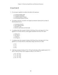
where the Riemann-Zeta function, ζ(3), is 1.202056903150... Finally, the energy density, by inspectionof the expression for the pressure, is E/V = 2P .2.4 Degenerate Fermi GasesAt zero temperature, the Fermi-Dirac distribution becomes,f(T → 0) =e−β(ϵ−µ)1 + e −β(ϵ−µ) ∣∣∣∣β→∞= Θ(µ − ϵ), (2.32)a step-function, which is unity for energies below the chemical potential and zero for ϵ > µ. Thedensity is then,ρ(µ, T = 0) =For three dimensions, the density of states is:D(ϵ)/V =∫ µ0dϵ D(ϵ)/V (2.33)(2s + 1)(2π¯h) 3 (4πp2 ) dpdϵ . (2.34)For small temperatures (much smaller than µ) one can expand f in the neighborhood of µ,f(ϵ) = f 0 + δf, (2.35){ e−ϵ ′δf =/T /(1 + e −ϵ′ /T ) − 1, ϵ ′ ≡ ϵ − µ < 0e −ϵ′ /T /(1 + e −ϵ′ /T ), ϵ ′ > 0{ −eϵ ′=/T /(1 + e ϵ′ /T ), ϵ ′ < 0e −ϵ′ /T /(1 + e −ϵ′ /T ), ϵ ′ .> 0The function δf is illustrated in Fig. 2.1. The function δf(ϵ ′ ) is ∓1/2 at ϵ ′ = 0 and returns to zerofor |ϵ ′ | >> T . Also, δf is an odd function in ϵ ′ , which will be important below.One can expand D(µ + ϵ ′ ) in powers of ϵ ′ , and if the temperature is small, one need only keepthe first term in the Taylor expansion if one is considering the limit of small temperature.ρ(µ, T ) ≈ ρ(µ, T = 0) + 1 ∫ ∞[dϵ ′ D(µ) + ϵ ′ dD ]δf(ϵ ′ ), (2.36)V −∞dϵE≈E V V (µ, T = 0) + 1 ∫ ∞[dϵ ′ (µ + ϵ ′ ) D(µ) + ϵ ′ dD ]δf(ϵ ′ ).Vdϵ−∞Since one integrates from −∞ → ∞, one need only keep terms in the integrand which are even inϵ ′ . Given that δf is odd in ϵ ′ , the following terms remain,δρ(µ, T ) = 2 dDI(T ), (2.37)( ) V dϵEδ = µδρ + 2 D(µ)I(T ), (2.38)V VI(T )∫ ∞≡ dϵ ′ ϵ ′ e −ϵ′ /T0 1 + e −ϵ′ /T∫ ∞= T 2 dx xe−x1 + e . −x024

10.5f(ε)0.5δ f(ε)0ε'00µε-0.50εFigure 2.1: The phase space density at small temperature is shown in red, while the phase space densityat zero temperature is shown in green.With some trickery, I(T ) can be written in terms of ζ(2),∫ ∞I(T ) = T 2 dx x ( e −x − e −2x + e 3x − e −4x + · · · ) , (2.39)0∫ ∞= T 2 dx x {( e −x + e −2x + e 3x + · · · ) − 2 ( e −2x + e −4x + e 6x + e −8x + · · · )} ,0= T 2 ζ(2) − 2(T/2) 2 ζ(2) = T 2 ζ(2)/2,where ζ(2) = π 2 /6. This gives the final expressions:δρ(µ, T ) = π2 T 2( ) EδV6VdDdϵ∣ , (2.40)ϵ=µ= µδρ + π2 T 2D(µ). (2.41)6VThese expressions are true for any number of dimensions, as the dimensionality affects the answerby changing the values of D and dD/dϵ. Both expressions assume that µ is fixed. If ρ if fixedinstead, the µδρ term in the expression for δE is neglected. It is remarkable to note that theexcitation energy rises as the square of the temperature for any number of dimensions. One powerof the temperature can be thought of as characterizing the range of energies δϵ, over which theFermi distribution is affected, while the second power comes from the change of energy associatedwith moving a particle from µ − δϵ to µ + δϵ.EXAMPLE:Find the specific heat for a relativistic three-dimensional gas of Fermions of mass m, spin s anddensity ρ at low temperature T .Even though the temperature is small, the system can still be relativistic if µ is not muchsmaller than the rest mass. Such is the case for the electron gas inside a neutron star. In that case,25

ϵ = √ m 2 + p 2 which leads to dϵ/dp = p/ϵ, and the density of states and the derivative from Eq.(2.34) becomes(2s + 1)D(ϵ) = V 4πpϵ . (2.42)(2π¯h)3The excitation energy is then:δE fixed N = (2S + 1) p fϵ f V12¯h 3 T 2 , (2.43)where p f and ϵ f are the Fermi momentum and Fermi energy, i.e., the momentum where ϵ(p f ) =ϵ f = µ at zero temperature. For the specific heat this yields:C V = dE/dTρV= (2S + 1) 2p fϵ f12¯h 3 T. (2.44)ρTo express the answer in terms of the density, one can use the fact that at zero temperature,ρ =(2s + 1) 4πp 3 f(2π¯h) 3 3 , (2.45)to substitute for p f in the expression for C V .One final note: Rather than using the chemical potential or the density, author’s often referto the Fermi energy ϵ f , the Fermi momentum p f , or the Fermi wave-number k f = p f /¯h. Thesequantities usually refer to the density, rather than to the chemical potential, though not necessarilyalways. That is, since the chemical potential changes as the temperature rises from zero to maintaina fixed density, it is somewhat arbitrary as to whether ϵ f refers to the chemical potential, or whetherit refers to the chemical potential one would have used if T were zero. Usually, the latter criteriumis used for defining ϵ f , p f and k f . Furthermore, ϵ f is always measured relative to the energy forwhich p = 0, whereas µ is measured relative to the total energy which would include the potential.For instance, if there was a gas of density ρ, the Fermi momentum would be defined by:1 4πρ = (2s + 1)(2π¯h) 3 3 p3 f, (2.46)and the Fermi energy (for the non-relativistic case) would be given by:ϵ f = p2 f2m . (2.47)If there were an attractive potential of strength V , the chemical potential at zero temperature wouldthen be ϵ f −V . If the temperature were raised while keeping ρ fixed, p f and ϵ f would keep constant,but µ would change to keep ρ fixed, consistent with Eq. (2.40).ANOTHER EXAMPLE:Consider a two-dimensional non-relativistic gas of spin-1/2 Fermions of mass m at fixed chemicalpotential µ.(A) For a small temperature T , find the change in density to order T 2 .26

(B) In terms of ρ and m, what is the energy per particle at T = 0(C) In terms of ρ, m and T , what is the change in energy per particle to order T 2 .First, calculate the density of states for two dimensions,AD(ϵ) = 2(2π¯h) 2πpdp 2 dϵ =A2m, (2.48)π¯hwhich is independent of p f . Thus, dD/dϵ = 0, and as can be seen from Eq. (2.40), the density doesnot change to order T 2 .The number of particles in area A is:N = 2A 1(2π¯h) 2 πp2 f =and the total energy of those particles at zero temperature is:E = 2A 1(2π¯h) 2 ∫ pf02πp f dp fand the energy per particle becomesEN ∣ = p2 fT =04m = ϵ f2 , p f =From Eq. (2.41), the change in the energy is:and the energy per particle changes by an amount,A2π¯h 2 p2 f, (2.49)p 2 f2m =A8mπ¯h 2 p4 f, (2.50)√2π¯h 2 ρ. (2.51)δE = D(µ) π26 T 2 = A πm6¯h 2 T 2 , (2.52)δEN = πm6¯h 2 ρ T 2 (2.53)2.5 Grand Canonical vs. CanonicalIn the macroscopic limit, the grand canonical ensemble is usually the easiest to work with. However,when working with only a few particles, there are differences between the restriction that only thosestates with exactly N particles are considered, as opposed to the restriction that the average numberis N. This difference can matter when the fluctuation of the number, which usually goes as √ N,is not much less than N itself. To understand how this comes about, consider the grand canonicalpartition function,Z GC (µ, T ) = ∑ e µN/T Z C (N, T ). (2.54)NThermodynamic quantities depend on the log of the partition function. If the contributions to Z GCcome from a range of ¯N ± δN, we can approximate ZGC by,Z GC (µ, T ) ≈ δNe µ ¯N/T Z C ( ¯N, T ) (2.55)ln Z GC ≈ µ ¯N/T + ln Z C ( ¯N, T ) + ln δN,27

and if one calculates the entropy from the two ensembles, ln Z GC +βĒ−µ ¯N/T in the grand canonicalensemble and ln Z + βĒ in the canonical ensemble, one will see that the entropy is greater in thegrand canonical case by an amount,S GC ≈ S C + ln δN. (2.56)The entropy is greater in the grand canonical ensemble because more states are being considered.However, in the limit that the system becomes macroscopic, ln Z C will rise proportional to N,and if one calculates the entropy per particle, S/N, the canonical and grand canonical results willbecome identical. For 100 particles, δN ≈ √ N = 10, and the entropy per particle differs only byln 10/100 ≈ 0.023. As a comparison, the entropy per particle of a gas at room temperature is onthe order of 20 and the entropy of a quantum gas of quarks and gluons at high temperature isapproximately four units per particle.2.6 Gibb’s ParadoxNext, we consider the manifestations of particles being identical in the classical limit, i.e., the limitwhen there is little chance two particles are in the same single-particle level. We consider thepartition function Z C (N, T ) for N identical spinless particles,Z C (N, T ) =z(T )NN!where z(T ) is the partition function of a single particle,, (2.57)z(T ) = ∑ pe −βϵ p. (2.58)In the macroscopic limit, the sum over momentum states can be replaced by an integral, ∑ p →[V/(2π¯h) 3 ] ∫ d 3 p.If the particles were not identical, there would be no 1/N! factor in Eq. (2.57). This factororiginates from the fact that if particle a is in level i and particle b is in level j, there is no differencefrom the state where a is in j and b is in i. This is related to Gibb’s paradox, which concerns theentropy of two gases of non-identical particles separated by a partition. If the partition is lifted, theentropy of each particle, which has a contribution proportional to ln V , will increase by an amountln 2. The total entropy will then increase by N ln V . However, if one states that the particles areidentical and thus includes the 1/N! factor in Eq. (2.57), the change in the total entropy due tothe 1/N! factor is, using Stirling’s approximation,∆S (from 1/N! term) = − ln N! + 2 ln(N/2)! ≈ −N ln 2. (2.59)Here, the first term comes from the 1/N! term in the denominator of Eq. (2.57), and the secondterm comes from the consideration of the same terms for each of the two sub-volumes. Thisexactly cancels the N ln 2 factors inherent to doubling the volume, and the total entropy is notaffected by the removal of the partition. This underscores the importance of taking into accountthe indistinguishability of particles even when there is no significant quantum degeneracy.28

To again demonstrate the effect of the particles being identical, we calculate the entropy for athree-dimensional classical gas of N particles in the canonical ensemble.S = ln Z C + βE = N ln z(T ) − N log(N) + N + βE, (2.60)∫( ) 3/2VmTz(T ) =d 3 p e −p2 /2mT = V(2π¯h) 3 2π¯h 2 , (2.61)[ ( ) ] 3/2V mTS/N = lnN 2π¯h 2 + 5 2 , (2.62)where the equipartition theorem was applied, E/N = 3T/2). The beauty of the expression is thatthe volume of the system does not matter, only V/N, the volume per identical particle. This meansthat when calculating the entropy per particle in a dilute gas, one can calculate the entropy of oneparticle in a volume equal to the subvolume required so that the average number of particles in thevolume is unity. Note that if the components of a gas have spin s, the volume per identical particlewould be (2s + 1)V/N.2.7 Iterative Techniques for the Canonical and Microcanonical EnsemblesThe 1/N! factor must be changed if there is a non-negligible probability for two particles to be inthe same state p. For instance, the factor z N in Eq. (2.57) contains only one contribution for allN particles being in the ground state, so there should be no need to divide that contribution byN! (if the particles are bosons, if they are Fermions one must disregard any contribution with morethan 1 particle per state). To include the degeneracy for a gas of bosons, one can use an iterativeprocedure. First, assume you have correctly calculated the partition function for N − 1 particles.The partition function for N particles can be written as:Z(N) = 1 Nz (n) ≡ ∑ p{z (1) Z(N − 1) ± z (2) Z(N − 2) + z (3) Z(N − 3) ± z (4) Z(N − 4) · · · } , (2.63)e −nβϵ p.Here, the ± signs refer to Bosons/Fermions. If only the first term is considered, one recreates Eq.(2.57) after beginning with Z(N = 0) = 1 (only one way to arrange zero particles). Proof of thisiterative relation can be accomplished by considering the trace of e −βH using symmetrized/antisymmetrizedwave functions (See Pratt, PRL84, p.4255, 2000).If energy and particle number are conserved, one then works with the microcanonical ensemble.Since energy is a continuous variable, constraining the energy is usually somewhat awkward. However,for the harmonic oscillator energy levels are evenly spaced, which allows iterative treatments tobe applied. If the energy levels are 0, ϵ, 2ϵ · · · , the number of ways, N(A, E) to arrange A identicalparticles so that the total energy is E = nϵ can be found by an iterative relation,N(A, E) = 1 AA∑ ∑(±1) a−1 N(A − a, E − aϵ i ), (2.64)a=1 i29

where i de<strong>notes</strong> a specific quantum state. For the Fermionic case this relation can be used to solvea problem considered by Euler, “How many ways can a integers be arranged to sum to E withoutusing the same number twice?”Iterative techniques similar to the ones mentioned here can also incorporate conservation ofmultiple charges, angular momentum, and in the case of QCD, can even include the constraint thatthe overall state is a coherent color singlet (Pratt and Ruppert, PRC68, 024904, 2003).2.8 Enforcing Canonical and Microcanonical Constraints through Integratingover Complex Chemical PotentialsFor systems that are interactive, or for systems where quantum degeneracy plays an important role,grand canonical partition functions are usually easier to calculate. However, knowing the grandcanonical partition function for all imaginary chemical potentials can lead one to the canonicalpartition function. First, consider the grand canonical partition function with an imaginary chemicalpotential, µ/T = iθ,Z GC (µ = iT θ, T ) = ∑ e −βE i+iθQ i. (2.65)iUsing the fact that,one can see that,δ Q,Qi = 1 ∫ 2πdθ e i(Q−Qi)θ , (2.66)2π 0∫1 2πdθ Z GC (µ = iT θ, T )e −iQθ2π 0= ∑ e −βE iδ Q,Qii(2.67)= Z C (Q, T ).A similar expression can be derived for the microcanonical ensemble,12π∫ ∞−∞dz Z C (T = i/z)e −izE = 12π= ∑ i∫ ∞−∞dz ∑ ie iz(ϵ i−E)δ(E − ϵ i ) = ρ(E).(2.68)As stated previously, the density of states plays the role of the partition function in the microcanonicalensemble.2.9 Problems1. Beginning with the expression for the pressure for a non-interacting gas of bosons,P VT= ln Z GC = ∑ ln ( 1 + e −β(ϵp−µ) + e −2β(ϵp−µ) + · · · ) , ∑ ∫V→ (2s + 1)(2π¯h) 3 ppd 3 p,show thatP =(2s + 1)(2π¯h) 3Here, the energy is relativistic, ϵ = √ p 2 + m 2 .∫d 3 p p2f(p), where f =e−β(ϵ−µ)3ϵ301 − e −β(ϵ−µ) .

2. Derive the corresponding expression for Fermions in the previous problem.3. Derive the corresponding expression for Bosons/Fermions in two dimensions in the previousproblem. Note that in two dimension, P describes the work done per expanding by a unitarea, dW = P dA.4. For the two-dimensional problem above, show that P gives the rate at which momentum istransfered per unit length of the boundary of a 2-d confining box. Use simple kinematicconsiderations.5. Consider classical non-relativistic particles acting through a radially symmetric potential,V (r) = V 0 exp(r/λ).Using the equi-partition and virial theorems, show that⟨ rλ V (r) ⟩= 3T.6. Consider a relativistic (ϵ = √ m 2 + p 2 ) particle moving in one dimension,(a) Using the generalized equi-partition theorem, show that⟨ ⟩ p2= T.ϵ(b) Show the same result by explicitly performing the integrals in⟨ ⟩ ∫p2 dp (p 2 /ϵ)e= ∫ −ϵ/T.ϵ dp e−ϵ/THINT: Integrate the numerator by parts.7. Consider a massless three-dimensional gas of bosons with spin degeneracy N s . Assuming zerochemical potential, find the coefficients A and B for the expressions for the pressure andenergy density,( ) EP = AN s T 4 , = BN s T 4V8. Show that if the previous problem is repeated for Fermions that:A F ermions = 7 8 A Bosons,B F ermions = 7 8 B Bosons.9. Consider a three-dimensional solid at low temperature where both the longitudinal and transversesound speeds are given by c s = 3000 m/s. Calculate the ratio of specific heats,C V (due to phonons)C V (due to photons) ,31

where the photon calculation assumes the photons move in a vacuum of the same volume.Note that for sound waves the energy is ϵ = ¯hω = c s¯hk = c s p. For phonons, there are threepolarizations (two transverse and one longitudinal), and since the temperature is low, one canignore the Debye cutoff which excludes high momentum nodes, as their wavelengths are belowthe spacing of the crystal.Data: c = 3.0 × 10 8 m/s, ¯h = 1.05457266 × 10 −34 Js.10. For a one-dimensional non-relativistic gas of spin-1/2 Fermions of mass m, find the change ofthe chemical potential δµ(T, ρ) necessary to maintain a constant density per unity length, ρ,while the temperature is raised from zero to T . Give answer to order T 2 .11. For a two-dimensional gas of spin-1/2 non-relativistic Fermions of mass m at low temperature,find both the quantities below:d(E/A)d(E/A)dT ∣ ,∣µ,VdTGive both answers to the lowest non-zero order in T , providing the constants of proportionalityin terms of the chemical potential at zero temperature and m.12. Consider harmonic oscillator levels, 0, ϵ, 2ϵ · · · , populated by A Fermions of the same spin.(a) Using the iterative relation in Eq. (2.64) solve for the number of ways, N(A, E), toarrange A particles to a total energy E for all A ≤ 3 and all E ≤ 6ϵ.(b) For N(A = 3, E = 6ϵ), list all the individual ways to arrange the particles.13. Consider a two-dimensional gas of spin-less non-degenerate non-relativistic particles of massm.∣N,V(a) Show that the grand canonical partition function Z GC (µ, T ) is{ }µ/T AmTZ GC (µ, T ) = exp e2π¯h 2(b) Using Eq. (2.67) in Sec. 2.8 and the expression above, show that the canonical partitionfunction Z C (N, T ) is( AmT) N2π¯hZ C (N, T ) =2 N!32

3 Interacting Gases and the Liquid-Gas Phase Transition“yeah my distraction is my defenseagainst this lack of inspirationagainst this slowly deflationyeah the further the horizon you knowthe more it warps my gazethe foreground’s out of focusbut you know I kinda hope it’sjust a phase, just a phasejust a phase, just a phasejust a phase, just a phasejust a phase” - A. Difranco3.1 Virial ExpansionThe virial expansion is defined as an expansion of the pressure in powers of the density,[∞∑( ) ] n−1 ∫ρ (2j + 1)P = ρT A 1 + A n , ρ 0 ≡ d 3 p e −ϵp/T . (3.1)ρ 0 (2π¯h) 3n=2The leading term is always A 1 = 1, as low density matter always behaves as an ideal gas. Thecontribution from interactions to the second order term, A 2 , is negative for attractive interactionsand positive for repulsive interactions. Quantum statistics also affects A 2 . For bosons, the contributionis negative, while for fermions it is positive. The negative contribution for bosons can beunderstood by considering the Bose-Einstein form for the phase-space occupancy, which provides arelatively stronger enhancement to low-momentum particles. This lowers the average momentumof particles colliding with the boundaries, which lowers the pressure relative to P = ρT . Similarly,the contribution is positive for fermions, as the average momentum of a particle in a Fermi gas israised by quantum statistics.Like perturbation theory, virial expansions are only justifiable in the limit that they are unimportant,i.e., either only the first few terms matter. For that reason, the second-order coefficientis often calculated carefully from first principles, but subsequent coefficients are often insertedphenomenologically. The virial expansion will be considered more rigorously in Chapter 6, wherecoefficients will be expressed in terms of phase shifts (only second order) and perturbation theory.3.2 The Van der Waals Eq. of StateAll equations of state, P (ρ, T ), should behave as P = ρT at low density. The second-order virialcoefficient is usually negative, as long-range interactions are usually attractive and dominate at lowdensity. For molecules, the long range interaction usually originates from induced dipoles attractingone another and falls off as 1/r 6 at large r. At high densities, particles tend to run out of space andrepel one another. At some density, the contribution to the pressure from interactions tends to riseonce again.33

The Van der Waals parameterization of the equation of state incorporates both an attractivecomponent for low density and repulsion at high density,P =Here, the second order virial coefficient isρT1 − ρ/ρ s− aρ 2 . (3.2)A 2 = ρ 0ρ s− aρ 0T , (3.3)and as long as a is large enough, the correction to the pressure to order ρ 2 is negative. However, athigh density, the first term in Eq. (3.2) will dominate, and in fact P → ∞ as ρ → ρ s . The quantityρ s is the saturation density, as it is the highest density one can obtain before the pressure jumpsto infinity. As the temperature goes to zero, a system will approach the saturation density if thereis no pressure. The inverse of ρ s is often referred to as the excluded volume. The Van der Waalsequation of state thus implies a hard-core interaction.EXAMPLE:Using the Maxwell relation,∂(P/T )∂β∣ = − ∂EN,V∂V ∣ ,N,Tderive the energy per particle E/N for a Van der Waals equation of state, as a function of ρ and T .First,( )∂ P= ∂ ()ρ− βaρ 2 = −aρ 2 .∂β T ∂β 1 − ρ/ρ sBeggining with E/N = 3/2T at ρ = 0,EN = 3 2 T + 1 ∫ VdV aρ 2 = 3 ∫ ρN ∞ 2 T − 10 ρ dρ 2 aρ2 = 3 2 T − aρ.Remarkably, the energy per particle is independent of ρ s .If one plots P vs. V , the behavior is no longer monotonic for low T as seen in Fig. 3.1. Forthese temperatures below the critical temperature,T c = 8aρ s27 , (3.4)multiple densities can provide the same pressure. We refer to the inflection point as the criticalpoint, at which V c = 3/ρ s , and P c = aρ 2 s/27. We will derive this expression shortly.A region of densities for T < T c is unstable to phase separation. To find the region we considerthe conditions for phase co-existence.T gas = T liq , P gas = P liq , µ gas = µ liq . (3.5)34

Figure 3.1: The lower panel illustratesP vs V for several isotherms for the Vander Waals equation of state. For T < T c ,the behavior is no longer monotonic andphase separation can occur. For T c , thereis an inflection point, where d 2 P/dV 2 =dP/dV = 0. This is the critical point. Inthe upper panel, the T = 0.7·T c isotherm isshown along with the two points denotingthe liquid and gas densities. Graphically,these points are found by requiring that thearea between the isotherm and a horizontalline connecting between two points on theisotherm integrates to zero.The first two conditions can be satisfied by taking any two points on the same isotherm in Fig. 3.1that are at the same pressure. The third condition, that the chemical potentials are equal, can alsobe illustrated with the isotherm. Beginning withone can solve for Ndµ,T dS = dE + P dV − µdN, T S = P V + E − µN, (3.6)d(E − T S + µN) = −P dV − SdT − Ndµ (3.7)= −d(P V )Ndµ = −SdT + V dP.Following along an isotherm, dT = 0, and between two points illustrated in the upper panel of Fig.3.1 the change in the chemical potential is∫ ∫ ∫∫ vgasµ gas − µ liq = vdP = d(P v) − P dv = P gas v gas − P liq v liq − P dv = 0. (3.8)v liqHere, v = V/N is the volume per particle. The condition that µ liq = µ gas can then be statedgraphically by stating that the integrated area between the P vs. V isotherm in the upper panelof Fig. 3.1 and the line between the two points is zero, i.e., there are equal amounts of area aboveand below the line.35

As an example of coexistence, Fig. 3.2 shows how the coexistence region is remarkably similarfor a variety of transitions when viewed after scaling the variables. Here, we make only a quickremark that the actual form of the coexistence curve, and the behavior of the matter, in the regionnear the critical point defies the simple Van der Waals picture. In that region, there are no longertwo distinct phases and the density fluctuates wildly. Critical phenomena represents a field in itself,and will be discussed later in the course.Figure 3.2: Phase coexistence for avariety of substances shows a remarkableuniversality after being scaled. TheVan der Waals along with Maxwell constructionsfails when working very closeto T c , but explains the behavior well forT < T c . This figure was compiled byGuggenheim in 1945 (J.Chem).EXAMPLE:Solve for T c , P c and V c in the Van der Waals equation of state using the scaled variables, p = P/aρ 2 s,t = T/aρ s , v = ρ s V/N = ρ s /ρ.In terms of these variables,p =tv − 1 − 1 v . 2For T < T c there are two points where dP/dV = 0. At one of these points, d 2 P/dV 2 < 0. At thecritical point,dpdv = d2 pdv = 0. 2If the second derivative were not zero, P vs. V would not be monotonic. These relations become:t c(v c − 1) = 2 1 , 22 vc3 (v c − 1) = 6 1 .3 vc4This gives, v c = 3 and t c = 8/27. Plugging this into the expression for p, p c = 1/27.t c3.3 Clausius-Clapeyron EquationThe Clausius-Clapeyron equation allows us to plot the coexistence line in a P-V diagram if giventhe latent heat and the change of the volume per particle as one goes across the phase line on a P36

vs. T representation of the phase boundary.dPdT =L/T(V/N) gas − (V/N) liq(3.9)The phase line can be found by inspecting the coexistence curve, e.g. Fig. 3.1, for the value of thecoexistence pressure for a given isotherm.Figure 3.3: For phase coexistence, P , T and µ are continuousacross the coexistence line. The requirement thatµ (B) − µ (A) is the same on both sides of the coexistence lineis the starting point for proving the Clausius-Clapeyron equation.To prove the relation consider the coexistence line in the P-V diagram sketched in Fig. 3.3. SinceP , T and µ are continuous across the line,µ (B)liq− µ(A) liqSince Ndµ = −SdT + V dP ,( ) ( )S V− dT + dPNliqNliq= −= µ(B) gas − µ (A)gas . (3.10)( SN)dT +gas( VN)dPdT = (S/N) gas − (S/N) liq(V/N) gas − (V/N) liq.dP, (3.11)gasGiven that the latent heat is L = T ∆S, this proves the relation. Since L refers T ∆S between thetwo adjacent points across the phase boundary on the P vs. T coexistence line, it can be identifiedwith the heat added to change the phase if done either at constant T or at constant P .3.4 Perturbation TheoryThe pressure P (µ, T ), density ρ(µ, T ), and energy density E/V (µ, T ), are all affected by interactions.But since, all such quantities are derived from the partition function, we will concentrate oncalculating the alteration of the partition function. The relationsE = −(∂/∂β) ln Z GC , ρ = (T/V )(∂/∂µ) ln Z GC , P/T = (∂/∂V ) ln Z GC , (3.12)hold for any system, interacting or not.The modern way to include interactions is through perturbation theory. An alternative methodis based on “Mayer cluster diagrams”, but is applicable only for classical systems with interactionsof the type,∫H int = d 3 r a d 3 r b V (r a − r b )ρ(r a )ρ(r b ). (3.13)37

The cluster technique is well described in Pathria (Statistical Mechanics, R.K. Pathria, Pergammon,or in Huang, Sec. 10.1). More general interactions might involve exchanging off-shell photons orgluons. Since the standard methods of quantum perturbation theory apply to all cases, and naturallyincorporate relativity and quantum mechanics, we will focus on these methods. Our discussion willstay brief. Perturbation theory at finite temperature can easily be a subject for an entire course.Perturbation theory at finite temperature concerns calculation of Z GC ,Z GC = ∑ i⟨i|e −β(H−µQ) |i⟩, (3.14)where i refers to specific quantum states. Even if the system has 10 23 particles, and is interacting,eigen-states for the bulk system still exist. We will separate H − µQ into two parts, H 0 and V ,where H 0 is usually considered to be the part for which the state is expressed simply by listingwhich single-particle states are occupied, i.e., the many-body wave function is a product of singleparticlewave functions. We note that in our notation H 0 includes the contribution from −µQ. Inthe language of creation and destruction operators, H 0 is usually the part of the field which canbe written as ∑ i (ϵ i − µ)a † i a i, while the interaction V represents all other parts of the Hamiltonianwhere the creation and destruction operators appear in higher powers. The eigen-states are oftenmomentum eigen-states, though they might also be eigen-states of a classical field. In the nuclearshell model, one uses a basis of harmonic-oscillator eigen-states, while in some other variants ofnuclear many-body theory one might use eigen-states of a potential v(r), chosen to be consistentwith the density. In nuclear physics the interaction V is also often referred to as the “residual”interaction, referring to the fact that it is what is left over after having absorbed as much as possibleinto the effective potential v(r).After identifying V , one moves to the interaction representation, with the definitions,U int (β) ≡ e βH 0e −βH , (3.15)V (β) ≡ e βH 0V e −βH 0,which leads to the relation for the evolution operator U,∂∂β U int(β) = e βH 0H 0 e −βH − e βH 0(H 0 + V )e −βH = −e βH 0V e −βH (3.16)= −V (β)U int (β).The goal is to calculate the partition function,Z GC = Tr e −βH 0U int (β). (3.17)This is the standard technique for quantum perturbation theory in the interaction representation,only in those cases one is calculating the evolution operator e −iHt . The derivations are equivalent,except that it/¯h is replaced with β. Thus, the Boltzmann factor is identified with the evolutionoperator in imaginary time. Furthermore, statistical calculations consider the trace rather than theexpectation between specific initial and final states.The differential eqaution for U(β) in Eq. (3.16) can be equivalently stated as an integral equation,U int (β) = 1 −∫ β038dβ ′ V (β ′ )U int (β ′ ). (3.18)

One can now replace U in the r.h.s.expression,with the complete expression for U to see the iterativeU int (β) =1 −−∫ β0∫ βdβ ′ V (β ′ ) +0 0 0∫ β0∫ β ′dβ ′ dβ ′′ V (β ′ )V (β ′′ ) (3.19)0∫ β ′ ∫ β ′′dβ ′ dβ ′′ dβ ′′′ V (β ′ )V (β ′′ )V (β ′′′ ) + · · · .Here, U int (β) and V (β) are matrices, with the indices referring to specific states.complications associated with the limits for each variable,To overcomeU int (β) =1 − T∫ β0dβ ′ V (β ′ ) + 1 ∫ β ∫ β2! T dβ ′ dβ ′′ V (β ′ )V (β ′′ ) (3.20)− 1 ∫ β ∫ β ∫ β3! T dβ ′ dβ ′′ dβ ′′′ V (β ′ )V (β ′′ )V (β ′′′ ) + · · · ,00where the limits of the various integrations are now independent from one another, with the factthat the factors V (β) at lower values of β are always pushed to the right by the “time-ordering”operator T . Since there are n! ways to order such operators, a factor 1/n! is added to correct forthe over-counting. If V (β) were to commute with V (β ′ ) (which would be true if [V, H 0 ] = 0), thetime-ordering operator would be irrelevant, and U int could be written as exp{− ∫ dβ ′ V (β ′ )}. Thiswould be the case if V were diagonal in the same basis that diagonalized H 0 . This is the case foruniform fields, which might change the energy of a particle of momentum p, but does not change thefact that p is an eigenstate. The more general case of scattering does not satisfy the commutationcondition as particles with momentum p 1 and p 2 are scattered into p ′ 1 and p ′ 2 by V . Some classes ofinteractions represent exchanges of charge or can even change the number of quanta. For instance,in the three-point interaction in electro-weak theory, V ii ′, i might refer to an electron and i ′ mightrefer to a neutrino and W − boson.The states i and i ′ in the matrices V ii ′ used in perturbation theory are many-body states, with ilabeling the configuration of perhaps 10 23 particles. However, the interaction V rarely involves all thequanta. Instead, it might involve changing the state of two particles, say those with momentum p 1and p 2 to p ′ 1 and p ′ 2. For this two-particle-to-two-particle case, we consider two particles interactingnon-relativistically through a potential U(r 1 −r 2 ). This interaction is diagonal in the r 1 , r 2 basis(butclearly not diagonal in the p 1 , p 2 basis) because the particles do not move instantaneously and00⟨r 1 , r 2 |V |r ′ 1, r ′ 1⟩ = U(r 1 − r 2 )δ 3 (r 1 − r ′ 1)δ 3 (r 2 − r ′ 2). (3.21)The same interaction sandwiched between momentum states describes a change in the relativemomentum,q ≡ p 1 − p 2 → q ′ ≡ p ′ 1 − p ′ 2, (3.22)with the total momentum not changing. This is expected given the translation invariance of the039

interaction. Performing the machinations,∫⟨p 1 , p 2 |V |p ′ 1, p ′ 2⟩ = d 3 r 1 d 3 r 2 ⟨p 1 , p 2 |r 1 , r 2 ⟩⟨r 1 , r 2 |V |r 1 , r 2 ⟩⟨r 1 , r 2 |p ′ 1, p ′ 2⟩ (3.23)= 1 ∫d 3 rV 2 1 d 3 r 2 e ip 1·r 1 /¯h+ip 2·r 2 /¯h U(r 1 − r 2 )e −ip′ 1·r 1/¯h−ip ′ 2·r 2/¯h= 1 ∫d 3 R e i(P−P′ )·R/¯h d 3 r e i(q−q′ )·r/¯h U(r)V{2 = (2π¯h)3 δ=3 (P − P ′)Ũ(k ≡ (q − V 2 q′ )/¯h), if P = P ′ not yet constrained.= 1 Ũ(k ≡ (q − V q′ )/¯h), if P = P ′ already constrained.r = r 1 − r 2 , P = p 1 + p 2 , R = m 1r 1 + m 2 r 2m 1 + m 2, q = m 2p 1 − m 1 p 2m 1 + m 2.The inverse powers of the volume, which originated from having normalized wave functions e ikx / √ V ,will disappear when summing over the density of states, and are often omitted in many text books.Thus, the matrix element between two-particle states typically includes a δ function representingthe conservation of momentum and the Fourier transform of the potential Ũ(k), where k is thedifference in the relative momenta (divided by ¯h) between the incoming and outgoing states.For many-body theory, it is more physical to think of the interaction in terms of creation anddestruction operators. In that case,V = 1 V∑⟨p 1 , p 2 |V |p ′ 1, p ′ 2⟩a † pa † ′p ′ 1 p 2a ′ p1 a p2 , (3.24)1 ,p′ 2 ,p 1,p 2where a † p/a p are creation/destruction operators that create/remove a particle with momentum p.In the interaction representation, a † p(β) = e −βϵ pa † p, andV (β) =∑⟨p 1 , p 2 |V |p ′ 1, p ′ 2⟩a † pa † ′p ′ 1 p 2a ′ p1 a p2 e −β(ϵ′ 1 +ϵ′ 2 −ϵ 1−ϵ 2 ) . (3.25)1 ,p′ 2 ,p 1,p 2For such a two-particle-to-two-particle matrix element, V (β) would destroy particles with momentump 1 and p 2 , then create two new particles with p ′ 1 and p ′ 2. The initial many-particle state i mightundergo several combinations of V at the various “times” before being returned to its original configuration,as demanded by the trace. For some applications, V (β) might refer to the annihilationof one particle and the creation of two particles, such as in the decay of a W boson into an electronand a neutrino. Similarly, the merging of the electron and neutrino into a W boson would berepresented by a term with two annihilation operators and one creation operator.Our immediate goal is to show how perturbation theory, whose formalism refers to many-bodystates, can be rewritten in terms of matrix elements involving only a few particles. We will see thatwhen one calculates the log of the partition function, that indeed, the corrections due to interactionsinvolve the consideration of matrix elements such as those in Eq. (3.23) that involve only a fewparticles at a time.To accomplish the reduction mentioned above, we will first show how the n th -order contributionin the perturbative expansion of the grand canonical partition function Z (The GC subscript willbe suppressed) can be factorized into a “connected” piece and a lower-order term for the expansion40

β β β β β β β Figure 3.4: This illustrates how a termT ⟨V (β 1 ) · · · V (β n )⟩ might look for n = 11.The term V (β 1 ) is connected in an m = 5subdiagram which can be factored out of the matrix element. The number of waysthat the V (β 1 ) term can be connected toa group of m out of n is (n − 1)!/[(n −m)!(m − 1)!].β ββ β β β of Z. The n th order term is:Z n = (−1)nn!∫ β0dβ 1 · · · dβ n∑T ⟨ i|e −βH 0V (β 1 ) · · · V (β n )|i ⟩ (3.26)iWe now consider the specific term V (β 1 ) as illustrated a specific path illustrated in Fig. 3.4. Eachvertex represents a two-body-to-two-body matrix element, with the two incoming lines (from theleft) representing the annihilated momenta, and the two outgoing lines (to the right) representingthe new momenta.The term V (β 1 ) will be “connected” to those other potential terms V (β i ) for which one can forman independent chain of initial momenta which are transformed then return to the same independentmomenta. In the figure the number of such terms is m = 5. By careful inspection one can see thatthe remainder of the matrix element is independent and factorizes away from those terms connectedto V (β 1 ). One can re-express Z n as a sum over all m,Z n = (−1)n ∑[∫](n − 1)!dβ 1 · · · dβ m T ⟨⟨V (β 1 ) · · · V (β m )⟩⟩n! (m − 1)!(n − m)!connected(3.27)m≤n[∫· dβ 1 ′ · · · dβ n−m ′ T ⟨⟨ V (β 1) ′ · · · V (β n−m) ⟩⟩]′= 1 ∑∫(−1) m 1Z n−m dβ 1 · · · dβ m T ⟨⟨V (β 1 ) · · · V (β m )⟩⟩n(m − 1)!connected.m≤nHere, the double brackets denote the thermal trace, ⟨⟨A⟩⟩ = ∑ i ⟨i|e−βH 0A|i⟩. The preceeding 1/nfactor prevents one from immediately factorizing Z into Z multiplied by a piece depending only on41

connected diagrams. To overcome this limitation, we replace V with λV , where λ = 1. Then, sinceZ n will depend on λ as λ n , we can writeλ ddλ Z = ∑ λ ddλ Z n (3.28)n= ∑ ∑ (−1) m ∫Z n−mdβ 1 · · · dβ m T ⟨⟨V (β 1 ) · · · V (β m )⟩⟩(m − 1)!connectedm n>m= Z · ∑ (−1) m ∫dβ 1 · · · dβ m T ⟨⟨V (β 1 ) · · · V (β m )⟩⟩(m − 1)!connected.mAfter dividing both sides by Z one finds an expression for ln Z,ddλ ln Z = 1 ∑ (−1) m ∫dβ 1 · · · dβ m T ⟨⟨V (β 1 ) · · · V (β m )⟩⟩λ (m − 1)!connected. (3.29)mThe final expression then comes from noting the the m th -order connected piece behaves as λ m .Thus, one can integrate both sides of the equation from λ = 0 to λ = 1 to obtain our final result:ln Z = ln Z (V=0) + ∑ (−1) m ∫dβ 1 · · · dβ m T ⟨⟨V (β 1 ) · · · V (β m )⟩⟩m!connected. (3.30)mThis profound expression permits one to calculate corrections to the partition function for 10 23particles in terms of calculable terms, each of which represents only a few particles.EXAMPLE:Consider non-relativistic non-degenerate particles of mass m interacting through a potentialU(r) = U 0 e −r/a .Find the correction to the pressure to first-order in perturbation theory for fixed chemical potential.Give answer in terms of α = (2j + 1)e µ/T .First, calculate the matrix element from Eq. (3.23). Since the first order expression has thesame total momentum in the bra and ket,⟨p 1 , p 2 |V |p ′ 1, p ′ 2⟩ = 1 Ũ(k = 0).VSince k = 0, the integral over r especially easy.⟨p 1 , p 2 |V |p 1 , p 2 ⟩ = 1 V∫d 3 r U(r). (3.31)Now, one can calculate the matrix element necessary for perturbation theory,⟨p 1 , p 2 |e −βH 0V (β 1 )|p 1 , p 2 ⟩ = ⟨p 1 , p 2 |e −βH 0e −β 1H 0V e β 1H 0|p 1 , p 2 ⟩ (3.32)= e −β(P 2 /2M+q 2 /2m red )+2βµ 1 ∫d 3 r U(r).V42

The exponentials with β 1 canceled because the state was the same on the left and right of V . Thiscancellation only happens in first-order.Approaching the home stretch, one now uses Eq. (3.30) to work toward the answer,ln Z = ln Z 0 − 1 ∑(∫ βdβ 1 e −β(P 2 /2M+q 2 /2m red )+2βµ 1 ) ∫d 3 r U(r)2P,q0V= ln Z 0 − e 2βµ β V (2j + 1) 2 ∫ ∫∫d 3 P d 3 q e −β(P 2 /2M+q 2 /2m red )d 3 r U(r)2 (2π¯h) 6= ln Z 0 − β 2 V (MT )3/2 (m red T ) 3/2 ∫α2(2π) 3¯h 6 d 3 r U(r)= ln Z 0 − 1 α 2 V T 2 m 3 ∫2 (2π) 3¯h 6 d 3 r U(r)= ln Z 0 − 4πU 0 a 3 α2 V T 2 m 3(2π) 3¯h 6 .Here, M = 2m is the total mass, and m red = m/2 is the reduced mass, and α was defined as(2j + 1)e µ/T . The preceeding factors of 1/2 correct for double-counting. It is good practice tocheck the dimensions after a calculations such as this. In this case, all the units cancel as ln Z isdimensionless.Although this example may have seen somewhat lengthy, it is the simplest example of a calculationthat one can do in perturbation theory at finite T . When performing higher-order calculations,or when including Bose and Fermi effects, calculations are inherently more difficult. Such calculationswill not be considered here, and are more appropriate for a course dedicated to many-bodytheory. However, even if one does not intend to ever perform such calculations, it is very worthwhileto have an understanding of the fundamentals of perturbation theory shown here:• Perturbation theory is an expansion in the order of interactions.• Calculations involve matrix elements of the type ⟨p 1 , p 2 |V |p 1 , p 2 ⟩ (or perhaps with differentnumbers of particles if interactions create or destroy quanta), which can be calculated easily.• Diagrams, such as the one shown in Fig. 3.4 allow one to separate contributions to ln Z bywhether they involve the interaction of 1 particle, 2 particles · · · n particles in a “connected”manner.3.5 Virial ExpansionThe perturbative expansion of ln Z can be considered as a sum of connected diagrams, each ofwhich involves a specific number n of incoming particles. The example illustrated in Fig. 3.4has four incoming particles. The number of incoming particles should not be confused with thethe perturbative order, i.e., the number of vertices in the diagram, which in this case was five. Forinteractions that conserve the number of quanta, each diagram will depend on the chemical potentialas e nβµ , and since βµ → −∞ in the low density limit, expanding in the density is equivalent to43

expanding in n. The partition function, or equivalently the pressure, can then be calculated orderby-orderas:P/T = B 1 e βµ + B 2 e 2βµ + · · · B n e nβµ + · · · (3.33)Furthermore, since the density is ∂P/∂µ, one can write a similar expansion for the density,ρ = B 1 e βµ + 2B 2 e 2βµ + · · · nB n e nβµ + · · · (3.34)The virial expansion is defined as an expansion of the pressure in powers of the density,[∞∑( ) ] n−1 ∫ρ (2j + 1)P = ρT A 1 + A n , ρ 0 ≡ B 1 = d 3 p e −ϵp/T . (3.35)ρ 0 (2π¯h) 3n=2By inspection, one can determine the first two virial coefficients, A 1 and A 2 , in terms of the coefficientsB i ,A 1 = 1, A 2 = −B 2 /ρ 0 . (3.36)The fact that A 2 and B 2 have opposite signs is easy to understand. An attractive interaction willincrease both the density and the pressure by increasing the Boltzmann factor which behaves ase −V/T . Since the density increase more due to the extra powers of n in Eq. (3.34), the ratio of P/ρwill fall for attractive interactions. Subsequent coefficients are more difficult to calculate. The nexttwo are,A 3 = −2B 3 /ρ 0 + 4B 2 2/ρ 2 0, A 4 = −3B 4 /ρ 0 + 18B 2 B 3 /ρ 2 0 − 20B 3 2/ρ 3 0. (3.37)In Mayer’s cluster theory, one can make a further reduction and show that the complex termsin A 3 , A 4 · · · that include products of several powers of B can all be neglected if one only uses“multiply connected” graphs (See Pathria).Like perturbation theory, virial expansions are only justifiable in the limit that they are unimportant,i.e., either only the first few terms matter, or the expansion does not converge. For thatreason, the second-order coefficient is often calculated carefully from first principles, but subsequentcoefficients are often inserted phenomenologically.3.6 Virial Coefficients from Phase ShiftsQuantum scattering theory can provide a simple means for calculating the second virial coefficientin terms of phase shifts. In scattering theory, the relative wave function is a distorted plane wave,where the plane wave e iq·r is written as an expansion in partial waves,e iq·r = 1qr∑i l (2l + 1)ϕ l (r)P l (cos θ), (3.38)leach of which is an eigenstate of angular momentum. Each partial wave can then be written as anincoming piece plus an outgoing piece. The effect of a spherically symmetric potential is to shiftthe phase of the outgoing part, leading to the following form at large r,ϕ l (r → ∞) ∼ eiδ lqr sin[qr/¯h − lπ + δ l(q)]. (3.39)44

If one considers the relative wave function to be confined to a spherical volume of radius R by aninfinite potential, the boundary condition is:The density of states is then,dndq=(2l + 1)πqR¯h − lπ + δ l = nπ, n = 1, 2, · · · (3.40)(R/¯h + dδ )l,dqdndϵ=(2l + 1)π(Rm/q¯h + dδ )ldϵAs compared to no interaction, the density of state is changed by an amount∆ dndϵ(2l + 1) dδ l=π dϵ(3.41)(3.42)The most transparent way to calculate the correction to the partition function is to considerthe addition to the density of states as a new mass state. If the phase shift jumped by π in asmall energy level with relative energy ϵ ∗ (which is what happens with a narrow resonance), thestatistical effect would be identical to having a free particle with spin l and mass M = m a + m band an additional Boltzmann weight e −ϵ∗ /T . From that perspective, one can write the correction toln Z asln Z = ln Z 0 + V ∫d 3 P e ∑ −P 2 /2MT +2µ/Te −ϵ∗ /T(3.43)(2π¯h) 3 ϵ ∗ln Z = ln Z 0 + V(2π¯h) 3 ∫2µ/T V (MT )3/2= ln Z 0 + e(2π) 3/2¯h 3d 3 P e ∑ −P 2 /2MT +2µ/Tl∑∫dϵl∫dϵ(2l + 1) dδ lπ dϵ e−ϵ/T .(2l + 1) dδ lπ dϵ e−ϵ/TBy comparison with the definition of the virial expansion coefficients,A 2 = −2 ∑ ∫3/2 (2l + 1) dδ ldϵπ dϵ e−ϵ/T . (3.44)lFor bosons, the wave function is symmetrized, which eliminates any odd values for l in thepartial wave expansion. It also doubles the contribution for even values of l. This adds an extrapower of 2 to the above expression, and the sum would cover only even l. For fermions, a factor of2 is also added, but the sum covers only odd l. In the real world, particles have spins, and sinceonly pairs of the same spin projection are identical, both odd and even values of l contribute. Anexample is nn scattering. The spin half neutrons can have their intrinsic spins combined as either aS = 1 triplet or a S = 0 singlet for which the spin component of the wave functions are symmetricor antisymmetric respectively. The spatial wave functions are then antisymmetric and symmetricrespectively. Phase shifts are measured for both the triplet (only odd l) and for the singlet (onlyeven l). In this case the virial coefficient becomes:A 2 = −2 5/2 { ∑l=0,2,4...∫dϵ(2l + 1)πdδ l,S=1dϵe −ϵ/T + 345∑l=1,3,5...∫dϵ(2l + 1)π}dδ l,S=0e −ϵ/T . (3.45)dϵ

The real situation is a bit more complicated if one wants to accurately address the S = 1 terms.First, due to spin-orbit coupling, m l and m S are not good quantum numbers, and one needs toadd the quantum number J to label the phase shifts. Secondly, the tensor interaction mixes stateswith different l if they have the same J (l must differ by even number to conserve parity). Thesecouplings are typical causes for headaches among nuclear physicists.EXAMPLE:The scattering length a parameterizes the phase shift at low energy as:δ l=0 = −ap/¯h.For neutrons, a ≈ −2 × 10 −14 m. Consider a neutron gas at a temperature of T = 4 × 10 −21 Joules(room temperature), at what density will the correction to the pressure in a second-order virialexpansion be of the same strength as the ρT . DATA: ¯h = 1.05 × 10 −34 J·s, m = 1.67 × 10 −27 kg.Ignore the spin when making the estimate.First lets calculate the virial coefficent using Eq. (3.44),∫A 2 = −2 3/2= 2 3/2 a ∫π¯hdϵ 1 π∫dδdϵ e−ϵ/T = −2 3/2dp e −p2 /2mT = 2 3/2 ā hNow, the first and second terms will be of the same order when,Solving for ρ,−A 2 ρ = ρ 0 =(mT )3/2(2π) 3/2¯h 3 ≈ 1030 m −3 .ρ ≈ 2 × 10 33 .dδdp e−ϵ/Tdp 1 π√mT2π ≈ −6 × 10−4 .The corresponding mass density, 3000 g/cm 3 , is hundreds of times higher than normal matterdensities, but is very low compared to the density of the nucleus, ≈ 2 × 10 15 g/cm 3 . A realisticcalculation would have to account for the fact the neutrons are spin-half objects, and also includethe effects of quantum degeneracy.The phase shift expressions discussed here are not applicable once Coulomb is introduced intothe problem. Coulomb forces are long range, hence the scattered waves never fully emerge from theinfluence of the force.3.7 An Aside: A Brief Review of Creation and Destruction OperatorsWhen phase space densities are low, the only matrix elements that matter are those connecting anempty single-particle level to one with a singly-occupied level. For higher occupations, one mustworry about the more general case, ⟨m|V |n⟩, where m and n refer to the number of particles in thelevel. Although the m and n dependence could be nearly any function, in nearly all cases it willfollow the systematics of creation and destruction operators. The systematics plays a central rolein the study of condensates and lasers, or in lattice-gauge calculations.46

Creation and destruction operators are built on the physics of a simple one-dimensional harmonicoscillator:H = p22m + 1 2 mω2 x 2 . (3.46)Here, the spring constant is k = mω 2 , where ω = √ k/m is the angular frequency of the oscillator.Creation and destruction operators are defined as:a † =√ mω2¯h x + i √12¯hmω p,√ √mω 1a = 2¯h x − i p. (3.47)2¯hmωWith this definition,[a, a † ] = 1, H = ¯hω(a † a + 1/2). (3.48)Here, a is the destruction operator while a † is the creation operator.Now, we consider some eigenstate |m⟩ which has an energy ϵ m ,The state a|m⟩ must then also be an eigenstate,H|m⟩ = ϵ m |m⟩. (3.49)H(a|m⟩) = ¯hω [ (a † a + 1/2) ] a|m⟩ = ¯hωa [ a † a − 1/2 ] |m⟩ = (ϵ m − ¯hω)(a|m⟩). (3.50)Thus, for any eigenstate, successive operations of the destruction operator will yield more eigenstateswith energies lowered by ¯hω – unless there is some state |0⟩ for whichIf we assume there is such a state, its energy must bea|0⟩ = 0. (3.51)H|0⟩ = ¯hω(a † a + 1/2)|0⟩ = (¯hω/2)|0⟩. (3.52)One could have also considered the state a † |m⟩. Similarly, application of the commutationrelations leads to fact thatH(a † |m⟩) = (ϵ m + ¯hω)(a † |m⟩). (3.53)Thus, the eigen-states of the Hamiltonian are:ϵ = (1/2, 3/2, 5/2 · · · )¯hω. (3.54)Thus, we have shown that the basis of eigenstates are the vacuum, plus some states (a † ) m |0⟩.However, these states are not yet normalized. To normalize them, we calculate the norm by applyingthe commutation operatorsThe normalized eigenstates are thus:⟨0|a m (a † ) m |0⟩ = m⟨0|a m−1 (a † ) m−1 |0⟩ = m! . (3.55)|n⟩ = 1 √n!(a † ) n |0⟩ (3.56)47

In quantum field theory, there are field operators for each point in space x. Each of these pointsmight contain 0, 1, 2 · · · particles. Whereas the Schrödinger equation involves wave functions, ψ(x)and ψ ∗ (x), field operators, Ψ(x) and Ψ † (x), are actually creation and destruction operators,[Ψ(x), Ψ † (x ′ )] = δ(x − x ′ ). (3.57)The fact that quantum field theories behave in this manner is one of the most profound aspectsof modern quantum theory. It is as if each point in space is its own harmonic oscillator. Thekinetic energy term then acts like a term coupling adjacent oscillators, so that the eigenstates ofthe Hamiltonian are also eigenstates of momentum. One can then associate a harmonic oscillatorof frequency ¯hω = ϵ p for each value of the momentum p.EXAMPLES:• Calculate ⟨0|aaa † aa † a † |0⟩Commute all the creation operators to the right:⟨0|aaa † aa † a † |0⟩ = ⟨0|a 3 (a † ) 3 |0⟩ − ⟨0|a 2 (a † ) 2 |0⟩ = 3! − 2! = 4.• Calculate ⟨n|a † a † a † a|m⟩.Commute the destruction operator to the left,⟨n|a † a † a † a|m⟩ = ⟨n|a(a † ) 3 |m⟩ − 3⟨n|(a † ) 2 |m⟩=1 {√ ⟨0|a (n+1) (a † ) m+3 |0⟩ − 3⟨0|a n (a † ) m+2 |0⟩ }n!m!= δ n,m+21√n!m!{(n + 1)! − 3n!}= δ n,m+2 (n − 2) √ n(n − 1).• The wave function for the ground state of the harmonic oscillator is:ψ 0 (x) =1(2πR 2 ) 1/2 e−x2 /4R 2 ,R = ¯h/(2mω).Find ψ 1 (x), the wave function of the first excited state by operating a † on ψ 0 (x).Here, simply use the fact that the creation operator is:a † =√ mω2¯h x − i √12¯hmω (−i∂ x).Differentiating,ψ 1 (x) =√2mω¯h xψ 0(x) = (x/R)ψ 0 .48

3.8 The Partition Function as a Path IntegralFor interactions that defy perturbation theory, several non-perturbative methods are based on thepath-integral picture of the partition function:Z = ∑ ⟨i|e −βH |i⟩ =∑⟨i 1 |e −δβH |i 2 ⟩⟨i 2 |e −δβH |i 3 ⟩⟨i 3 | · · · |i n ⟩⟨i n |e −δβH |i 1 ⟩. (3.58)ii 1 ,i 2 ,··· ,i nHere, δβ = β/n, and completeness was used to insert the intermediate states. If n → ∞, δβ → 0and the exponential becomes 1 − δβH, which is linear in H. The quantity is considered to be apath integral because each set i 1 · i n can be considered as a quantum path.In various forms of the nuclear shell model, a subset of all states is considered in the sum overi. The quantity M = (1 − δβH) is treated as a matrix, and the path integral is simple the trace ofthis matrix to the n th power. Since states in the trace are many-body states, even the three-particle- three-hole excitations of a few single-particle levels can amount to millions of many-body states.Nonetheless, such brute-force methods are often applied. The T = 0 limit is reached by havingβ → ∞ which requires many applications of M. In fact, this is related to as the Lanczos methodfor finding the ground state of a matrix Hamiltonian.An even more brute-force method for calculating the path integral is lattice gauge theory. Inlattice calculations, the states |i⟩ refer to configurations of the relativistic quantum field operatorsat each point in space. In order to make the calculations tenable, the continuum of space pointsis divided up into a lattice. The finite steps in imaginary time, δβ, represent a discretization in afourth dimension.One possibility for describing the states |i⟩ would be to consider each point on the lattice as it’sown harmonic oscillator basis, then the state i would have n(i x , i y , i z ) excitations at each latticepoint. However, this is not how lattice calculations are performed. Instead, the state i refers to aset of complex field values at each point, η ix,i y,i z, where η is a complex number describing the state:|⃗η⟩ = exp ( ⃗η · ⃗a † − ⃗η ∗ · ⃗a ) |0⟩ (3.59)= e −|η|2 /2 exp ( ⃗η · ⃗a †) |0⟩Here, ⃗a is short-hand for a 1 , a 2 · · · where the components refer to different single-particle levels.The last step above exploited the Campbell-Baker-Hausdorff lemma,e A+B = e A e B e −[A,B]/2 (3.60)The states |⃗η⟩ are convenient because they are normalized eigenstates of the destruction operators.For instance,⃗a|⃗η⟩ = ⃗η|⃗η⟩. (3.61)In order to use this basis in the path-integral formulation, the states must satisfy completeness,which in this case is (homework problem),∫1dη r dη i |η⟩⟨η| = 1, (3.62)πwhere η r and η i are the real and imaginary parts of η. Thus, each step in imaginary time can beconsidered a set of values of η, and the path can be considered as a path through these sets ofnumbers.49

EXAMPLE:The state |η⟩ is not orthogonal to |η ′ ⟩. Find the overlap, ⟨η ′ |η⟩.Expanding the exponentials in the bra,⟨η ′ |η⟩ = e −|η′ | 2 /2 ⟨0|e −η′∗a |η⟩= e −|η′ | 2 /2 ⟨0|e η′∗η |η⟩.Expanding the ket and keeping only the first term, since the others don’t overlap with ⟨0|,⟨η ′ |η⟩ = exp{−|η ′ | 2 /2 − |η| 2 /2 + η ′∗ η}Since the kinetic terms in the Hamiltonians have gradients, the dominant paths are those where ηis smooth. Rather than randomly sampling all paths, lattice calculations use Metropolis algorithmswhich consider small changes of the path, then keep or reject the new path based on the relativestatistical weight of the new and old paths.In order to perform the summations in Eq. (3.58) one considers element of the type,⟨⃗η n+1 |e −δβH(⃗a† ,⃗a) |⃗η n ⟩ = ⟨⃗η n+1 |e −δβH(⃗η∗ n+1 ,⃗ηn) |⃗η n ⟩, (3.63)which assume that the Hamiltonian is normal ordered with all the creation operators pushed to theleft. One difficulty with these elements is that the creation and destruction operators are evaluatedfor different η. To overcome this, one can use Eq. (3.59) to rewrite,into the the matrix element to obtain|⃗η n ⟩ = e −[δ⃗η∗ ⃗η+⃗η ∗ δ⃗η]/2 e δ⃗η·⃗a† |⃗η n+1 ⟩ (where δη ≡ η n − η n+1 ), (3.64)⟨⃗η n+1 |e −δβH |⃗η n ⟩ = ⟨⃗η n+1 |e −δβH e [δ⃗η∗·⃗η−⃗η ∗·δ⃗η]/2 |⃗η n+1 ⟩. (3.65)Here, we have assumed δβ and δη are small. After referring to δ⃗η = ˙⃗ηδβ, one obtains the relation,⟨⃗η n+1 |e −δβH |⃗η n ⟩ = ⟨⃗η n+1 |e δβ[ ˙⃗η ∗ η/2−⃗η ∗ ˙⃗η/2−H] |⃗η n ⟩. (3.66)One can now rewrite the path integral in Eq. (3.58) asZ = 1 ∏{∫}d⃗pπ N i d⃗q i ⟨⃗p i , ⃗q i |e δβ[i⃗p i· ˙⃗q i /2−i ˙⃗p i·⃗q i /2−H(⃗p i ,⃗q i )] |⃗p i , ⃗q i ⟩ , (3.67)iwhere N is the number of points (Dimension of p times number of time steps) over which fields areintegrated. Here, ⃗p and ⃗q are the real and imaginary part of ⃗η (aside from a factor of √ 2),η ≡ p + iq √2. (3.68)Calculation of Z thus entails dividing β into an infinite number of steps δβ, then integrating overall ⃗p and ⃗q for each step, with the boundary conditions, ⃗p(β) = ⃗p(0), ⃗q(β) = ⃗q(0). This is a pathintegral and is often written as:Z = 1 ∫ { }∏{∫ β ( ) }d⃗p(βπ N i )d⃗q(β i ) exp dτL ˙⃗p(τ), ˙⃗q(τ), ⃗p(τ), ⃗q(τ) . (3.69)0i50

Here, L = i⃗p · ˙⃗q − H is the Lagrangian, with the factor of i coming from the fact that the time stepis in imaginary time. We also note that integration by parts and the boundary conditions that thepath return to its original starting point made terms of the form (p ˙q − ṗq)/2 equivalent to p ˙q.Lattice gauge theory is useful for relativistic theories where the particle number is not a goodquantum number, and the η basis is as reasonable as any, and is especially useful for situationswhere condensed fields play a dominant role, such as QCD. Whereas the method described aboveapplies only for bosonic fields (since the creation operators follow bosonic rules), the method, aftersome contortions, can also be applied for fermions.Quantum chromodynamics is a non-abelian relativistic field theory, which is very strongly interactingand cannot be treated in perturbation theory. It is also characterized by condensedquark-antiquark pairs and by a condensate of gluonic fields. At temperatures in the neighborhoodof 170 MeV, the state of the system changes rather abruptly. Quarks no longer belong towell defined color singlets (color deconfinement) and the background condensate of quark-antiquarkpairs melts (restoration of chiral symmetry). Lattice gauge calculation provide the only means to“solve” such a strongly interacting theory. A large community is devoted to precisely such calculations.These calculations involve large and sometimes very specialized computational facilities.Calculations typically exceed 10 20 floating point operations.3.9 Problems1. Consider a low density three-dimensional gas of non-relativistic spin-zero bosons of mass mat temperature T = 1/β and chemical potential µ.(a) Find ρ 0 as defined in Eq. (3.1) in terms of m and T .(b) Expand the density ρ to second order in e βµ , i.e., to e 2βµ . Express your answers for thispart and the next two parts in terms of ρ 0 .(c) Expand ρ 2 to second order in e βµ .(d) Expand δP ≡ P − ρT to second order in e βµ . (Hint: it is easier if you use the expressionfor P expanded in f 0 = e βµ−βϵ , i.e., ln(1 + f 0 + f 2 0 + f 3 0 · · · ) = − ln(1 − f 0 ), then expandthe logarithm in powers of f 0 )(e) Determine the second virial coefficient defined by Eq. (3.1).2. Consider the Van der Waals equation of state in scaled variables,where p = P/aρ 2 s, v = V/V s , t = T/aρ s .p =tv − 1 − 1 v 2 ,(a) Derive the Maxwell relation,∂(P/T )∂β∣ = − ∂EN,V∂V ∣ .N,T(b) Find the scaled energy per particle e ≡ E/(aρ s N) as a function of v and t using theMaxwell relation above. Begin with the fact that e = (3/2)t as v → ∞.51

(c) Show that the change of entropy/particle s = S/N between two values of v at a fixedtemperature t is:s b − s a = ln[(v b − 1)/(v a − 1)].(d) Using the fact that ts = e + pv − µ, show thatµ b − µ a = − 2 + 2 [vb+ tv b v a v b − 1 −v ]a− t lnv a − 1( )vb − 1.v a − 1(e) Show that as t → 0, p b will equal p a if v b → ∞ and v a = 1 + t. Then, show that in thesame limit, µ a will equal µ b if v b = te 1/t .(f) Find the latent heat L = t(s b − s a ) for the small t limit. How does it compare with theminimum of e at t = 0?(g) At t = 0, the system will have p = 0 in order to minimize the energy.Clausius-Clapeyron equation, find dp/dt along the coexistence line at t = 0.Using the3. Calculate the second-order virial coefficient to first order in perturbation theory for distinguishableparticles of mass m at temperature T interacting through the two-body potential,{ 0 , r < aV (r) =V 0 /r 6 , r > a4. Consider a gas of distinguishable particles of mass m at temperature T and chemical potentialµ in a volume V interacting through a mean field,V = V 0 .(a) Using Eq. (3.30) calculate the correction to ln Z to first order in perturbation theory.(b) Calculate the m th order correction.(c) Sum all the corrections to see thatln Z =V ∫(2π¯h) 3d 3 p e −(ϵ p+V 0 −µ)/T .5. Using Eq. (3.44), calculate the second-order virial coefficient for a gas of distinguishable nonrelativisticparticles of mass m at temperature T that interact through a hard core potential,{ ∞ , r < aV (r) =0 , r > aConsider only the s-wave contribution (valid at low T ).6. Consider the state|η⟩ ≡ exp ( ηa † − η ∗ a ) |0⟩,where a † and a are creation/destruction operators, [a, a † ] = 1.(a) Show that |η⟩ is an eigenstate of the destruction operator,a|η⟩ = η|η⟩.52

(b) Show that |η⟩ obey the relations,⟨η ′ |η⟩ = exp{η ′∗ η − [|η| 2 + |η ′ | 2 ]/2}.(c) Show that the completeness relation is satisfied,∫1dη r dη i ⟨n 1 |η⟩⟨η|n 2 ⟩ = δ n1 ,nπ2,where |n⟩ is a normalized state with n particles, |n⟩ = (1/ √ n!)(a † ) n |0⟩.7. Consider a Hamiltonian,where j(t) is a real function.H = H 0 + j(t)(a + a † ), H 0 = ¯hωa † a,(a) Show thate −iH 0t/¯h a = ae −iH 0t/¯h e iωt .(b) Show that the state{ ∫ t]|ψ(t)⟩ ≡ e −iH0t/¯h exp −(i/¯h) dt ′ j(t ′ )[e }−iωt′ a + e iωt′ a †−∞is an eigenstate of the Hamiltonian, i.e., showi¯h ∂ |ψ(t)⟩ = H|ψ⟩.∂t(c) Assuming that j(t) = 0 for t > t ′ , find an expression for η in terms of j such that|ψ(t > t ′ )⟩ is a coherent state,|ψ(t)⟩ = e −iH 0t/¯h exp { ηa † − η ∗ a } |0⟩.53

4 Dynamics of Liquids and GasesVision without action is a daydream. Action without vision is a nightmare. - Japanese proverb4.1 “Adiabatic” ExpansionsThe science of thermodynamics was at one time centered around engines. In particular, the constraintson the efficiency of engines related to entropy are of both intellectual and practical interest.One begins withdE = T dS − P dV + µdN, (4.1)where the term T dS is referred to as the heat. Heat is not an energy, but is a change in energy. Oneshould not refer to the amount of heat in a gas or liquid – only the amount of heat added or removedfrom a gas or liquid. Adding energy without changing the particle number or the volume will raisethe entropy. The most common method for adding heat is through thermal contact such as themicroscopic transfer of energy between the molecules in a cylinder and the sides of the cylinder.An insulated gas is one for which there is no change in the energy aside from the work done onthe gas. Thus, for an insulated gas, Eq. (4.1) implies that an insulated gas is equivalent to fixing theentropy and particle number. However, this is clearly not the case if the volume changes suddenly.If a piston is instantly moved so that the volume of a cylinder is doubled, the gas molecules will nothave time to change their energy, and dE would be zero. In this case, the entropy of each molecule,which is proportional to ln[(mT ) 3/2 V ], would increase by a factor of ln 2 due to the increase involume. Thus, an insulated system could have a change in entropy if the boundaries are suddenlychanged. In fact, Eq. (4.1) assumes that the system changes slowly. Otherwise, the gas will notdo the work P dV . Here, “slowly” requires that the boundaries move much more slowly than themolecular velocity of the gas.One must remain cognizant of the meaning of several terms, all of which are often thrown aboutrather casually, with complete disregard for the confusion that might ensue from the carelessness.Some of the terms are:1. isentropic: Entropy is conserved, ∆S = 0.2. insulated: No energy is transferred from thermal contact with the outside.3. adiabatic: Different meanings to different people, and sometimes different meanings to thesame person depending on the context. Sometimes means “slowly”, sometimes means ∆S = 0.4. reversible: Usually means ∆S = 0.The slowness considerations of the previous paragraph are the source of much confusion relatedto the definition of the word “adiabatic”. In many instances (especially to engineers), adiabaticmeans that no heat enters a gas, ∆S = 0. Whereas for many problems, adiabatic means thatthings change slowly. For instance, if reading a quantum mechanics book, one might encounterthe example of a particle in the ground state of a square well that is expanded slowly. The textmight simply say that the well expands adiabatically. This might be contrasted with the suddenexpansion of the well, and a question might be posed regarding the probability that the particleremain in the ground state after the well changed in both circumstances. For the particle in thewell, it will remain in the ground state in a slow (adiabatic) expansion, but will find its probabilitysplit between many states in the sudden expansion. In the adiabatic case, the entropy remains54

zero since the system is in one state, whereas the entropy becomes finite for the sudden expansion.Thus, in this case slowness of the expansion and conserving entropy are synonymous and the term“adiabatic” is not ambiguous. However, this is not always the case, as sometimes the reader mustpay careful attention to discern whether an author is referring to zero change in entropy vs. a slowchange of parameters. To make the situation worse, some introductory physics books describe anadiabatic expansion as being rapid. The intent of such a statement is that in a rapid expansion,heat has no time to leak out of the container, so that entropy is conserved. However, it must notbe rapid relative to the thermal velocity of the gas, or one would create entropy because of the lackof slowness.EXAMPLE:A gas of N a indistinguishable, non-relativistic, spinless, non-degenerate, weakly interacting ‘a’particles of mass m a are confined to half of an insulated box by a barrier. Each half has a volumeV . The other half of the box is a vacuum. The particles are thermalized at a temperature T whenthe barrier is removed suddenly.• What is the average energy and entropy per particle before the barrier is removed?The energy per particle for a non-degenerate non-relativistic gas is (3/2)T . The entropy perparticle is:S/N = (ln Z)/N + βE/NZ = 1 ( ∫) N Vd 3 p e −p2 /2mT= 1 ( ) 3N/2 mTN! (2π¯h) 3 N! V N 2π¯h 2 ,where Z, E and S are the partition function, average energy and entropy. Using E/N =(3/2)T and ln(N!) ≈ N ln N − N,S/N = 5 ( ) ] 3/2 mT[(V/N)2 + ln 2π¯h 2 .• What is the average energy and entropy per particle after the barrier is removed and theparticles fill the entire volume?The energy is the same and the entropy per particle increases by an amount ln 2 due to theincrease in volume.• The barrier is instead slowly pushed to the right like a piston. What is the average energyand entropy per particle be after the particles fill the entire volume?In this case the entropy is fixed. If V/N doubles, T 3/2 must decrease by a factor of 2, whichreduces T and E/N by a factor of 2 −2/3 .• The experiment is changed so that a separate type of ‘b’ particles populate the empty halfof the box before the barrier is introduced. The particles are at the same initial density andtemperature, and the masses and spins of the two types of particles are identical. What isthe average energy and entropy per particle after the partition is suddenly removed and thegases have thoroughly mixed?The volume that plays a role in the entropy is the volume per identical particle. Though thedensity is the same, the volume per identical particle has doubled, thus increasing the entropyper particle by an amount ln 2. The energy per particle is unchanged.55

4.2 Molecular Excitations and ThermodynamicsAtoms can be excited by moving electrons into higher-lying states. Molecules also have intrinsicexcitations due to vibration, rotation or any other internal degrees of freedom. Nuclei also havea rich excitation spectrum, including single-particle-like excitations as well as collective rotationaland vibrational states. These states greatly affect the thermodynamic properties of the matter. Fora single atom, the average internal energy per particle will be:∑l⟨E int /N⟩ =d lϵ l e −ϵ l/Tz intz int ≡ ∑ d l e −ϵl/T ,l= − ∂∂β ln z int, (4.2)where d l is the degeneracy of the energy level l.For a spectrum of one-dimensional harmonic oscillator levels separated by ¯hω,The average internal energy is then,z int = 1 + e −β¯hω + e −2β¯hω + e −3β¯hω · · · (4.3)=11 − e . −β¯hωe−β¯hω⟨E int /N⟩ = ¯hω , (4.4)1 − e−β¯hω which looks exactly like what we had for bosons in specific energy level since those energies werealso evenly spaced, 0, ϵ, 2ϵ · · · .Taking the high and low T limits in Eq. (4.4),⟨E int /N⟩ ={¯hωe −¯hω/T , T > ¯hω(4.5)Thus, the excitations can be neglected if the temperature is much less than the energy required toexcite the level. If the temperature is much higher, the harmonic excitations contribute just as onewould expect from considering the equipartition theorem result for a classical harmonic oscillator.The equipartition theorem states that for each degree of freedom that appears quadraticallyin the Hamiltonian, an amount of energy T/2 is added to the system. For a one-dimensionalharmonic oscillator, both x and p x contribute T/2. Vibrational excitations of diatomic moleculestend to behave like a one-dimensional harmonic oscillator, contributing one unit of T per particlefor temperatures much higher than ¯hω. For most diatomic molecules, ¯hω is thousands of degreesK, which means that vibrational excitations can be largely ignored at room temperature.Any rotating object whose position can be denoted by one unit vector (or direction θ and ϕ),and whose energy is independent of such energies, will have a rotational spectra,ϵ rot = ¯h2 l(l + 1), (4.6)2I56

where I is the moment of inertia of the molecule. Since the orientation of a diatomic molecule isdetermined by a single unit vector, they will have such a spectra. Along with the degeneracy of(2l + 1), the internal partition function is given by the sum,z rot =∞∑(2l + 1) exp { −β¯h 2 l(l + 1)/2I } . (4.7)l=0For T > ¯h 2 /I, many terms in the sumcontribute, which allows the sum to be approximated by an integral,∫z rot (T >> ¯h 2 /I) = 2 dl le −l2 /(2IT/¯h 2 )(4.8)The energy (= −∂ ln z/∂β) then becomes= 2IT/¯h 2 .⟨E rot /N⟩| T >>¯h 2 /I = T. (4.9)The characteristic energy ¯h 2 /2I is below room temperature for most molecules. Thus, for a dilutegas of diatomic molecules, the energy per particle is:⎧⟨ ⟩ E⎨ 3T/2, T

For the three limits above, C P = 5/2, 7/2, 9/2. If C P and C V are defined as T dS/dT , not perparticle, the relation becomesC P = C V + N. (4.18)EXAMPLE:Consider an isentropic expansion for a dilute gas of O 2 molecules near room temperature, wherethe volume changes from V a to V b .• Find the final temperature T b in terms of the volumes and the original temperature T a .The fundamental thermodynamic relation is:T dS = 0 = dE + P dV = N (C V dT + T dV/V ) ,with C V = 5/2. This becomes∫ Tb∫ Vb(5/2) dT/T = − dV/V,T a V aT b = T a(VbV a) −2/5.• Find the final pressure P b in terms of the original pressure P a and V a and V b .Using the ideal gas law, P = NT/V ,P b= T ( ) −7/5b V a Vb= .P a T a V b V aOften the ratio C P /C V is referred to as γ, which in this case is 7/5. The above equation canthen be equivalently stated asP V γ | N,S= constant.4.3 Efficiency of Engines: The Third Law of ThermodynamicsThe third law of thermodynamics is nothing more than a statement that the entropy of the entiresystem must increase. For a closed amount of gas that is heated, where the gas does work as itexpands, there is a limit on the efficiency of the engine. Since the cycle returns to its original volumeand temperature, the net work done by the gas must equal the net heat added during the heatingpart of the cycle, Q H = W . Similarly, since the entropy must return to its original value, entropymust leave the system during part of the cycle to compensate for the entropy gained during thepart of the cycle where heat is added. The exhaust heat,Q X = T X ∆S, (4.19)where ∆S is determined by the heat added during the heating portion of the cycle,T H ∆S = Q H . (4.20)58

Since the net ∆S in a closed cycle will be zero, if one wishes to minimize the exhaust heat andmaximize the heat flowing in, one should design a cycle so that the heat flows in while the cycle hasits highest temperature and is exhausted at the coldest portion of the cycle. By having the entropyleave when the temperature is as low as possible Q X will be as small as possible, and by havingthe heat enter when T H is at its highest value, ∆S will be as small as possible, which also helpsminimize Q H . All other parts of the cycle should follow isentropic paths. Such a cycle is known asthe Carnot cycle, and has four parts as illustrated in Fig. 4.1.PcVFigure 4.1: Illustration of Carnot Cycle.(a-b) From a hot and compressed stage characterizedby T H , P a and V a , the system expands isothermallyto P b , and V b . Since the temperature is constant,P b V b = P a V a . Heat is added during this stage.(b-c) At fixed entropy, the system is cooled to a lowertemperature T X . For this segment, P c Vcγ = P b V γb .(c-d) The gas is compressed isothermally at temperatureT X until it returns to the original entropy, at whichpoint the pressure and volume are P d and V d . Heat isexhausted during this stage.(d-a) At fixed entropy, the gas is compressed back toits original temperature T H , pressure and volume. Toconserve entropy, P d V γd= P aV γa .The efficiency of a Carnot engine is defined as the work, W = Q H − Q X , divided by the inputenergy Q H ,e = W Q H= Q H − Q XQ H. (4.21)Since entropy is only added at the points where heat is added, and since the entropy added at T Hequals the entropy lost at T X ,e = (T H − T X )∆ST H ∆S= 1 − T XT H. (4.22)The maximum efficiency is thus determined by the temperatures at which heat enters and is exhaustedduring the cycle. For that reason, diesel engines, which burn hotter than gasoline engines,are more efficient.EXAMPLE:A Carnot engine uses a gas whose ratio of specific heats is γ = C P /C V . Express the efficiency interms of γ and the ratio of volumes V c /V b from Fig. 4.1.Since the efficiency is given in terms of the ratio of the temperatures, one must express T H /T Xin terms of the volumes. For the isentropic expansion from b − c,P b V γb= P c V γc ,which when combined with the ideal gas law, P V = NT ,T H V γ−1b= T X V γ−1c , or T HT X=59(VcV b) γ−1.

This givese = 1 − T ( ) γ−1X Vb= 1 − .T H V cThe efficiency thus improves for a higher compression engine. Whereas the compression in a gasolineengine is typically between 7 and 11, diesel engines have compression ratios from 14 to 25.4.4 HydrodynamicsHydrodynamics explains the dynamics of gases and fluids in the limit that the fluid remains locallyequilibrated during the motion. Mathematically, this condition can be stated in terms of thecharacteristic times associated with the fluid compared to the characteristic times associated withmicroscopic equilibration. For instance, the atoms in a gas or fluid will kinetically equilibrate aftera few collisions, thus the relevant microscopic time scale is the collision time τ coll . For an isotropicexpansion, the expansion rate can be defined as1∼˙ρτ exp∣ρ∣ , (4.23)where ρ represents any conserved charge or number density. Hydrodynamics is valid in the limitτ exp >> τ coll . The expansion rate can also be related to the divergence of velocity through theequation of continuity,DDρ = −ρ∇ · v,Dt Dt ≡ ∂ + v · ∇, (4.24)∂tHere D/Dt = ∂ t + v · ∇ is the rate of change as observed by an co-mover, i.e., one whose velocityis the same as that of the fluid. The expansion rate is then equal to the divergence of the velocity,1/τ exp = ∇ · v. (4.25)For anisotropic expansions, one might have a condition where ∇ · v = 0 even though the variouscomponents ∂ i v j ≠ 0, e.g. collapsing along the x axis while expanding along the y axis. Thecharacteristic expansion time would then be defined by the largest components of the velocitygradient, |∂ i v j |. For systems where τexp −1 is less than, but not much much less than, the collisionrate τ −1coll, one can apply viscous hydrodynamics. However, ideal hydrodynamics is based on theassumption that velocity gradients are always sufficiently small that the matter is always locallyequilibrated.Ideal hydrodynamics involves solving three equations simultaneously. The first equation describesthe acceleration of the matter,DvDt = − 1 ∇P, (4.26)ρ mwhere ρ m is the mass density. The upper-case D de<strong>notes</strong> the derivative being taken in the frame ofthe fluid. If one considers a slab of volume δV = Aδx, and multiplies both sides of the equation forthe x th component by ρδV , the l.h.s. becomes ma x and the r.h.s. becomes P (x)A − P (x + δx)A,which is the net force pushing on the volume element in the x direction. Thus, this expression issimply the differential expression of F = ma, where the force is the pressure multiplied by the area.60

The second equation expresses the fact that entropy is conserved, or equivalently that dU =−P dV where U is the thermal energy,DUDt= −PDVDt . (4.27)If one considers a cubic volume element, V = L x L y L z , one can derive thatThis givesdV = dL x L y L z + L x dL y L z + L x L y dL z (4.28)dL x = dt[v x (x = L x ) − v i (x = 0)] = dtL x ∂ x v x ,DVDt= V ∇ · v.DUDt= −P V ∇ · v (4.29)D(U/V )dt= −(P + U/V )∇ · vDϵDt= −(P + ϵ)∇ · v,where the final equation simply uses ϵ to refer to the energy density.The third equation is simply the equation of continuity for conserved charges. Summarizing,hydrodynamics is driven by the equations:DvDtDϵDtDρDt= − 1ρ m∇P (4.30)= −(P + ϵ)∇ · v,= −ρ∇ · v,(4.31)Here, the energy density in the frame of the matter is U/V = ϵ. Respectively, the three equationsexpress: the fact that the net force on an element is the integrated pressure pushing on its surface,entropy conservation and particle number conservation. The co-moving derivatives, D/Dt = ∂ t +v · ∇, represent the time derivative as viewed by an observer in the frame where v = 0. Whensolving the hydrodynamic equations of motion, there are three variables, ρ, ϵ and v, which oneintegrates forward with the three equations of motion. The pressure and mass densities are not freevariables as P is uniquely determined by ρ and ϵ, and ρ m is determined by ρ. In many cases, thereare multiple conserved currents. In that case one writes conservation laws for a vector of chargedensities ρ.Viscous hydrodynamics incorporates corrections proportional to the expansion rate divided bythe equilibration rate. Since the expansion rate is proportional to the derivative of the velocity,the acceleration from Eq. (4.26) is expanded to include terms which are linear in derivatives of thevelocity such as:Dv i= − 1 {∂ i P − ∂ j [ηω ij ] − ∂ i [ζ∇ · v] + D }Dt ρ m Dt [κ∂ iT ] , (4.32)ω ij ≡ ∂ j v i + ∂ i v j − (2/3)δ ij (∇ · v).61

The equation expressing entropy conservation is also altered:DϵDt = −(P + ϵ)∇ · v + η ∑ ijω 2 ij + ζ(∇ · v) 2 + κ∇ 2 T. (4.33)These equations are known as Navier-Stokes hydrodynamics. The coefficient ζ is the referred to asthe bulk viscosity. In an expanding system it effectively lowers the pressure proportional to ∇ · v.The shear viscosity η only manifests itself when the velocity gradients are anisotropic, as ω = 0for a rotationally symmetric velocity gradient, e.g., v = v 0 + ar. The coefficient κ is the heatconductivity and comes from the fact that once the system is not equilibrated, the energy mightflow with a different velocity than the particle number. This term appears in variety of forms inthe literature depending on whether the velocity v is that of the particles or that of the energy.For radiatively dominated systems it is more practical to use the energy and momentum density todefine the velocity, i.e., the velocity is that required to make the momentum density zero. In thelimit where temperatures are very high, this last term can be neglected.EXAMPLE:Consider matter which initially has a uniform temperature T 0 and a three-dimensional densityprofile,ρ(r, t = 0) = ρ 0 e −r2 /2R 2 0 ,and expands according to an equation of state P = ρT according to ideal hydrodynamics.• Show that if the subsequent evolution of the density and temperature are parameterized bythat entropy will be conserved ifρ(r, t) = ρ 0R 3 0R 3 (t) e−r2 /2R(t) 2 ,R 2 (t)T (t) = R 2 0T 0 .T (r, t) = T (t)The entropy per particle, σ = S/N, can be calculated by considering a single particle in avolume V/N in the canonical ensemble (see discussion of Gibb’s paradox in chapter 2),σ = (βE + ln Z [ ∫ ] [ ( ) ] 3/2C)(V/N)= (3/2) + lnd 3 1 mTpe −βϵp = 5/2 + lnN(2π¯h) 3 ρ 2π¯h 2 ,The total entropy is then∫∫S(t) = d 3 rρ(r)σ(r) = constant + d 3 r ρ(r) ln [ T 3/2 /ρ ]∫= constant ′ + d 3 r ρ(r) { ln(T 3/2 R 3 ) + r 2 /2R 2}= constant ′ + (N/2)⟨r 2 /R 2 ⟩ + N ln(T 3/2 R 3 )= constant ′′ + N ln(T 3/2 R 3 ).In the second to the last step, the average ⟨r 2 /R 2 ⟩ = 3, and was absorbed into the constant.The remaining time dependence comes from the fact that T and R are functions of time. Thusthe total entropy will be constant if R 2 T is constant.62

• Assuming that the velocity profile is linear,v(r, t) = A(t)r,find A(t) and R(t) that satisfy the hydrodynamic equations of motion and current conservation.Current conservation leads to the expression,0 = ∂ρ∂t + v ∂ρ ( ) ∂v∂r + ρ ∂r + 2v r{}= ρ − 3ṘR + r2R Ṙ − Ar r 3 R + 3A ,2which fortunately can be satisfied for all r ifNext we consider the equations of motion,∂v∂t + v ∂v∂rṘ(t) = A(t)R(t).= −1 ∂Pmρ ∂r = −T ∂ρmρ ∂rAr ˙ + A 2 r = T rmR . 2Again, the equations of motion can satisfied for all r if˙ A(t) + A 2 (t) =T (t)mR 2 (t)After substituting for T using the fact that R 2 T = R 2 0T 0 , we have two equations for theevolution of A and R,Ṙ(t) = A(t)R(t),A(t) ˙ + A 2 (t) = T 0 R02m R 4 (t) .Using the first equation to eliminate A and ˙ A in the second equation,m ¨R(t) = R2 0T 0R 3 (t) .This can be solved by noting that the term on the right looks like a force affecting a particleof mass m at position R where the potential is V (R) = R0T 2 0 /2R 2 . Given the potential onecan solve for the trajectory witht =∫ RThe subsequent integration yields:R 0R(t) 2 = R 2 0 +∫dx Rv = dx√ .2(E − V (x))/mR 0( )T0t 2 , A(t) =mThe temperature can then be found by T = T 0 R 2 0/R 2 .( )T0 tm R 2 (t) .63

4.5 Relativistic HydrodynamicsSome of the most important applications of hydrodynamics involve relativistic motion. These includeastronomical applications as well as some laboratory applications such as relativistic heavyion collisions. In some cases, such as black holes, general relativity comes into play as well. Hydrodynamicscan incorporate special relativity in a most elegant fashion by considering the stressenergy tensor,T αβ = (P + ϵ)u α u β − P g αβ , (4.34)where ϵ is the energy density in the frame of the fluid ϵ = U/V , and u α is the relativistic fourvelocity. The equations of motion for hydrodynamics and for entropy conservation are expressed as∂ α T αβ = 0. (4.35)This is effectively four separate conservation equations, one for each value of β. To see that theserepresent the equations of motion for hydrodynamics, one can view the system in a frame wherethe velocities are small, and if they reproduce the non-relativistic equations in that frame, they willbe correct in all frames since they have the correct Lorentz form. To see this, we write the 4 × 4stress-energy tensor for the limit where u = (1, v x , v y , v z ),T αβ =⎛⎜⎝ϵ (P + ϵ)v x (P + ϵ)v y (P + ϵ)v z(P + ϵ)v x −P 0 0(P + ϵ)v y 0 −P 0(P + ϵ)v z 0 0 −P⎞⎟⎠ (4.36)By inspection one can see that the ∂ α T α0 = 0 leads to the equation for entropy conservation, Eq.(4.29). The other three equations, ∂ α T αi = 0, become,∂v∂t = − 1 ∇P. (4.37)P + ϵIn the non-relativistic limit P + ϵ ∼ ρ m , and these equations reproduce the non-relativisitic expressionfor acceleration. Finally, after writing the equation for current conservation relativistically,∂ α (ρu α ) = 0, all the non-relativistic equations are satisfied, and if they are satisfied in one frame,they must be satisfied in all frames given that they have a manifestly consistent Lorentz structure.One might ask about whether the energy density includes the vacuum energy. In that case thereis also a vacuum energy. By “vacuum”, one refers to the energy density at zero temperature andparticle density. In that case, the pressure isP = − dE vacdV = −d(ϵ vacV )dVwhere ϵ vac and P vac denote the vacuum energy density and pressure.relativistic hydrodynamics is insensitive to the vacuum energy density.4.6 Hydrodynamics and Sound= −ϵ vac , (4.38)Thus, the P + ϵ term inTo see how a sound wave is a hydrodynamic wave, we linearize the equations of motion and theequation of continuity, keeping terms only of first order in the velocity ⃗v, and first order in the64

deviation of the mass density, δρ m (ρ m = ρ (0)m + δρ m ),∂⃗v∂t∂δρ m∂t= − (dP/dρ m)| S∇δρρ (0)m , (4.39)m= −ρ (0)m ∇ · ⃗v.Through substitution, one can eliminate the ⃗v in the equations by taking the divergence of theupper equation and comparing to the ∂ t of the second equation.The solution to this equation is a cosine wave,∂ 2∂t δρ 2 m = dP ∣ ∣∣∣S∇ 2 δρ m . (4.40)dρ mδρ m (r, t) = A cos (k · r − ωt + ϕ), (4.41)where ϕ is an arbitrary phase and the speed of the wave is√ ∣dP ∣∣∣Sc s = ω/k = . (4.42)dρ mOne could have performed the substitution to eliminate δρ m rather than v, to obtain the companionexpression,∂ 2∂t 2 δ⃗v = c2 s∇ 2 ⃗v, (4.43)for which the corresponding solution for the velocity would be,⃗v(r, t) = −A c scos (k · r − ωt + ϕ), (4.44)ρ (0)mwhere again ω and k can be anything as long as ω/k = c s .If matter is in a region where c 2 s = dP/dρ m | S < 0, the speed of sound is imaginary. This meansthat for a real wavelength λ = 2π/k, the frequency ω is imaginary. Physically, this signals unstablemodes which grow in time. This can occur for matter which suddenly finds itself deep inside adensity-temperature region for which it would prefer to separate into two separate phases. Seeproblem 5 of this chapter.4.7 The Boltzmann EquationWhen local kinetic equilibrium is far from being maintained, even viscous hydrodynamics cannot bejustified. Fortunately, for many of the examples where hydrodynamic description is unwarranted,Boltzmann descriptions are applicable. The Boltzmann approach involves following the trajectoriesof individual particles moving through a mean field punctuated by random collisions. The probabilityof having collisions is assumed to be independent of the particle’s past history and correlationswith other particles are explicitly ignored. I.e., the chance of encountering a particle depends onlyon the particles momentum and position, and the average phase space density of the system. Thus,the Boltzmann description is effectively a one-body theory. A Boltzmann description is justified iftwo criteria are met:65

• The particles are sufficiently dilute that classical trajectories do not violate the uncertaintyprinciple. Such violations occur when the collision time falls below the ¯h/T . Many examplessatisfy this criteria, including most liquids.• Correlations between particles in space and time are negligible. By definition, liquids aretightly correlated. Applications of the Boltzmann equations is then questionable, however,strongly correlated systems are often ideal candidates for hydrodynamics.The Boltzmann equation represents a tool for solving for the evolution of the phase space densityf(p, r, t) a.k.a. the phase space occupancy, which is defined byf(p, r, t) =1 dN(2S + 1) d 3 pd 3 r/(2π¯h) . (4.45)3The definition is such that f = 1 corresponds to one particle per quantum state. In a kineticallythermalized system, f would be given by the Bose or Fermi distributions, and at each point in coordinatespace, a few parameters, T (x, t), µ(x, t) and the collective velocity v(x, t), would determinethe entire momentum dependence. In contrast, a Boltzmann approach requires storing the entirestructure of f(p, r, t).In the absence of interaction particles move in uniform trajectories and the Boltzmann equationis simple,∂f∂t + v p · ∇f = 0. (4.46)This simply states that the co-moving derivative, D/Dt = ∂ t + v∂ x , of the phase space density ofparticles with zero velocity is zero. Adding external forces,0 = ∂f∂t + v p · ∇f + dpdt · ∇ pf (4.47)= ∂f∂t + v p · ∇f + F · ∇ p f.Here, the force F acts like an external field. It could originate from an external source or it couldbe the mean field driven by the phase space density itself. After adding this term, the equation nowstates that after adding an external force, the phase space density will be unchanged if you moveand accelerate with the particles. Thus, in the absence of collisions, you can choose any particlewith momentum p 0 at position r 0 , and as you follow the trajectory through time, the phase spacedensity evaluated at that particle’s new momentum and position will be that same as it was initially.This can be understood physically by stating that if there are n particles in a phase space cell, thatthe same n particles will be in that phase space cell if you follow its trajectory.The fact that the number of particles in a phase space cell is unchanged is not a trivial statement.If one were to choose a phase space cell of dimensions dx, dy, dz, dp x , dp y , dp z , then follow thetrajectories of the points within the cell, the new phase space cell would be distorted in shape.Despite the fact that dp ′ x ≠ dp x , · · · , the product d 3 p ′ d 3 r ′ would equal the original phase spacevolume d 3 pd 3 r. This result is known as the Liouville theorem. If one considers the number ofeffective states within a volume, violating the Liouville theorem would involve either inserting orremoving quantum states into the system. As long as the momenta and coordinates satisfy thecommutation relation [p, x] = i¯h, the number of states must be fixed. The Liouville theorem can66

also be applied to other combinations of coordinates and their canonical momentum, such as L zand ϕ.To prove the Liouville theorem we consider a rectangular cell of dimensions ∆p i and ∆x i . If theboundaries of the cell move with the velocities corresponding to the coordinates of the boundaries,the number of particles in the cell will remain fixed. The phase space density will then remain fixedif the volume of the cell,1 ∏∆Ω = ∆p(2π¯h) 3 i ∆x i , (4.48)remains fixed. In a time step dt the widths ∆p i and ∆x i change by amounts,id∆p i = dt∆p i∂F i (p, x)∂p i, (4.49)d∆x i = dt∆x i∂v i (p, x)∂x i.If v is only a function of v, i.e., v = p/m and if F i is only a funciton of x, it is clear that the phasespace volume is fixed. However, it remains fixed even if there are momentum-dependent forces orposition dependent velocities, as can be seen by considering Hamiltonians Eq.s of motion,F i = − ∂H∂x i, (4.50)v i = ∂H∂p i, (4.51)one finds()d(∆x i ∆p i ) = ∆x i d∆p i + ∆p i d∆x i = ∆x i ∆p i dt − ∂2 H+∂2 H= 0. (4.52)∂x i ∂p i ∂p i ∂x iOne of the most notable consequences of the Liouville theorem comes in beam dynamics. Magnetscan focus charged particle beams, thus narrowing them down to a small region. However, thisfocusing is always accompanied by broadening the distribution in momentum space. Conversely,increasing the momentum resolution of a beam always broadens the beam spot in coordinate space.Collisions ruin the continuity of trajectories, and thus violate Liouville’s theorem. They alsorepresent the only means towards achieving thermalization. Collisions are incorporated into theBoltzmann equation through the expression,∂f(p, r, t)+ v p · ∇f(p, r, t) + F · ∇ p f(p, r, t) (4.53)∂t∫d 3 p ′ b=(2π¯h) dΩ v dσ(p a , p b → p, p ′ b )3 relf(p a , r, t)f(p b , r, t)dΩ∫d 3 p b−(2π¯h) dΩ v dσ(p, p b → p ′ a, p ′ b )3 relf(p, r, t)f(p b , r, t)dΩHere, v rel is the magnitude of the relative velocity and Ω refers to the angle between the incomingand outgoing relative momentum. The first term on the r.h.s. of Eq. (4.53) is the gain term due toparticles with momentum p a and p b scattering into the state p. The second term is the loss term67

and represents the scattering of a particle with momentum p with momentum p b . Given eitherboth outgoing momentum (first term on r.h.s.) or incoming (second term on r.h.s.), momentumand energy conservation along with the angle Ω determine the other two momenta.The expression in Eq. (4.53) is what is usually referred to as the Boltzmann equation, thoughone might still call it the Boltzmann equation after adding a few options. One such option involvesmaking the scattering kernel non-local. In the kernel above, the a and b particles are assumed to beat the same location. It is straight-forward, though a bit tedious, to add a dependence on r a − r bto the cross section so that the a and b particles scatter at r a and r b respectively. This would alsoadd another layer of integration.A more common extension to the Boltzmann equation involves incorporating quantum statisticsby replacing the products of phase space densities of the outgoing particles,f(p ′ a, r)f(p ′ b, r) → f(p ′ a, r)f(p ′ b, r)[1 ± f(p ′ a, r][1 ± f(p ′ b, r)]. (4.54)With this extension, the equation is sometimes referred to as the Vlasov equation, or the Boltzmann-Uehling-Uhlenbeck equation. The enhancement (Boson) or suppression (Fermion) factors will pushthe system towards an equilibrated Bose or Fermi distribution. To see how this is accomplished weconsider a single momentum mode p, and assume that the rate at which the population changes is:∂f p∂t = A p − B p f p . (4.55)Here, A p is the rate at which scatterings fill the level p and B is the rate at which a particle willleave the level if it is already present. If the population equilibrates at f p = e −β(ϵp−µ) , the ratio ofthe coefficients must be:A p /B p = e −β(ϵ p−µ) . (4.56)The addition of the enhancement/suppression factors alters the rate equation,Solving for the new equilibrated phase space density,f p =∂f p∂t = A p(1 ± f p ) − B p f p . (4.57)A pB p ∓ A p=e−β(ϵp−µ). (4.58)1 ∓ e−β(ϵp−µ) EXAMPLE:Consider a box of thermalized gas with f(p, r, t < 0) = e −β(ϵp−µ) . The box is infinitely long in they and z directions but is confined in the x direction by two walls, one at x = L and the other atx = −L. At time t = 0 the walls magically dissolve. Assuming the gas particles do not interactwith one another, solve for f(p, r, t > 0).Since f is fixed along a trajectory, The initial phase space density is:f(p, r, 0) = e −β(ϵ p−µ) Θ(L − x)Θ(x + L).Using the Liouville theorem, with the particle’s velocity being v = p/m,f(p, r, t) = f(p, r − vt, 0) = e −β(ϵ p−µ) Θ(L − x + v x t)Θ(x − v x t + L).68

Writing v x = p x /m, and using the fact that Θ(x) = Θ(Cx),f(p, r, t) = e −β(ϵp−µ) Θ(p x − m(x − L)/t)Θ(m(x + L)/t − p x ).Thus, the distribution at r is a thermal one, except for cutting off the tails of the momentumdistribution for p x above m(x + L)/t and below m(x − L)/t.Numerical solutions of the Boltzmann equation tend to fall into two categories. One class oftreatments involves storing f(p, r, t) on a mesh, then explicitly solving for the evolution using theBoltzmann equation. This can be difficult since a three-dimensional Boltzmann equation involvesstoring six-dimensional phase space information. If each dimension is represented by 40 points, onealready begins to challenge the typical amount of memory in a desktop workstation system.A second approach is to represent the particles as sample particles. For instance, if a nuclearcollision has a few hundred nucleons, one might model the scatterings of 100× more particles. Ifthe cross section were scaled down by a factor of 100, the collision rates would be the same as if thesampling ration was 1-to-1. In the limit of a large sample factor, the collisions become local andcorrelations are washed out, and the simulation approaches the Boltzmann equation.4.8 Phase Space Density and EntropyIn the first chapter, we derived the fact that entropy is S = ∑ i −p i ln p i , where p i is the probabilitythat a state is occupied. If one looks at a single unit of phase space, the probability of havingthe various states n = 0, 1 · · · is determined by the phase space density (at least in a thermalsystem). Thus, the entropy in a given cell should be solely determined by the phase space density,and summing over the cells should give the total entropy. Since the phase space density is a givencell is fixed in the absence of collisions, it follows that the entropy is also fixed in the absence ofcollisions.If the phase space density is low, there are only two probabilities for a given mode, n = 0 andn = 1, with probabilities (1 − f) and f respectively. For Fermions, these two probabilities are allthat are allowed even if f approaches unity. The entropy for fermions is thus:S = −(1 − f) ln(1 − f) − f ln(f) (for fermions), ∼ f[1 − ln(f)] as f → 0. (4.59)Thus, given f(p, r, t), one can obtain an expression for the entropy that is independent of anyassumption about thermalization, and the total entropy is found by summing over phase spacecells:∫1S total = (2J + 1) d 3 p d 3 r [−(1 − f) ln(1 − f) − f ln(f)] . (4.60)(2π¯h) 3To see that the total entropy is fixed in a collisionless system, one can consider Eq. (4.60) with thereplacement that f(p, r, t) = f(p, r − v p t, 0),S(t) =(2J + 1)(2π¯h) 3∫d 3 pd 3 r {−(1 − f(p, r − v p t, 0) ln(1 − f(p, r − v p t, 0)) (4.61)−f(p, r − v p t, 0) ln(f(p, r − v p t, 0))}If one makes the substitution r ′ ≡ r − v p t, the r.h.s. immediately becomes S(t = 0).69

EXAMPLE:Assuming that the probability of n bosons being in a specific phase space cell is p n ∝ e −nβ(ϵ−µ) , findan expression for the entropy in terms of the phase space density f.First calculate the normalized value of p n in terms of x ≡ e −β(ϵ−µ) .The entropy is thenp n =x n1 + x + x 2 + x 3 · · · = xn (1 − x).S = − ∑ np n ln(p n ) = −(1 − x) ∑ nx n ln[x n (1 − x)] = −(1 − x) ∑ nx n [n ln(x) + ln(1 − x)]Using the fact that ∑ nx n = x∂ x∑ x n ,S = −x ln(x) − ln(1 − x).1 − xFinally, to get an expression in terms of f, one inverts the expression, f = x/(1 − x) to obtainx =Inserting this into the expression for the entropy,f1, (1 − x) =1 + f 1 + f .S = −f ln(f) + (1 + f) ln(1 + f).Using the Boson result in the example above, and the Fermion result, Eq. (4.60), the entropyfor Bosons/Fermions can be simultaneously expressed,∫1S total = (2J + 1) d 3 p d 3 r [±(1 ± f) ln(1 ± f) − f ln(f)] . (4.62)(2π¯h) 34.9 Hubble ExpansionA Hubble expansion involves the expansion of a system in a translationally invariant manner.Translational invariance implies no pressure gradient (relativistically you must be in the referenceframe of the matter) and thus no acceleration. Gravitational effects can still provide acceleration,but we leave that for a course in general relativity. If the matter originates from a point at x = y =z = t = 0, and if the acceleration is zero, the collective velocity of the matter at later times mustbe:v = r t . (4.63)This simply states that an observer moving with a fluid element of velocity v will be at positionr = vt if there is no acceleration.In the absence of collisions, a particle with momentum p will slowly traverse matter until itultimately reaches matter whose velocity is that of its own, v p = p/E. Thus, if an observer movingwith the matter measures a particle’s momentum at some time, and if the same particle doesnot collide and reaches a second observer, who is also co-moving with the local matter, the second70

observer should see a smaller momentum. If a particle of momentum p 0 and energy E 0 = √ p 2 + m 2at time t 0 at the origin, moves without colliding, at time t, its momentum as measured by a localobserver (that moves with the matter) will be:Given that the position isp = γp 0 − γvE 0 =1√ p r/t0 − √ E 0. (4.64)1 − (r/t)2 1 − (r/t)2r = v p (t − t 0 ) = (p 0 /E 0 )(t − t 0 ), (4.65)the second term that is proportional to E 0 can also be written as piece proportional to momentumas measured by a co-mover at the later time isp =1√ p 0 − √ (t − t 0)/tp 0 = √ p 0t 01 − (r/t)2 1 − (r/t)2 t2 − r . (4.66)2The denominator can be identified with the proper time, i.e., the time a co-moving observer wouldhave measured since the matter was initially at a point:τ ≡Rewriting the expression for the locally-measured momentum,t√1 − v2 = √ t 2 − r 2 . (4.67)p = p 0τ 0τ . (4.68)Here, p 0 and p are the momenta of the particle as measured by observers who are at the sameposition as the particle, but moving with the local matter. Thus, as long as the particle does notsuffer a collision, its locally measured momentum falls inversely with the proper time. If it nevercollides, it eventually ends up with matter whose velocity matches that of its own, and the locallymeasured momentum approaches zero.If none of the particles collide between τ 0 and τ, the distribution of momenta at any point, asmeasured by a co-mover, must be the same as the distribution at τ 0 after all the momenta are scaledby the factor τ 0 /τ. This is true for both the relativistic and non-relativistic (T

For hydrodynamic expansion (or collisionless expansions) entropy is conserved. If one is atmoving with the fluid the collective velocity is zero and the equation of continuity gives:∂s∂τSince the collective velocity is v = r/τ, this gives:This gives= −s∇ · v. (4.69)∂s∂τ = −3 s τ . (4.70)s(τ) = s(τ 0 ) τ 3 0τ 3 . (4.71)For a massless gas, the entropy density is proprotional to T 3 ,s(τ)s(τ 0 ) = T 3T 3 0= τ 3 0τ 3 , (4.72)and T = T (τ 0 )τ 0 /τ, which is the same expression given in the example before for a collisionlessexpansion. This equivalence owes itself to Eq. (4.9), which shows that the collisionless systemappears locally equilibrated. Since the system is already locally equilibrated, collisions have noeffect. For that reason, photon-photon collisions would have no effect on the thermal backgroundradiation spectrum.For a non-relativistic gas of particles with conserved particle number, the entropy per particleis determined by the factor ln[(mT ) 3/2 /ρ]. The same equation for continuity used for the entropyabove could be applied to ρ, and would give,Fixing the entropy per particle,orρ(τ) = ρ(τ 0 ) τ 3 0τ 3 . (4.73)T (τ) 3/2ρ(τ)= T (τ 0) 3/2ρ(τ 0 ) , (4.74)T (τ) = T (τ 0 ) τ 02τ . (4.75)2Thus, a massive gas cools much more quickly than a gas of massless particles. In cosmology,this difference in cooling inspired the terminology “radiation dominated” for the massless case vs“matter dominated” for the non-relativistic case. When the universe was approximately a hundredthousand years old, the temperature of the universe left the radiation-dominated era and movedinto the matter-dominated behavior era. It should be emphasized that the simple 1/τ 2 coolingfor the matter (mostly hydrodgen) is not valid due to the heating associated with galaxy and starformation, but that for the photons, the 1/τ cooling is observed as they decoupled from the matterwhen atoms formed and the neutral matter became largely transparent to long-wavelength photons.72

4.10 Evaporation, Black-Body Emission and the Compound NucleusEvaporation plays a crucial role in the cooling of hot stars, hot nuclei, and hot people. For largesystems, where the outer surface is cooler than the inside, accurate estimates of the evaporation rateinvolves integrating over the emission probability over the volume of the star, convoluting with theescape probability. Detailed microscopic approaches are needed for problems of neutrino emissionfrom supernovas, or for calculating details of spectra from stars where the outer gas might absorbspecific wave lengths.Such emission is often approximated by assuming the particles are thermalized at a distance R,and that all outgoing particles at this distance escape. The number emitted per unit area per unittime is:dNdA d 3 p dt = v p · ˆn dN thermd 3 p d 3 r Θ(v p · ˆn), (4.76)where ˆn is the unit normal vector of the surface. For an equilibrated gas,dN thermd 3 p d 3 rf(p) (2J + 1)= (2J + 1) =(2π¯h)3(2π¯h) 3e −(ϵp−µ)/T1 ∓ e −(ϵ p−µ)/T . (4.77)EXAMPLE:The surface of a star has a temperature T , which is much less than the mass of an electron m. Ifthe electrons have chemical potential µ, what is the ratio of emitted photons to emitted electrons.(Assume the electrons are non-degenerate.)Since both particles have two polarizations, the ratio will be determined by the ratio of velocitiesand Boltzmann factors:N eN γ=∫d 3 p (p/m)e −β(p2 /2m−µ)∫d3 p e −βp /(1 − e −βp )= (mT )2 8πe βµ ∫ du ue −u8πmT 3 ζ(3)= e βµ mT ζ(3)For small systems, that have an equilibrated temperature throughout the volume, such as acompound nucleus, time-reversal (or Weisskopf) arguments can be applied to the problem. For thiscase, one considers the equilibration between a drop at temperature T and a large box at the sametemperature in which the drop lives. The rate at which particles are absorbed is∫Γ abs = ρ⟨σ abs v⟩ =d 3 p(2π¯h) 3 f(p)σ abs(p)v p . (4.78)If the drop is a black, σ abs = πR 2 , where R is the radius of the drop. One can now compare to theemission rate from Eq.s (4.76) and (4.77),∫Γ emm = 4πR 2 d 3 p(2π¯h) v 3 p · ˆnf(p)Θ(v p · ˆn) (4.79)⟨cos θΘ(cos θ)⟩ =∫= 4πR 2 ⟨cos θΘ(cos θ)⟩∫ 10d 3 p(2π¯h) 3|v p| f(p),d cos θ cos θ∫ 1−1 d cos θ = 1 4 . (4.80)73

Here, the average over emission directions yields a factor of 1/4, and if the absorption cross sectionis that of a black body, σ abs = πR 2 , the absorption and emission rates become equal. Thus, onecan relate the emission rate to the absorption rate if one assumes that at equilibrium the two ratesmust be equal.For small systems with modest excitation energy, the emitted particle might carry a significantfraction of the total excitation energy and the assumption of an equilibrated temperature andchemical potential becomes unwarranted. For such systems, the temperature before and after theemission is no longer identical. To address such systems, one can consider two sets of states. In thefirst set, the drop has energy between E and E + δE. In the second, the drop has energy betweenE − ϵ p and E − ϵ p + δE, and a particle in an individual quantum state of momentum p runs freely.Again, the rates from one set to the other should be equal, with the absorption rate being,Γ abs = σ abs(p)v p, (4.81)Vwhere V is the volume of the box. Since the emission from a given state in set 1 to a given statein set 2 equals the rate from the same state in set 2 to the specific state in set 1, the ratio of therates for all states emitted from set 1 to set 2 equals the net rate of the inverse process multipliedby the ratio of states.N(E − ϵ p )Γ emm (p) = Γ absN(E)= σ abs(p)v pV(4.82)N(E − ϵ p ), (4.83)N(E)where N is the number of states of the compound nucleus per unit of excitation energy, usuallycalled the level density. This is the rate for emitting a particle into a specific state. The rate into arange of states in d 3 p is found by multiplying by the number of states per d 3 p, (2J + 1)V/(2π¯h 3 ),which givesdΓ emm= (2J + 1) σ abs(p)v p N(E − ϵ p ). (4.84)d 3 p(2π¯h) 3 N(E)Using the definition of the entropy, ∆S = ln[N(E)/N(E − ϵ p )], one findsdΓ emmd 3 p= (2J + 1) σ abs(p)v p(2π¯h) 3 eS(E−ϵp)−S(E) . (4.85)If the temperature changes little for such emission, ∆S = (ϵ p − µ)/T , and one obtains the sameexpression as before (aside from the degeneracy corrections for f(p), which would be accounted forif one correctly accounted for the probability that the large box might already have particles so thatthe emission would increase the number of particles in a given momentum state from n to n + 1).EXAMPLE:Consider a neutron star from which spin-1/2 neutrinos are emitted from within a radius R, whichis at a uniform temperature T . Assume that the probability of an incoming neutrino of momentump being absorbed is η

Simply use the black-body rate from Eq.(4.85). Since the star is macroscopic, one can assumethat ∆S = (ϵ p − µ)/T .dΓd 3 p= 2ηπR2(2π¯h) 3 e−βϵ p.Here, we have ignored the chemical potential, as we have assumed the neutrino is captured by aninverse beta-decay process, n + ν → p + e, with chemical potentials being equal, µ n = µ p + µ e sincethe reactions equilibrate. This is reasonable if the neutrinos leave easily.To find the rate at which energy leaves the star, one must integrate over d 3 p with the Boltzmannfactor calculated using ϵ = p.dEdt= 2ηπR2(2π¯h) 3 ∫= 6ηR2π 2¯h 3 T 4 .d 3 p pe −βϵ pOne nice feature of this result is that the emission rate equals the black-body rate multiplied bythe absorption probability, η.4.11 DiffusionDiffusion is the continuous limit of a statistical random walk. The prototypical example is animpurity in a gas, but there are innumerable examples, both within physical processes or anyrandom process. For instance, the growth and survival of wrapped characters on long paragraphscan be understood with the diffusion equation.The diffusion equation is based on the drift equation,j(x) = −D∇ρ. (4.86)This states that a current j will develop in the presence of a density gradient. If one combines thisexpression with the equation of continuity,∂ρ∂t= −∇ · j, (4.87)one finds the diffusion equation∂ρ(x, t)= D∇ 2 ρ. (4.88)∂tHere D is the diffusion constant.To see the equivalence with a random walk, we write the equivalent equation for a random walk,δN i = Γδt {(N i+1 − N i ) + (N i−1 − N i )} , (4.89)where Γ is the probability of moving in a specific direction per unit time. Thus, in a small time stepδt, the number of particles leaving a location is 2Γδt. To compare to the diffusion equation, it isinsightful to consider the change in ρ for a small time step δt and to rewrite the diffusion equationwith the derivatives being expressed in terms of changes per ∆x,δρ(x, t) =D δt {[ρ(x + ∆x, t) − ρ(x, t)] + [ρ(x − ∆x, t) − ρ(x, t)]} . (4.90)∆x2 75

Comparing the diffusion equation in this form to the analogous equation for a random walk in Eq.(4.89), then making the statement that ρ is proportional to N i , allows one to identify the diffusionconstant:D = Γ(∆x) 2 . (4.91)The diffusion constant D can now be identified with microscopic quantities. For instance, if thecollision time is τ coll and the mean free path is λ, the size of the random step is ∆x ∼ λ and the rateat which one takes some random step in a specific direction is Γ ∼ 1/2τ coll . The diffusion constantis:D ∼ λ 2 /τ = λv therm . (4.92)Here, we neglect factors of two, since the collision rate depends on both the velocity of the diffusingparticles, as well as the velocity of the colliding partners, as well as the fraction of momentum lostper collision. More exact expressions can be evaluated with a detailed microscopic analysis.A simple solution to the diffusion equation is a Gaussian,ρ(x, t) =1√4πDtexp{ −x24DtThe width of the Gaussian increases as t 1/2 , beginning at zero.}. (4.93)EXAMPLE:Consider molecules that diffuse in a container whose walls are positioned at x = 0 and x = L. Ifthe molecules collide with the walls, they stick and disappear from the distribution, and the densityρ(x) must be zero at x = 0 and x = L. Consider a solution of the form,Using the diffusion equation find A(t).Inserting this expression into Eq. (4.88),ρ(x, t) = A(t) sin(πx/L).(A ˙π) 2= −D A,L{( } π 2A(t) = A 0 exp −D t .L)One can also check the solution to see that the rate at which the integrated number falls equals thedrift into the surfaces. Integrating the density,∫N(t) = dx ρ(x, t) = 2A(t)L/π,Ṅ = 4 ˙ ALπ= −πDA LSince the currents into each wall is D∂ρ/∂x, one should get the same result from the drift equation,Indeed, this agrees.Ṅ = −2D ∂ρ∂x = −ADπ L .76

EXAMPLE:Consider the same problem, but with an initially uniform density ρ 0 . Express ρ(t) as a Fourierexpansion in terms of sin(mπx/L).First, recall the properties of a Fourier transform in a finite interval, 0 < x < L,∑F (x) = F m sin(mπx/L),F m = 2 Lm=1,2,3···∫ LNow, use the following expression for the density,0dx F (x) sin(mπx/L).ρ(x, t) = ∑ mA m (t) sin(mπx/L).Before proceeding further, find A m (t = 0),∫ LA m (t = 0) = 2 dx ρ 0 sin(mπx/L) (4.94)L 0{ 4ρ0 /mπ, odd m,=(4.95)0, even m.Each contribution behaves independently, and can be solved exactly as the previous example, whichyields,{ ( mπ) } 2A m (t) = A m (t = 0) exp −D t .LThus, the higher order contributions are damped with rapidly increasing exponential dampingfactors. For large times solutions are independent of the initial conditions and approach the formof the previous example, i.e., only the m = 1 term survives.For grins, one can use the properties of Fourier transforms to show that ζ(2) = π 2 /6. If oneintegrates,∫ LSome algebra shows that0dxρ(x, t = 0) = ρ 0 L,∑m=1,3···The previous expression thus becomes= ∑m=1,3···= ∑m=1,3···1m 2 = 3 4A m (t = 0)8ρ 0 L(mπ) 2 .∑m=1,2,3···ρ 0 L = 8ρ 0Lπ 2 34 ζ(2),ζ(2) = π26 .77∫ L01m 2 = 3 4 ζ(2).dx sin(mπx/L)

For some problems, one may wish to use the method of images, similar to what is used for someboundary-value problems in electromagnetism. A simple example considers placing a charge at x 0 ,where there is an absorbing plate at the x = 0 plane. In the absence of the plate, the density wouldevolve as1ρ(x, t) = √ e −(x−x 0) 2 /(4Dt) . (4.96)4πDtHowever, this would not satisfy the boundary condition that ρ(x = 0, t) = 0. By considering asecond solution centered at −x 0 , one can subtract the two solutions to find a solution that satisfiesboth the boundary condition at x = 0 and the initial condition, that for x > 0 the charge is onlyat one point at t = 0. The overall solution is thenρ(x, t) ={1 √4πDt(e −(x−x 0) 2 /(4Dt) − e −(x+x 0) 2 /(4Dt)), x > 00, x < 0When x 0 is small, compared to √ Dt, one can expand the solution in powers of x 0 , and find(4.97)∣dρ ∣∣∣x0ρ(x, t) ≈ x 0dx 0 =0xx 0= √ /(4Dt) 4π(Dt)3 e−x2 .(4.98)For this limiting solution, one can solve for the remaining fraction of original particles,N(t) ==∫ ∞0x 0√πDt.Further as a check, one can see that dN/dt = − x 0j = −D∂ x ρ at x = 0.4.12 Problems4 √ πDtdx ρ(x, t) (4.99)3, which indeed matches the flux into the wall,1. A molecule of mass m has two internal states, a spin-zero ground state and a spin-1 excitedstate which is at energy X above the ground state. Initially, a gas of such molecules is attemperature T i before expanding and cooling isentropically to a temperature T f . Neglectquantum degeneracy of the momentum states for the following questions.(a) What is the initial energy per particle? Give answer in terms of m, T i , X and the initialdensity ρ i .(b) Derive an expression for the initial entropy per particle in terms of the same variables.(c) After insentropically cooling to T f , find the density ρ f . Give answer in terms of ρ i , T i ,T f and X.2. Repeat problem #1 above, but assume the molecule has the excitation spectrum of a 3-dimensional harmonic oscillator, where the energy levels are separated by amounts ¯hω = X,with X

3. Consider an ideal gas with C p /C v = γ going through the Carnot cycle illustrated in Fig. 4.1.The initial volume for N molecules at temperature T H expands from V a to V b = 2V a and thento V c = 2V b .(a) In terms of NT H , find the work done while expanding from a − b.(b) Again, in terms of NT H , how much heat was added to the gas while expanding froma − b.(c) In terms of NT H , find the work done while expanding from b − c.(d) What is the efficiency of the cycle (abcd)?4. Consider a hydrodynamic slab which has a Gaussian profile along the x direction but istranslationally invariant in the y and z directions. Assume the matter behaves as an ideal gasof non-relativistic particles. Initially, the matter is at rest and has a profile,ρ(x, t = 0) = ρ 0 exp(−x 2 /2R 2 0),with an initial uniform temperature T 0 . Assume that as it expands it maintains a Gaussianprofile with a Gaussian radius R(t).(a) Show that entropy conservation requires( ) 2/3 R0T (t) = T 0 .R(b) Assuming the velocity has the form v = A(t)x, show that conservation of particle currentgivesA = ṘR .(c) Show that the hydrodynamic expression for acceleration givesA ˙ + A 2 = R2/30 T 0mR 8/3Putting these two expressions together show that R(t) can be found by solving andinverting the integral,√ ∫ m Rdxt = √3T 0 1 − (R0 /x) .2/35. Consider a gas obeying the Van der Waals equation of state,P =R 0ρT1 − ρ/ρ s− aρ 2 .(a) First, using Maxwell relations, show that the speed of sound for P (ρ, T ) is given bymc 2 s = ∂P∂ρ∣ +T(∂P∂T) 2∣ρTρ 2 C V.79

(b) Consider a gas described by the Van der Waals equation of state, which has a densityequal to that of the critical point, ρ s /3. What is the range of temperatures for whichthe matter has unstable sonic modes? Express your answer in terms of the criticaltemperature T c .6. Consider an initially thermalized three-dimensional Gaussian distribution for the phase spacedensity of non-relativistic particles of mass m,}f(p, r, t = 0) = f 0 exp{− r2−p2.2mT 0Assume the particles move freely for t > 0.(a) At a given r and t > 0, show that f(p, r, t) can be expressed in terms of a locallythermalized distribution of the form,}f(p, r, t) = C(t)e −r2 /2R 2 (t) (p − mv(r, t))2exp{− .2mT (r, t)Then, find C(t), R(t), v(r, t) and T (r, t). In addition to r and t, these parameters shoulddepend on the initial Gaussian size R 0 , the initial temperature T 0 and the mass m.(b) Find the density as a function of r and t, then compare your result for the density andtemperature to that for a hydrodynamic expansion of the same initial distribution asdescribed in the example given in the <strong>lecture</strong> <strong>notes</strong>.(c) Using the fact that a hydrodynamic expansion assumes infinitely high collision rate, andthat the Boltzmann solution was for zero collision rate, make profound remarks abouthow the hydrodynamic and free-streaming evolutions compare with one another.(d) Calculate the total entropy as a function of time for the previous problem assuming f 0is small.7. Assume that there exists a massive species of neutrinos, m ν = 10 eV. Further assume thatit froze out at the same time as the example of the text, when the Hubble time as 10 7 yearsand the temperature was 4000 K. If the Hubble expansion was without acceleration after thatpoint, and if the current Hubble time is 14 × 10 9 years, find:2R 2 0(a) the current effective temperature of the massive neutrino.(b) If the neutrino has two polarizations (just like photons) what would be the relativepopulation, N ν /N γ , at freezeout? Assume the chemical potential for the neutrino is zero(otherwise there would be more neutrinos than anti-neutrinos) and treat the neutrinonon-relativistically,f ν (p) =e−βϵ1 + e −βϵ ≈ e−β(m+p2 /2m) .8. Consider a hot nucleus of radius 5 fm at a temperature of 1 MeV. The chemical potentialfor a cold (or warm) nucleus is approximately the binding energy per particle, µ ≈ −7 MeV.Estimate the mean time between emitted neutrons. (Treat the nucleus as if it has fixedtemperature and assume a Boltzmann distribution (not Fermi) for f(p)).80

9. Consider a hot nucleus of radius R with an electric charge of Z at temperature T . Assumingthat protons and neutrons have the same chemical potential, find the ratio of proton spectrato neutron spectra,dN prot /d 3 pdtdN neut /d 3 pdtas a function of the momentum p. Approximate the two masses as being equal, m n = m p ,and neglect quantum degeneracy. Assume that all incoming nucleons would be captured andthermalized if they reach the position R. HINT: The emission ratio equals the ratio of capturecross sections.10. A drift detector works by moving the electrons ionized by a track through a gas towardsreadout plates.(a) Assuming the mean free path of the electrons is λ = 300 nm, and assuming their velocityis thermal at room temperature (v therm ≈ √ T/m), estimate the size R (Gaussian radius)that the diffusion cloud imprints onto the plates after drifting for 200 µs. Use theapproximation that D ≈ λv therm .(b) Assume an electric field E is responsible for the drift velocity. If the drift velocity isapproximately a · τ/2, where a is the acceleration and τ = λ/v therm is the collision time,find an analytic expression for the Gaussian size R of the cloud if it travels a distanceL. Give R in terms of the temperature T , the electron mass m and charge e, the electricfield E, the mean free path λ and L.11. A cloud of radioactive mosquitos is being blown by the wind parallel to a high-voltagemosquito-zapping plate. At at time t = 0, the cloud is at the first edge of the plate (x = 0).The probability they start out at a distance y from the plate is:ρ(y, t = 0) = A 0 ye −y2 /(2R 2 0 )The speed of the breeze is v x , and the length of the plate is L. The mosquito’s motion in they direction can be considered a diffusion process with diffusion constant D.(a) What is the distribution ρ(y, t)? Assume that the form for ρ(t) is the same as for ρ 0 onlywith A and R becoming functions of t. Solve only for t < L/v x .(b) What fraction of mosquitos survive?12. For an expanding system, the Diffusion equation is modified by adding an extra term proportionalto ∇ · v,∂ρ∂τ + ρ(∇ · v) = D∇2 ρ.The second term accounts for the fact that the density would fall due to the fact that thematter is expanding, even if the the particles were not diffusing. For a Hubble expansion,v = r/τ, and the ∇ · v = 3/τ (would be 2/τ or 1/τ in 2-D or 1-D). Thus in a Hubbleexpansion, the diffusion equation becomes∂ρ∂t + 3 τ ρ = D∇2 ρ.81

Instead of the position r, one can use the variable⃗η ≡ ⃗r τ .The advantage of using η is that since the velocity gradient is 1/τ, the velocity differencebetween two points separated by dr = τdη is dv = dη. Thus if two particles move with thevelocity of the local matter, their separation η 1 − η 2 will remain fixed. Next, one can replacethe density ρ = dN/d 3 r withρ η ≡ dNd 3 η = τ 3 ρ.Here, we have been a rather sloppy with relativistic effects, but for |η| much smaller than thespeed of light, they can be ignored. One can now rewrite the diffusion equation for ρ η ,∂ρ η∂τ = D∇2 ρ η .This looks like the simple diffusion equation without expansion, however since the densityis changing D is no longer a constant which invalidates using the simple Gaussian solutionsdiscussed in the chapter. For an ultrarelativistic gas, with perturbative interactions, thescattering cross sections are roughly proportional to 1/T 2 , and the density falls as 1/T 3 ,which after considering the fact that the temperature then falls as 1/τ, the diffusion constantwould roughly rise inversely with the time,D(τ) = D 0ττ 0.This time dependence would be different if the particles had fixed cross sections, or if the gaswas not ultra-relativistic. However, we will assume this form for the questions below.(a) Transform the three-dimensional diffusion equation,∂ρ η∂τ = D(τ)∇2 ρ ηinto an equation where all derivatives w.r.t. r are replaced with derivatives w.r.t. η.(b) Rewrite the expression so that all mention of τ is replaced by s ≡ ln(τ/τ 0 ).(c) If a particle is at ⃗η = 0 at τ 0 , find ρ η (η, s).82

5 Lattices and SpinsOh, what tangled webs we weave when first we practice to believe - L.J. Peter5.1 Statistical Mechanics of PhononsPhonons are sound waves through a crystal, with the name“phonon” coming from the Greek phonefor sound, and made to sound like photon, with which phonons have much in common. Phonons playa critical role in determining the specific heat and heat diffusion properties of solids. Additionally, itis the exchange of phonons that provide the attractive interaction necessary for superconductivity.Sonic excitations in solids have discrete eigen-modes, just as they do for air in organ pipes.Using k = (k x , k y , k z ) to denote the wave number, the density waves in a rectangular solid behaveasπ π πδρ = A sin(k · r), k x = n x , k y = n y , k z = n z . (5.1)L x L y L zAs quantum excitations, the momentum and energy of the excitations are determined by the simplerelations,p = ¯hk, ϵ = ¯hω, (5.2)which looks exactly the same as that for photons. The difference being that for phonons, ω = c s k,with c s being the speed of sound rather than the speed of light. In the macroscopic limit, we statethe density of such modes as:dN = 3V d3 k(2π) 3= 3V d3 p(2π¯h) 3 , (5.3)where the factor 3 on the r.h.s. arises because there are 2 transverse modes and one longitudinalmode for any wave number. This is exactly the same as the expression for free particles with J = 1.A second difference between phonons and photons is that wavelengths of sonic excitations cannotbe arbitrarily short, and are cut off at the scale of the lattice spacing. To determine the wavelengthand frequency of the cutoff, the usual argument is based on the number of modes of the sonicexcitations as compared to the number of vibrational modes in the individual atoms in the lattice.If one treats the lattice as a collection of coupled three-dimensional harmonic oscillators, each sitecontributes three modes if the coupling is ignored. Once the coupling between sites is introduced,the new solutions become linear combinations of the previous 3N modes. The cutoff in wave numbercan be determined by equating the number of modes,which gives the cutoff wave number as3N =3V(2π) 3 ∫ kD0d 3 k, (5.4)( ) 6π 2 1/3Nk D =. (5.5)VThe subscript D refers to Debye, who first considered the cutoff in 1912. It is more common torefer to the frequency of the cutoff rather than the wave number. The Debye frequency is( ) 6π 2 1/3Nω D = k D c s = c s . (5.6)V83

In the real world, the transverse and longitudinal modes have different speeds of sound. One canmake corrections for this and assign different values of ω D and k D for longitudinal and transversemodes, but as the physics of the high-frequency modes is described by the simple cutoff prescriptionat the ∼ 10% level, we will simply assume that both modes have the same cutoff in frequency.Figure 5.1: The specific heat from phonons rises asT 3 at low temperature, then approaches a constantof 3N at large T , where the thermal properties revertto those of the harmonic oscillator states upon whichthe sonic modes are built.The occupancy of a given mode is given bye−¯hc sk/Tf(k) =1 − e , (5.7)−¯hc sk/Twhich is the expression for Bose modes. The modes are bosonic because they are built on harmonicoscillator states which allow multiple excitations. We will ignore the added complication of assigningthe longitudinal and transverse modes different speeds of sound. The energy and specific heat are:3VE =d(2π¯h)∫p

This is the expected result for N three-dimensional harmonic oscillators. We could have predictedthis result by simply knowing that at high temperature the coupling between oscillators shouldbecome irrelevant and the specific heat should be determined by the number of degrees of freedom.To study the behavior of C V at low temperature we first integrate by parts, using the fact thate −x /(1 − e −x ) 2 = −(d/dx)e −x /(1 − e −x ). This yields,e −x DD(x D ) = −3x D + 12(1 − e −x D )x 3 D∫ xD0e −xdx x 3 . (5.12)1 − e−x At low temperatures, x D → ∞, which allows one to ignore the first term while setting the limit onthe second term to ∞.D(x D → ∞) = 72 ζ(4), (5.13)x 3 D( ) 3 TC V (T → 0) = 216Nζ(4)¯hω D= 36 V T 3π 2 (¯hc s ) 3 ζ(4),where ζ(4) = π 4 /90 is the Riemann-Zeta function. Aside from the different spin factor, this is theidentical result one would obtain for photons if c s were replaced by the speed of light. FYI: Thesecond term in Eq. (5.12) is sometimes expressed in terms of the functions D n (x), where D n withthe subscript n is the more general definition of a Debye function,D n (x) ≡ 1 ∫ xdtx 30t n e −t. (5.14)1 − e−t 5.2 Feromagnetism and the Ising Model in the Mean Field ApproximationIn the next section we will consider the Ising model, which is based on a simple Hamiltonian forspins on a lattice,H = −J ∑ σ i σ j − µB ∑ σ i . (5.15)n.n.iHere, the notation on the sum, n.n., refers to the fact that one sums over all pairs of nearestneighbors, and the values of the spins σ i are limited to ±1 (not ±1/2). One can include a highernumber of spins, but those models go by a different name, Pott’s model. In a two-dimensional Pott’smodel the spins can point in a finite number n of directions which are separated by ∆θ = 2π/n,and the interactions between neighboring spins behave as −J cos(θ i − θ j ). In the limit of n → ∞, itis called the XY model, and for n = 2 it becomes the Ising model. Despite the apparent simplicityof the Ising model interaction, the solution is remarkably rich and difficult to solve.In this section, we consider the mean-field limit of the Ising model. In that limit, the spins aretreated independently, with neighboring spins being treated as if they possessed the average spin,unrelated to the spin of the immediate neighbor. Thus, the interaction for a single spin isH i = −qJ⟨σ⟩σ i − µBσ i , (5.16)85

where q is the number of nearest neighbors and ⟨σ⟩ is the average spin. First, we consider the casewith zero external field B. One can then calculate the average of σ,⟨σ i ⟩ = eβqJ⟨σ⟩ − e −βqJ⟨σ⟩= tanh(βqJ⟨σ⟩). (5.17)e βqJ⟨σ⟩ + e−βqJ⟨σ⟩ Since the average of a particular spin equals the average of all spins, ⟨σ i ⟩ = ⟨σ⟩, and one has asimple equation to solve for ⟨σ⟩,⟨σ⟩ = tanh(βqJ⟨σ⟩). (5.18)The solution can be seen graphically in Fig. 5.2 by plotting the l.h.s. and the r.h.s. of Eq. (5.18)as a function of ⟨σ⟩ and finding where the two graphs intersect. The ⟨σ⟩ = 0 solution alwaysexists. A second non-trivial solution exists only for βqJ > 1. Otherwise the tanh function bendsover and the two functions do not intersect. This criteria gives the critical temperature for thetransition, βqJ = 1 or T c = qJ. More neighbors or a higher coupling increases T c . For T < T c , the⟨σ⟩ = 0 solution also satisfies Eq. (5.18) but yield a higher free energy. Fig. 5.3 shows the meanmagnetization as a function of temperature from solving Eq. (5.18).Figure 5.2: Graphical solution to Eq. (5.18). ForβqJ = 0.75, there is no solution aside from ⟨σ⟩ = 0,whereas for βqJ = 1.25, there is an additional solutionas marked where the lines intersect. The solutionexists for βqJ > 1, or for T < T c = qJ.Figure 5.3: The mean magnetization as a functionof temperature in the mean field approximation.Spontaneousmagnetization ensues for T < T c =qJ for zero field, whereas for finite the transition issmoothed over and some magnetization ensues forT > T c .86

EXAMPLE:Find an expression for ⟨σ⟩ in the limit of small deviation δT = T c − T .In this limit ⟨σ⟩ will be small, so the tanh function in Eq. (5.18) can be expanded for small σ,⟨σ⟩ = βqJ⟨σ⟩ − 1 3 (βqJ⟨σ⟩)3 + · · · .Solving for ⟨σ⟩,⟨σ⟩ ≈√3(βqJ − 1)(βqJ) 3≈√3(T c − T )T c. (5.19)One can add an external magnetic field to the mean field equation. This adds a term µσB to theFigure 5.4: Graphical solution to Eq. (5.21), magnetizationwith external field. The magnetic fieldraises the tanh curves from the origin so that solutionsexist for any temperature, not just T < T c .energy for each spin, which leads to the following expression for the average spin,or⟨σ i ⟩ = eβ(qJ⟨σ⟩+µB) − e −β(qJ⟨σ⟩+µB), (5.20)e β(qJ⟨σ⟩+µB) + e−β(qJ⟨σ⟩+µB) ⟨σ⟩ = tanh β (qJ⟨σ⟩ + µB) . (5.21)Unlike the solution with B = 0, the ⟨σ⟩ ̸= 0 solution exists for all temperatures. The singularity inthe plot of ⟨σ⟩ vs. T is then smoothed out as shown in Fig. 5.3.The results described above can alternatively be found by considering the free-energy. Thisalternative method is a bit longer, but has the advantage of showing how the ⟨σ⟩ = 0 solution isless favorable. Since the free energy is given by F = E − T S, we first find an expression for theentropy in terms of ⟨σ⟩, the temperature, the field and the coupling qJ. Assuming the probabilitythat a spin in the spin-up state is p,SN = − ∑ ip i ln p i = −p ln p − (1 − p) ln(1 − p). (5.22)87

To express this in terms of ⟨σ⟩, one inverts the expression⟨σ⟩ = p − (1 − p) = 2p − 1, (5.23)to findThe entropy is thenSN= −1+ ⟨σ⟩2p = 1 + ⟨σ⟩2, (1 − p) = 1 − ⟨σ⟩ . (5.24)2( ) 1 + ⟨σ⟩ln2− 1 − ⟨σ⟩2( ) 1 − ⟨σ⟩ln2(5.25)The energy per spin isEN = −qJ 2 ⟨σ⟩2 − µB⟨σ⟩, (5.26)where the factor of 1/2 ensures that the interaction between neighboring spins is not double counted.Now, one must simply minimize F = E − T S with respect to ⟨σ⟩,∂ F∂⟨σ⟩ N = 0 (5.27){∂= − qJ ∂⟨σ⟩ 2 ⟨σ⟩2 − µB⟨σ⟩ + T 1 + ⟨σ⟩ ( ) 1 + ⟨σ⟩ln+ T 1 − ⟨σ⟩ ( )} 1 − ⟨σ⟩ln2 22 20 = −qJ⟨σ⟩ − µB + T ( ) 1 + ⟨σ⟩2 ln .1 − ⟨σ⟩Rearranging the terms so that the logarithm is isolated on one side, then taking the exponential ofboth sides,This is precisely the earlier result, Eq. (5.21)5.3 One-Dimensional Ising Modele 2βqJ⟨σ⟩+2βµB = 1 + ⟨σ⟩1 − ⟨σ⟩ , (5.28)⟨σ⟩ = e2βqJ⟨σ⟩+2βµB − 1e 2βqJ⟨σ⟩+2βµB + 1= tanh(βqJ⟨σ⟩ + βµB).The Ising model can be written in any number of dimensions, but the one-dimensional situation isof particular interest because it can be solved analytically. The method for solving the model is ofinterest in its own right, but it also represents a striking lesson of the folly of applying the meanfield approximation in certain situations.It is intuitively clear that a one-dimensional system cannot undergo spontaneous magnetization.For any temperature above zero, there is always the possibility that any two consecutive spins mightnot point in the same direction. The penalty for a long chain to break into two equal regions, onespin-up the other spin-down, is thus finite. The same is not true for a two- or three-dimensionalsystem. In those cases, one must flip spins along a boundary whose size grows to infinity as the size88

of the system goes to infinity. This rather manifest fact is sometimes stated as a principle: “Thereis no long-range order in one-dimension” (unless there is a long-range interaction). This principalis manifestly violated in the mean-field approximation which results in spontaneous magnetization,independent of the dimensionality. This underscores the importance of understanding the role ofcorrelations, rather than averaged behavior, in driving the behavior of the system.Even though the average magnetization for the B = 0 case is trivially zero in a one-dimensionalsystem, the B ≠ 0 behavior seems non-trivial at first glance. However, it can be solved analytically.To see this we consider the partition function,Z = ∑σ 1···σ nexp β {J(⃗σ 1 · ⃗σ 2 + ⃗σ 2 · ⃗σ 3 + · · · ⃗σ n · ⃗σ 1 ) + µB(σ 1 + σ 2 · · · + σ n )} , (5.29)where each spin is coupled through and energy −J⃗σ i · ⃗σ i+1 to the adjacent spin, and the last spinis coupled back to the first spin, as if the lattice is bent into a ring. The energy can be expressedas a sum over the spin values,H = ∑ i−Jσ i σ i+1 − 1 2 µB(σ i + σ i+1 ), (5.30)and the partition function can then be written as a product of matrix elements,Z = ∑⟨σ 1 |P|σ 2 ⟩⟨σ 2 |P|σ 3 ⟩ · · · ⟨σ n |P|σ 1 ⟩, (5.31)σ 1···σ n{P i,i+1 = exp β Jσ i σ i+1 + 1 }2 µB(σ i + σ i+1 ) ,( )eβ(J+µB)e=−βJe −βJ e β(J−µB) .Here, P is known as the transfer matrix, where the states with σ i = ±1 are represented by a twocomponentvector with elements either up or down respectively. The partition function can thenbe expressed asZ = Tr P n , (5.32)which due to the cyclic property of the trace can also be written asZ = Tr (UPU † ) n , (5.33)where U is a unitary transformation. We will use the transformation that diagonalizes P, UPU † =P λ , soZ = Tr (P λ ) n . (5.34)The elements of P λ are the eigenvalues of P,( )λ+ 0P λ =, (5.35)0 λ −√λ ± = e βJ cosh(βµB) ± e 2βJ sinh 2 (βµB) + e −2βJ .One can now write the partition function as(Z = Tr Pλ n (λ+ )= Tr0)0(λ − ) n = (λ + ) n + (λ − ) n . (5.36)89

As n → ∞, the second term becomes unimportant as can be seen from expanding ln Z,[ ( ) n ]}[ ( ) n ]ln Z = ln{(λ + ) n λ−λ−1 += n ln(λ + ) + ln 1 + . (5.37)λ + λ +As n → ∞, the second term vanishes since λ − < λ + . This gives the final result for the partitionfunction,√ln Z = n ln(λ), λ = e βJ cosh(βµB) + e 2βJ sinh 2 (βµB) + e −2βJ . (5.38)EXAMPLE:In terms of J, µB and T , find the average magnetization (per spin) for the 1-d Ising model.Since the magnetic field enters the Hamiltonian as −µ ⃗ B · ⃗σ, the average spin isThis gives,⟨σ⟩ ==⟨σ⟩ = 1 d ln Zn d(βµB) .cosh(βµB) sinh(βµB)sinh(βµB) + √sinh 2 (βµB)+e√−4βJcosh(βµB) + sinh 2 (βµB) + e −4βJsinh(βµB)√sinh 2 (βµB) + e −4βJ .Although the exact analytic solution only exists for one-dimension, the technique of applyinga transfer matrix can be applied to more dimensions. For a finite two-dimensional lattice of sizeL x × L y , one can treat the configuration of each row as a state, with 2 Lx possible values. One canthen construct the (2 L x× 2 L x) transfer matrix between neighboring columns. This is discussed inChapter 15 of Huang.5.4 Lattice Gas, Binary Alloys, Percolation...Aside from the multitude of theoretical treatments of spins on lattices, lattices are also used to modelliquid-gas phase transitions, percolation and fragmentation. Mainly to provide an introduction tothe vocabulary, we present a list of several such models here. The first model we describe is thelattice gas. Here, a lattice of sites are assigned either zero (no particle) or 1 (occupied) with a setprobability. The configuration is weighted according to the probability exp{−N nn ϵ 0 /T }, where N nnis the number of nearest neighbor sites. Effectively, this models a gas with a short-range attractiveattraction, represented by the positive weight (assuming ϵ 0 < 0). Since the occupancy is nevergreater than unity, it also mimics a repulsive interaction at short distances. This can be used tomodel the shapes of drops, which can become very irregular near the critical point.Binary alloys are more physically represented by lattices. Each site is assigned a specific species.The lattice is first constructed according to the physical structure of the modeled system, e.g., itmight be body-centered cubic, before N a + N b = N atoms are assigned to the N lattice sites. Theentire configuration is weighted according to e −βH whereH = ϵ aa N aa + ϵ bb N bb + ϵ ab N ab , (5.39)90

where N ij are the number of neighboring combinations where one species is i and the other is j. Forthe case of two equally populated species on a BCC lattice, the lowest energy state is chemicallydivided into alternate planes. Above some critical temperature, the long-range order disappears.Like the lattice gas, the binary model and the Ising model all involve assigning one of two numbers(0 or 1 for a lattice gas, ’1’ or ’2’ for a binary alloy, and ’-1’ or ’1’ for the Ising model) to lattice sites,then adding a weight which depends only nearest neighbor occupancies. Thus, all three approachescan at times be mapped onto one another.Another class of calculations are called “percolation models”. These models usually addressthe question of how long a given chain might extend across a lattice, given that some of the linksmight be broken. Percolation models can be divided into bond percolation or site percolation. Inbond percolation, a lattice is constructed with potential bonds between all nearest neighbors. Onlya fraction p of bonds are filled, with the bonds chosen randomly. For a two-dimensional (L × L)or three-dimensional (L × L × L) lattice, one can ask the question of whether an unbroken chaincan be found that extends completely across the lattice. As L → ∞, an infinite chain will exist ifand only if p > p c . The critical value p c depends on dimensionality and the type of lattice, e.g.,cubic or BCC, and whether one is doing bond percolation of site percolation. For site percolation,the sites are populated with probability p, and bonds are assumed to exist if neighboring sitesare filled. For bond percolation of a simple three-dimensional cubic lattice, p c ≈ 0.2488 (Seehttp://mathworld.wolfram.com/PercolationThreshold.html).Percolation is used to study electric properties and fragmentation. Percolation models havebeen applied to nuclear fragmentation, and compared to data taken here at the NSCL. The sameapproaches have been compared to experiments where a glass is dropped and shattered and analyzedfor the probability of a given shard having a specific mass.5.5 Problems1. The speed of sound in copper is 3400 m/s, and the number density is ρ Cu = 8.34 × 10 28 m −3 .(a) Assuming there are two free electrons per atom, find an expression for C V /N a (whereN a is the number of atoms) from the free electrons in copper by assuming a free gas ofelectrons. Use the expression from chapter 2 for a low-T Fermi gas,δE = T 2 π26 D(ϵ),where D(ϵ) is the density of single particle electron states at the Fermi surface. Giveanswer in terms of T and the Fermi energy ϵ F .(b) In terms of ϵ F and ¯hω D , find an expression for the temperature at which the specific heatfrom electronic excitations equals that from phonons. Use the low T expression for thespecific heat of phonons.(c) What is ¯hω D in eV? in K?(d) What is ϵ F in eV? in K?(e) What is the numerical value for the answer in (b) in K?2. Consider the mean-field solution to the Ising model of Eq. (5.18).91

(a) For small temperatures, show that the variation δ⟨σ⟩ = 1 − ⟨σ⟩ is:δ⟨σ⟩ ≈ 2e −2qJ/T .(b) Consider a function of the form, y(T ) = e −1/T . Find dy/dT , d 2 y/dT 2 , and d n y/dT nevaluated at T = 0 + . What does this tell you about doing a Taylor expansion of y(T )about T = 0 + ?3. Show that in the mean field approximation of the Ising model the susceptibility,becomesχ ≡ d⟨σ⟩dB ,χ = (1 − ⟨σ⟩2 )µT − T c + ⟨σ⟩ 2 T c.4. The total energy for the Ising model in the mean field approximation from summing over allthe sites in Eq. (5.16) isH = − N 2 qJ⟨σ⟩2 − NµB⟨σ⟩,where N is the number of sites, and the factor of 1/2 is a correction for double counting. Interms of T, T c , µB and ⟨σ⟩, find an expression forC v = 1 N5. Consider the one-dimensional Ising model. For the following, give analytic answers in termsof T , µB and J.dEdT .(a) What are the high B and low B limits for ⟨σ⟩?(b) What are the high T and low T limits for ⟨σ⟩?(c) Find an exact expression for the specific heat (per spin) in terms of T , µB and J.(d) What are the high B and low B = 0 limits for the specific heat?(e) What are the high T and low T limits for the specific heat?92

6. Consider two-dimensional bond percolation of a large L × L simple square lattice. Firstconsider the red lattice, where we will remove a percentage p of the red bonds. Next, we willremove all blue bonds that intersect a surviving red bond. Thus, in the limit of a large lattice,the fraction of blue bonds broken will be (1 − p).(a) List which combinations of the following are possible.a) A connected string of blue bonds extends all the way from the bottom blue row tothe top of the lattice.b) There is no connected string of blue bonds that extends all the way from the bottomto the top.c) A connected string of red bonds extends all the way from the left side to the rightside of the red lattice.d) There is no connected string of red bonds that extends all the way from the left sideto the right side of the red lattice.(b) What is p c for a simple square lattice in bond percolation?7. Consider a one-dimensional bond percolation model of an infinitely long string, where theprobability of any set of neighbors being connected is p.(a) In terms of p, find the probability that a fragment will have size A.(b) What is the average size of a fragment?93

6 Landau Field TheoryNothing is real and nothing to get hung about - J. Lennon, P. McCartney6.1 What are fields?Field theory represents a means by which the state of a system is expressed in terms of a quantityϕ which is a function of the position ⃗x. The quantity ϕ represents a measure of some quantityaveraged over a small volume δV . One example of such a quantity is the average magnetizationper unity volume, ⃗m(⃗x), while another is the number density ρ(⃗x). In each case, when viewedmicroscopically, the magnetization density and the number density are not smooth quantities, butare carried by point-like objects. Thus, field theories are only applicable when looking at averagesor correlations on scales larger than the microscopic scale of the matter. As will be seen furtherahead, correlation length scales tend to go to infinity near a critical point, a region where fieldtheories are especially valuable.Finite-temperature field theories are usually expressed in terms of the free-energy density, f(⃗x),∫F ≡ d 3 x f(ϕ, ∇ϕ), (6.1)f = κ 2 (∇ϕ)2 + V(ϕ).The second statement, that derivatives appear only quadratically, is certainly an ansatz, but as wewill see below, the assumption is motivated from physical arguments. The choice of the symbol Ffor the free energy should not suggest that one is always interested in the Helmholtz free energy, asfor some applications it might represent the Gibb’s free energy or the entropy. If the parameter ϕchanges slowly compared to the time required to come to thermal equilibrium (constant temperature),the use of the Helmholtz free energy is justified, and if the pressure also equilibrates quicklycompared to ϕ, the Gibb’s free energy would be the appropriate choice.The gradient term is warranted whenever there is an attractive short-range interaction. As anexample, one can look at the two-dimensional X − Y model, where spins on a lattice are denotedby an angle θ, with the following interaction between nearest neighbors,For small differences in the angle this can be approximated as:V = V 02= V 02= V 02∑V ij = V 0 [1 − cos(θ i − θ j )]. (6.2)(θ ix − θ ix−1) 2 + (θ iy − θ iy−1) 2 (6.3)i x ,i y∑ [(θix − θ ix−1) 2 + (θ iy − θ 2] (∆L) 2iy−1)(∆L) 2i x ,i y∫dx dy (∇θ) 2 ,where ∆L is the lattice spacing. Thus, in this example, it is easy to identify κ with the microscopicquantity V 0 . Since the free energy is F = E −TS, terms that contribute to the energy density carrythrough to the free energy density.94

A second example is that of a liquid, or gas, where ϕ refers to the density ρ(⃗x). In that case theattractive interaction is mainly the two-particle potential v(⃗r),V = 1 ∫d 3 x d 3 x ′ ⟨ρ(⃗x)ρ(⃗x ′ )⟩v(⃗x − ⃗x ′ ). (6.4)2For a field theory, we are interested in an average density at a given point ¯ρ(⃗x). In terms of theaverages, the two-body potential energy isV = 1 ∫d 3 x d 3 x ′ ¯ρ(⃗x)¯ρ(⃗x ′ )C(⃗x, ⃗x ′ )v(⃗x − ⃗x ′ ), (6.5)2C(⃗x, ⃗x ′ ) ≡ ⟨ρ(⃗x)ρ(⃗x′ )⟩¯ρ(⃗x)¯ρ(⃗x ′ ) .Here, C(⃗r) is the correlation (unity if uncorrelated) for two particles to be separate by ⃗r. In thelow density limit (particles interacting only two-at-a-time) the correlation is approximatelyNext, one can make a gradient expansion for ¯ρ,C(⃗x, ⃗x ′ ) ≈ e −v(⃗r)/T . (6.6)¯ρ(⃗x ′ ) ≈ ¯ρ(⃗x) + (x ′ i − x i )∂ i ¯ρ(⃗x) + 1 ∑(x ′ i − x i )(x ′ j − x j )∂ i ∂ j ¯ρ(⃗x). (6.7)2Since V (⃗r) is an even function of ⃗r, the odd terms in the expansion can be discarded leaving∫ {V = d 3 x V local (¯ρ(⃗x)) − κ }2 ¯ρ(⃗x)∇2 ¯ρ(⃗x)(6.8)κ = − 1 ∫d 3 r r 2 e −v(r)/T v(r), (6.9)6∫V local (¯ρ) = ¯ρ2 d 3 r e −v(r)/T v(r),2where the approximation for the correlation, Eq. (6.6), has been used for the correlation function.The factor of 1/3 in the expression for κ comes from assuming that v(⃗r) is rotationally symmetric,so that the integral with rx 2 is one third the integral with r 2 . The term V local is the contribution tothe potential energy when density gradients are neglected. We will drop the subscript “local” andsimply consider V(¯ρ) to be the free energy density of a system at uniform density. Assuming thatother contributions to the energy do not contribute to the ∇ 2 term, the free energy becomes:F ==∫∫d 3 xd 3 xi,j[V(¯ρ(⃗x)) − κ ]2 ¯ρ(⃗x)∇2 ¯ρ(⃗x)(6.10)[V(¯ρ(⃗x)) + κ 2 (∇¯ρ)2 ]. (6.11)where the last step involved integrating by parts. Since the definition of density usually implies anaverage the “bar” over ¯ρ can be dropped .An obvious question concerns how one might justify dropping higher order gradients in theTaylor expansion of ρ(⃗x ′ ). Certainly, such terms should exist. Calculating such higher-order terms95

would involve finding expressions for coefficients like were found for κ in Eq. (6.9) above. However,rather than one extra power of r 2 as in Eq. (6.9), one would find powers of r 4 , r 6 · · · . If the potentialv(r) falls off exponentially with a sufficiently short range, these terms can be neglected, and evenif they fall off with a power-law (such as 1/r 6 for the Lennard-Jones potential) screening effectsoften give an exponential fall-off which results in exponential behavior for large r, which keeps thecoefficients finite. If one follows through with the algebra for the extra terms, they will fall off asa ratio of the interaction range to the characteristic length for the density changing, (R int /L char ) n .Thus, the higher-order terms can only be neglected if one is considering variations of the densityon length scales much greater than the range of the interaction.One common mistake students make when seeing a mean-field theory is to assume that thegradient term originated from kinetic terms in the microscopic equations of motion. Instead, suchterms originate from attractive short-range interactions. In fact, if the interactions were repulsiveκ would have the wrong sign. The terms do, however, represent kinetic-energy type terms in thefree energy. For instance, if V is quadratic, one can express the free energy as a sum of independentcontributions from “momentum” modes where δρ ∼ sin(kx). In that case, the ∇ 2 term in the freeenergy behaves as k 2 , just as it would for free particles or sound modes.We re-emphasize that the application of field theories is based on the assumption that thecharacteristic length of the fluctuations is much larger than the range of interaction. It is alsoassumed that the scale is greater than the characteristic thermal wavelength. If one is consideringscales of the order of the thermal wavelength, which is inherently quantum mechanical, λ therm ∼¯h/ √ mT , one should use a quantum approach such as density-functional theory.Quantum field theories are also often required to study dynamical excitations, such as phonons.Quantum field theories are really extremely different from the classical, Landau, theories describedhere. Here, the fields are real quantities like density, whereas quantum fields typically need to besquared to represent an observable quantity. Also, the gradient terms in quantum field theories aretypically related to kinetic energy.6.2 Calculating surface energies in field theoryAs discussed in Chapter 3, two phases can co-exist in equilibrium. However, there is a penaltyassociated with the boundary. This is often referred to as a surface energy or a surface free energy.To calculate the surface free energy, we consider a large box where the left side (x > 0) is in a liquid state. If A is the area of the y − z plane,the total Helmholtz free energy (F = E − T S) is∫F/A = dx[V(ρ(x)) + κ ]2 (∂ xρ) 2 . (6.12)Our goal is to find the density profile that minimizes the free energy given the constraint that ithas the density of the gas at x = −∞ and the density of the liquid at x = ∞. We will assume thatthe temperature is a constant over the profile, which is reasonable if energy moves more quicklythan particles. By having the system able to connect to particle baths at ±∞, one can statethat the chemical potential should be chosen so that µ(x → ∞) = µ(x → −∞) = µ 0 , with µ 0being chosen so that the two phases are at equilibrium, i.e., they also have the same pressure,P (x → ∞) = P (x → −∞) = P 0 .The Helmholtz free energy is the quantity one should minimize if a system is connected to aheat bath and the number of particles in the box is fixed. If the system can also exchange particles96

with a bath whose chemical potential is µ 0 , one should include the free energy associated with theparticles that have been added or subtracted into the bath. In that case, the number is no longerconserved, and the quantity to be minimized is∫F − µ 0 N = A dx[V(ρ) − µ 0 ρ + κ ]2 (∂ xρ) 2 (6.13)∫= Adx[−P (ρ) + (µ − µ 0 )ρ + κ 2 (∂ xρ) 2 ]. (6.14)The last step used the thermodynamic identity that the free energy density for a uniform gas isV = µρ − P . Figure 6.1 illustrates a plot of −P + (µ − µ 0 )ρ as a function of the density forfixed temperature. By picking the appropriate value of µ 0 for the specified temperature T , the twominima are at the same level and phase coexistence can occur. In fact, at the minima V −µ 0 ρ = −P ,and the statement that both minima are equal is equivalent to saying that for the specified T , µ 0was chosen so that two densities have the same pressure.Figure 6.1: Here, P (ρ, T ) and µ(ρ, T ) are thepressure and chemical potential of a gas at uniformdensity ρ and temperature T . If the systemis connected to a heat bath with chemical potentialµ 0 , the system will choose a density tominimize −P + (µ − µ 0 )ρ. If µ 0 equals the chemicalpotential for phase coexistence, the two minimaare degenerate and are located at the coexistencedensities, ρ gas and ρ liq for the given T . Aboundary between the two regions must traversethe region of less favorable free-energies, hencethere is a surface free energy as described in Eq.(6.18). In this expression, the surface energy isfound by integrating over the densities betweenthe two coexistence values with the integrand beingproportional to the square root of the height,illustrated by the dashed lines.is,The cost of the net free energy for a profile ρ(x) that differs from the two coexistence densities∆F/A ==∫∫dxdx[−P + (µ − µ 0 )ρ + κ 2 (∂ xρ) 2] ∫−[P 0 − P + (µ − µ 0 )ρ + κ 2 (∂ xρ) 2 ],dx (−P 0 ) (6.15)where P 0 is the coexistence pressure for the temperature T . The last term, ∫ dx P 0 , is a constant forfixed limits, and is subtracted so that the integrand goes to zero at large x, allowing the integrationregion to be stated as −∞ < x < ∞. The quantity (µ − µ 0 )ρ + P 0 − P is represented by the heightof the lines in the shaded region of Fig. 6.1. After replacing dx(∂ x ρ) 2 = dρ(∂ x ρ), the integrationcan be restated in terms of the densities,∫ ρliq[P0 − P + (µ − µ 0 )ρ∆F/A = dρ+ κ ]∂ x ρ 2 ∂ xρ . (6.16)ρ gas97

Next, one chooses ∂ x ρ to minimize the free energy. Whereas the first term would be minimizedby choosing a step function, ∂ x ρ = ∞, the second term would be minimized by a smooth profile.Minimizing the functional integral yields,dd(∂ x ρ)[P0 − P + (µ − µ 0 )ρ+ κ ]∂ x ρ 2 ∂ xρ = 0, (6.17)√∂ x ρ = 2 P 0 − P + (µ − µ 0 )ρ,κ∆F/A = √ 2κ∫ ρliqρ gasdρ √ P 0 − P + (µ − µ 0 )ρ.Thus, the coefficient κ is responsible for the surface free energy. If there were no gradient termin the functional for the free energy, the density profile between equilibrated phases would becomea step function. Looking back at the expression for κ in the previous section shows that surfaceenergies will be larger for interactions with longer ranges.EXAMPLE:Let the function ∆Ψ ≡ P 0 − P + (µ − µ 0 )ρ be approximated with the following form,∆Ψ = B 2[(ρ − ρc ) 2 − α 2] 2.Find the surface energy in terms of B, α and κ.From Eq. (6.18), the surface energy isF/A = √ κB= √ κB∫ ρ−ρc =αρ−ρ c =−α∫ α−α= 4 3 α3√ κBdρdx (α 2 − x 2 )√[(ρ − ρ c ) 2 − α 2 ] 2Note that B, κ and α 2 would depend on the temperature. Since two independent minima no longerexist for T > T c , the coefficient α 2 goes to zero at T c , which means that the surface energy alsobecomes zero.6.3 Correlations and Susceptibilities in the Critical RegionCorrelations, e.g.,C(⃗r − ⃗r ′ ) ≡ ⟨(ϕ ∗ (⃗r) − ¯ϕ ∗ )(ϕ(⃗r ′ ) − ¯ϕ)⟩, (6.18)¯ϕ ≡ ⟨ϕ⟩,are central to the study of critical phenomena. Note that here we have assumed a complex field,which has two independent components ϕ r and ϕ i . For this case,⟨ϕ ∗ (⃗r)ϕ(⃗r ′ )⟩ = ⟨ϕ r (⃗r)ϕ r (⃗r ′ )⟩ + ⟨ϕ i (⃗r)ϕ i (⃗r ′ )⟩. (6.19)98

Thus, if one were to solve for correlations of a one-component (real) field, one would divide theexpression derived here for complex fields by a factor of two. We work with complex fields onlybecause the Fourier transforms are somewhat less painful.Near the critical point the characteristic length of such correlations approaches infinity. Todemonstrate this, we consider a purely quadratic functional, as the correlations can be found analytically.The effect of higher-order terms alters the behavior quantitatively (e.g., different valuesfor the critical exponents), but does not alter the qualitative behavior shown here. For quadraticpotentials,V(ϕ) = A 2 ϕ2 , (6.20)the problem can be divided into individual modes:∫ ∫ [ AF = d 3 r f = d 3 r2 |ϕ|2 + κ ]2 |∇ϕ|2= 1 2∑(6.21)⃗ k(A + κk2 ) ∣ ∣ ∣ ˜ϕ⃗k∣ ∣∣2, (6.22)where the Fourier and inverse-Fourier transforms are defined by˜ϕ ⃗k ≡ √ 1 ∫d 3 r e i⃗k·⃗r ϕ(⃗r), (6.23)Vϕ(⃗r) = 1 √V∑⃗ ke −i⃗ k·⃗r ˜ϕ⃗k .Since the modes are independent, and therefore uncorrelated, the correlation in terms of momentumcomponents is straight-forward,⟨ ˜ϕ ⃗ ∗ ˜ϕ⃗k k′⟩ = δ ⃗k, ⃗ k ′⟨ ∣ ˜ϕ∣ ∣∣2⃗k ⟩ (6.24)2T= δ ⃗k, ⃗ k ′(A + κk 2 ) ,where the equipartition theory was used for the last step, i.e., if the free energy behaves as α|ϕ| 2 ,then α⟨|ϕ| 2 ⟩ = T . The reason it is not T/2 comes from the fact ϕ is complex and |ϕ| 2 = ϕ 2 r + ϕ 2 i .One can now calculate the correlation in coordinate space,⟨ϕ ∗ (⃗r)ϕ(⃗r ′ )⟩ = 1 V= 1 V∑e i⃗ k·⃗r−i ⃗ k ′·⃗r ′ ⟨ ˜ϕ ⃗ ∗ ˜ϕ⃗k k′⟩ (6.25)⃗ k, ⃗ k ′∑⃗ ke i⃗ k·(⃗r−⃗r ′ ) 2T(A + κk 2 ) .Here, the last term employed the equipartition theorem. Now, the sum over modes can be transformedto an integral,∫⟨ϕ ∗ (⃗r)ϕ(⃗r ′ 1)⟩ = d 3 k e i⃗ k·(⃗r−⃗r ′ ) 2T(2π) 3 (A + κk 2 ) . (6.26)99

This integral can be performed by first integrating over the angle between ⃗ k and (⃗r − ⃗r ′ ), thenperforming a contour integration,⟨ϕ ∗ (⃗r)ϕ(⃗r ′ = 0)⟩ ==∫ ∞1Tkdk sin(kr)2π 2 r −∞(A + κk 2 )T2πκr e−r/ξ , ξ = √ κ/A.(6.27)Here, ξ is referred to as the correlation length. Near the critical point, the curvature of the freeenergyw.r.t. the order parameter ϕ switches sign, and as A goes to zero, ξ → ∞. The fact that thislength becomes much larger than any driving microscopic length legitimizes the scaling argumentsused in the discussion of critical phenomena in the next section.In the case where ϕ refers to the magnetization density m(⃗r), the correlation function alsoprovides the susceptibility,χ ≡ d ⟨m(⃗r = 0)⟩ (6.28)dB= d Tr e −β[H 0+ ∫ d 3rµBm(⃗r)] m(⃗r = 0)dB Tr e −β[H 0+ ∫ d 3 rµBm(⃗r)]∫ [d 3 r Tr e −βH m(⃗r)m(⃗r = 0) Tre −βH m(⃗r = 0) ] [∫ d 3 r Tr e −βH m(⃗r) ]= µ T= µ ∫T= µ ∫T= µ ∫κTre −βH− µ T[Tr e −βH ] 2d 3 r { ⟨m(⃗r)m(⃗r = 0)⟩ − ¯m 2} (6.29)d 3 r {⟨(m(⃗r) − ¯m)(m(⃗r = 0) − ¯m)⟩}rdr e −r/ξ= µ ξ2κ ,where Eq. (6.27) was inserted into the expression for the correlation in the second-to-last step, anda factor of 1/2 was added to account for the fact that this is not a complex field. Relations suchas this are common in linear response theory, and often come under the catch-all phrase of thefluctuation-dissipation theorem. Linear response theory considers the change of an observable ⟨δA⟩due to a small field that couples to a second observable B, H int = BδF . This dependence can beexpressed in terms of a generalized susceptibility, χ, where δA = χδF defines χ. The central resultof linear response theory is that χ can be expressed in terms of correlations of the type ⟨A(0)B(r)⟩.Although we will not have the time to cover linear response theory, I recommend reading the firsttwo chapters of Forster 1 at some point in your life. Equation (6.29) will be important in the nextsections as it will be used to connect the divergent behavior of the correlation function at the criticalpoint to other quantities such as the susceptibilities and specific heat.1 D. Forster, Hydrodynamic Fluctuations, Broken Symmetry, and Correlation Functions100

6.4 Critical Exponents in Landau TheoryThe curvature used in the free energy A changes sign at the critical point. One can parameterizethis as:A(T ) = at, t ≡ (T − T c )/T c . (6.30)Thus, the correlation length diverges as t −1/2 ,ξ =√ κA = √ κ/a t −1/2 , (6.31)χ = µ a t−1The exponents describing the divergences here are known as critical exponents. In Landau theory,all three-dimensional systems would have the same critical exponents,ξ ∼ |t| −ν , ν = 1/2, (6.32)χ ∼ |t| −γ , γ = 1.The specific heat is also divergent, but to see that we must first calculate the free energy.Equation (6.21) gives the free energy for a particular set of amplitudes ϕ 1 , ϕ 2 · · · . To calculate thefree energy of the entire system, one must sum over all the possible values of ϕ i ,∑F tot = −T lne −F (ϕ 1,ϕ 2··· )/T , (6.33)all configurations ϕ 1 ,ϕ 2···where F can be written as a sum over individual modes ⃗ k,( )∑e −F k(ϕ k )/Tϕ kF tot = −T ∑ ⃗ kln. (6.34)As was shown in Chapter 3, the sum over states ϕ k can be written as an integral over the real andimaginary parts of ϕ k , so that the partition function becomese −F k/T= 1 ∫dϕ r dϕ i e −(1/2)(A+κk2 )|ϕ k | 2 , (6.35)2π∼ (A + κk 2 ) −1 ,where the last expression ignores additive constants. Finally, the total free energy of the systemwill beF tot = T ∑ ⃗ kln(A + κk 2 ). (6.36)After inserting A = at, one can solve for the contribution to the specific heat from the temperaturedependence in A. Since ln Z = −F/T , one can first take a derivative of F/T w.r.t. t to get anexpression for the energy density, then take a second derivative to find the specific heat. The resultsisC V /V =∫a2(2π) 3d 3 k1011(at + κk 2 ) 2 ∼ t −1/2 . (6.37)

This last term represents another critical exponent,C V ∼ t −α , α = 1/2. (6.38)Another critical component describes the rise of the mean magnetization for temperatures justbelow T c . In our approximation, we consider only small fluctuations about the free energy minimum,and our choice of the mean magnetization comes from the mean-field approximation from Eq. (5.19)in Chapter 5,⟨m⟩ ∼ |t| β , β = 1/2. (6.39)Finally, for an external field with T = T c , mean field theory gives (see the homework problem inthis chapter)⟨m⟩ ∼ (µB) 1/δ , δ = 3. (6.40)The divergence of the specific heat is related to the divergence of the integrand in Eq. (6.37)when t is set to zero. Note that for d dimensions, the integrand goes as dk k (d−1) /k 4 , which will bedivergent for d ≤ 3. Thus, in four dimensions or higher, the specific heat is well defined at t → 0,whereas the behavior is more complicated for the two- and three-dimensional cases.Summarizing the critical exponents in Landau theory,⟨ϕ(0)ϕ(r)⟩ ∼ ξ 2−d (r/ξ) (1−d)/2 e −r/ξ , ξ ∼ t −ν , ν = 1/2, (6.41)C v ∼ t −α , α = 2 − d/2,< m > (t = 0) ∼ H 1/δ , δ = 3,< m > (H = 0, t < 0) ∼ t β , β = 1/2,χ ∼ t −γ , γ = 1,where d is the dimensionality. We will see in the next two sections that Landau theory is notvalid near T c for d ≤ 3. Nonetheless, the features of Landau theory are qualitatively correct, andmost importantly, the correct method for visualizing critical behavior requires Landau theory forperspective.6.5 Validity of Landau Theory Near T c : The Ginzburg CriteriaThe exponents above were based on an assumption that one could ignore the quartic piece of thefree energy density, which would only be justified if fluctuations of the order parameter were smallcompared to the mean value. To see whether that is the case, we consider the quartic casef(x) = A 2 |ϕ|2 + B 4 |ϕ|4 , (6.42)where A = at. For t < 0, A is negative and two distinct minima develop⟨|ϕ|⟩ 2 = −A/B = −at/B. (6.43)We will consider the case for t > 0, which means that the minimum is located at ϕ = 0, butthat as t → 0, the fluctuations will become large. The correlation takes on the form,⟨ϕ(0)ϕ(r)⟩ ∼ ξ 2−d (r/ξ) (1−d)/2 e −r/ξ . (6.44)102

This expression was derived exactly for three dimensions previously, see Eq. (6.27). The integralsfor the three-dimensional integration can be generalized for an arbitrary number of dimensions din the limit that r is large, resulting in the expression above. If one uses r = ξ as a characteristiclength scale for comparison, the typical size for fluctuations are:⟨δϕδϕ⟩ typical ∼ T κ ξ2−d , (6.45)where dimensionless constants such as (2π) d are ignored. For mean-field theory to be valid, onemust justify ignoring the quartic piece in the free energy above, orA2 ⟨δϕδϕ⟩ typical >> B 4 ⟨δϕδϕ⟩2 typical, (6.46)A2>> B 4 ⟨δϕδϕ⟩ typical,at >> B T κ ξ2−d .Sincethe criteria for validity becomesξ ∼ √ κ/at −1/2 , (6.47)t 2−d/2 >> BT c κ −d/2 a −2+d/2 . (6.48)As the critical point is approached t → 0, the criteria will be satisfied for d > 4. However, meanfield theory is unjustified in the critical region for three dimensions or fewer.Despite the fact that the theory is unjustified, Landau theory is still enormously useful. First,the theory is still justified away from the critical point, depending on the parameters. Secondly,it is qualitatively correct in many aspects and represents a crucial perspective from which one canunderstand the more correct approaches based on scaling and renormalization, which are also fieldtheories, but differ in that they consider the effects of the ϕ 4 term.6.6 Critical Phenomena, Scaling and ExponentsPhase transitions can be classified as either first or second order. First-order transitions are characterizedby co-existing phases with the order parameter being different in the two phases. Insecond-order transitions the derivative (or perhaps n th -order derivative) of the order parameter isdiscontinuous. The term “order parameter” refers to any measure, not even necessarily observable,used to describe a system in a given state. Examples are the magnetization density (ferromagnetictransition), number density (liquid-gas transition), quark-antiquark condensate (chiral transition),Higg’s condensate (electro-weak transition), or field phase (superconductivity). Quantities thatinvolve comparing systems with different conditions, such as the specific heat, which involves comparingthe entropy at two different temperatures, or the susceptibility, which involves comparingthe magnetization at two different external fields, are not order parameters.Transitions can belong to any of several universality classes, a grouping determined by thesymmetry associated with the phase transition. For instance, in the X − Y model the systembreaks two-dimensional rotational symmetry by choosing a specific direction for aligning spins. Thethree-dimensional analog, the Heisenberg model, has a higher degree of symmetry, hence belongs to103

a different universality class and has different critical exponents, which will be introduced furtherbelow.At T c Landau’s field theory gave the following form for the correlation function for magnetizationdensity in the previous section,Γ(r) ≡ ⟨m(⃗r)m(r = 0)⟩ ∼ 1 r e−r/ξ , ξ = √ κ/A, (6.49)where the free energy density was treated in the Gaussian approximation,f ≈ A 2 m2 + κ 2 (∇m)2 . (6.50)Here, A is a function of temperature. At T c , the sign of A will switch, and the correlation lengthdiverges as√ κξ =dA/dT (T − T c) −1/2 ∼ t −1/2 , t ≡ T − T c. (6.51)T cIn interacting theories, interactions change the behavior of ξ near T c quantitatively, but not qualitatively.Quantum aspects of the interactions lead to screening effects that can be understood inrenormalization calculations, but are beyond the scope of this class (See Chapter 18 in Huang).The resulting form for the correlation function near T c is of the form,Γ(r) ∼ r 2−d+η e −r/ξ , ξ ∼ t −ν . (6.52)Here, d is the number of dimensions. In the three-dimensional Landau calculation, d = 3, the twocritical exponents areη = 0, ν = 1/2. (6.53)However, in the real world they vary from this amount, depending on the universality class.The other four critical exponents used in the last section (α, β, γ, δ) are all determined by η andν. The relations can best be understood from dimensional analysis. These arguments are based ontwo assumptions:1. The non-analytic part of the free energy density scales proportional to ∼ 1/ξ 3 .From dimensional grounds, if ξ is the only relevant length scale, and since the free-energydensity has dimensions of Energy/L d , it must behave as ξ −d , or equivalently as t dν . This isbased on a scaling argument that if one looks at a fluctuation of size X = Cξ at temperature t,it will have the same free energy as a fluctuation of size X ′ = Cξ ′ at temperature t ′ . Assumingξ behaves as t −ν , the free energy scales as t dν , and the specific heat, which one obtains bytaking two derivatives w.r.t. t, behaves as t −(2−dν) .2. The magnetization and fields all behave as if they have effective dimensionalities, such thatchanging t, which causes a scale change of ξ, will scale all quantities according to their effectivedimensionality. Thus if ⟨m⟩ behaves as t β , Γ must behave as t 2β if evaluated at the same valueof r/ξ, which given the form of the correlation function in Eq. (6.52), requires thatΓ(r/ξ = 1, t) ∼ t 2β , (6.54)ξ d+η−2 ∼ t 2β ,t ν(d+η−2) ∼ t 2β ,β = 1 ν(d + η − 2).2104

One would have obtained the same result for any choice of r as long as the comparison (beforeand after the temperature change) was done at the same value of r/ξ. The field H must scaleso that the free energy in a fluctuation of characteristic size, mHξ 3 , must be independent oft. This means that if H ∼ m δ , and m ∼ t β , thenm 1+δ ξ 3 ∼ t 0 , (6.55)t β(1+δ) ξ dν ∼ t 0 ,β(1 + δ) − dν = 0,δ = d − η + 2d + η − 2Finally, the susceptibility must have the same scaling as m/H, orχ ∼ m 1−δ ∼ t β(1−δ) (6.56)−γ = β(1 − δ) = ν(2 − η).Summarizing these arguments, one can express critical exponents as follows:⟨ϕ(0)ϕ(r)⟩ ∼ r 2−d−η e −r/ξ , ξ ∼ t −ν , (6.57)C v ∼ t −α , α = 2 − νd,< m > (t = 0) ∼ H 1/δ , δ = d − η + 2d + η − 2 ,< m > (H = 0, t < 0) ∼ t β , β = ν(d + η − 2)/2,χ ∼ t −γ , γ = ν(2 − η),where only two of the six exponents are independent. Here, we have used the two exponents usedto describe the behavior of the correlation function, η and ν, to define the remaining four. Since thecorrelation function Γ(r) would nominally have dimensions of L 2−d , the exponent η is often referredto as the anomalous dimension. It is noteworthy that the scaling relations above are violated inLandau theory, as can be seen by comparing the mean-field value, β = 1/2, to the expression forβ above. This stems from the fact that Landau theory is not based on scaling arguments, and asemphasized by the Ginzburg criteria, should not be applicable for systems of dimensions less thanfour near T c .The relations above were finally rigorously justified with renormalization theory. For this KenWilson was awarded the Nobel prize. Renormalization theory is beyond what we will cover in thisclass, but the interested student should read Chapter 18 of Huang.6.7 Symmetry Breaking and Universality ClassesIn Landau theory, the critical exponents were all determined by the dimensionality alone, andseveral were even independent of the dimensions, e.g. β in Eq. (6.41). However, in nature they aredetermined by the symmetry breaking involved in the problem. For instance, if there is a singlereal field ϕ whose free energy density is of the “mexican hat” form,f = A 2 ϕ2 + B 4 ϕ4 , (6.58)105

the system must choose whether to create a field with ⟨ϕ⟩ > 0 or < 0 when A becomes negative.For a complex field with a free energy density of the same form, ϕ 2 → ϕ ∗ ϕ, the system must alsochoose the complex phase. For a system where the spins are allowed to align in any direction, thesystem must choose a direction (θ, ϕ) on which to align. Each of these three examples represents adifferent symmetry and leads to different exponents. The critical exponents are determined by thesymmetry, and problems of the same symmetry are referred to as being in the same universalityclass. The breaking of the symmetry at low temperature is called spontaneous symmetry breaking,as opposed to the breaking of the symmetry by adding an external field, which is referred to asexplicit symmetry breaking.For the broken reflection symmetry above, the system chooses between two discrete minima,whereas for the example of the complex field or for the spin alignment, the set of possible minimaform an infinite continuous set. These symmetries are called continuous symmetries and have theproperty that, after being broken, one can make incremental changes in the field while maintaininga minimum in the free energy. In contrast, the real-field case only has a reflection symmetry, whichis referred to as a discrete symmetry. For instance, consider the case of the complex field. Writingthe free energy density in terms of the real and imaginary parts, ϕ x and ϕ y ,f = A 2 (ϕ2 x + ϕ 2 y) + B 4where we consider the case where α < 0 and minima appear for(ϕ2x + ϕ 2 y) 2+κ2 (∇ϕ)2 , (6.59)(ϕ 2 x + ϕ 2 y) = ϕ 2 0 = − A B . (6.60)If one expands around the minima in the x direction, one can rewrite the fields asRewriting the free energy in terms of δϕ x and δϕ y ,δϕ x = ϕ x − ϕ 0 , δϕ y = ϕ y . (6.61)f ≈ f min + 1 ∂ 2 f2 δϕ2 x + 1 ∂ 2 f∂ 2 ϕ x 2 δϕ2 y + κ ∂ 2 ϕ y 2 (∇ϕ)2 (6.62)= f min + 1 2 A xδϕ 2 x + 1 2 A yδϕ 2 y + κ 2 (∇δϕ x) 2 + κ 2 (∇δϕ y) 2 ,A x = −2A, A y = 0.Thus, the y mode contributes to the free energy only through the term proportional to (∇δϕ y ) 2 , orin momentum space, the modes contribute to the free energy as k 2 . For relativistic field theories,modes for which the contribution vanishes as k → 0 are called massless modes as they have norest energy. These modes are also referred to as Goldstone bosons (Goldstone derived the generalidea that massless modes should be associated with breaking a continuous symmetry) or Nambu-Goldstone bosons. Although the most famous example of such symmetry breaking is the electroweaktransition in particle physics, Higgs, Goldstone and Nambu were also concerned with thenuclear physics problem of chiral symmetry breaking, and of course Landau was most concernedwith problems in condensed matter physics, the most famous of which is Ginzburg-Landau theoryfor superconductivity, which employs precisely this model of complex scalar fields.106

In the linear sigma model for nuclear physics, one considers a four-component field, ⃗ ϕ, where ϕ 0refers to the σ field, which in QCD is related to the quark-antiquark condensate, and ϕ 1,2,3 are thethree pionic fields. The Hamiltonian contains terms of the form,V (ϕ) = − m2 02(ϕ20 + ϕ 2 1 + ϕ 2 2 + ϕ3) 2 λ ( )+ ϕ24 0 + ϕ 2 1 + ϕ 2 2 + ϕ 2 23 . (6.63)Since the first term is negative, spontaneous symmetry breaking ensues. Defining the direction ofthe condensate as the “zero” direction, the condensate generated is√m0⟨ϕ 0 ⟩ =λ . (6.64)This would result in one massive mode, from the curvature of the potential in the “zero” directionand three massless modes, since at the minimum,d 2 Vdϕ 2 ∣ √ = 0, i = 1, 2, 3. (6.65)i ϕ0 = m 0 /λThis would predict three Goldstone bosons, which would be massless pions. In nature, pions areindeed very light, but not massless. This is accounted for by adding a term proportional to ϕ 0in V , which explicitly breaks the symmetry, and makes the original symmetry approximate. Thesymmetries of the linear sigma model derive from underlying chiral symmetries in QCD, which isagain only an approximate symmetry. The symmetry is broken by the small current quark masses,≈ 5 MeV/c 2 .In electroweak physics, i.e., the Weinberg-Salam model, the situation is more complicated dueto the gauge nature of the theory. Again, there are four scalar fields, with similar quadratic andquartic couplings. The symmetry breaking is the same, but the three accompanying scalar fieldsdo not become massless due to their gauge coupling to other particles. Remarkably, the three fieldsplay the part of the longitudinal component of the W ± and Z massive fields. Whereas the W andZ are massless in the bare Lagrangian, and have only two polarizations, they pick up mass throughthe symmetry breaking, which requires three polarization. That extra degree of freedom is providedby the three scalar fields.It is no exaggeration to state that the most important problems addressed in the last 40 yearsin nuclear, particle, and condensed-matter physics concern spontaneously broken symmetries. Furthermore,one of the most exciting astronomical measurements, that of fluctuations of the 3-degreebackground radiation is related to inflation, which might be associated with the breaking of theelectro-weak symmetries or perhaps grand unified theories, under which quarks and leptons appearin a single fermionic multiplet and the gauge bosons all correspond to generators of a single group.6.8 Problems1. Consider the example for which the surface energy was calculated, where∆Ψ ≡ P 0 − P + (µ − µ 0 )ρ = A 2[(ρ − ρc ) 2 − α 2] 2.Using Eq. (6.17), solve for the density profile ρ(x) between the two phases.107

2. Consider the one-dimensional Ising model, with the total energy in the mean field approximationbeing,E = − ∑ 12 qJ⟨σ⟩σ i.iNote the factor of 1/2 being added relative to the effective energy for one mode to accountfor double counting.(a) Using the definition of entropy, − ∑ i p i ln(p i ), show that the entropy per spin is:S/N = − 1 + ⟨σ⟩ ( ) 1 + ⟨σ⟩ln− 1 − ⟨σ⟩ ( ) 1 − ⟨σ⟩ln.2 2 2 2(b) The free-energy, F = E − T S, per spin is thenF/N = − 1 ( )(1 + ⟨σ⟩) 1 + ⟨σ⟩2 qJ⟨σ⟩2 + T ln+ T22Show that minimizing the free energy w.r.t. ⟨σ⟩ gives:( ) (1 + ⟨σ⟩)2βqJ⟨σ⟩ = ln.(1 − ⟨σ⟩)(1 − ⟨σ⟩)2(c) Compare the expression above to that from the previous expression,⟨σ⟩ = tanh(βqJ⟨σ⟩).( 1 − ⟨σ⟩ln2(d) If the density of spin sites per unit volume is ρ 0 , the free energy density is{f(σ, T ) = ρ 0 V(σ, T ) + κ }2 (∇σ)2 ,V(σ, T ) = − 1 ( )( )(1 + σ) 1 + σ (1 − σ) 1 − σ2 qJσ2 + T ln + T ln .2 22 2Derive an expression for the surface free energy that is an integral over the density withlimits from −σ eq and +σ eq . Write the integrand in terms of ρ 0 , κ, T and R(σ, T ) ≡V(σ, T ) − V(σ eq , T ), where σ eq is the solution to the transcendental expression for theequilibrated value for ⟨σ⟩.(e) Find the surface energy in the limit that T → 0 in terms of κ, ρ 0 and T c = qJ.3. Repeat the calculation for the correlation function from Sec. 6.3 for the one dimensional case.In this case, the Fourier transforms are defined as:˜ϕ k ≡ √ 1 ∫dx e ikx ϕ(x),Lϕ(x) = √ 1 ∑e −ikx ϕ k .Lk).108

4. Beginning with the definition of the average density,⟨ρ⟩ = Tr ∫ e−βH+βµ d 3rρ(⃗r) ρ(⃗r = 0)Tr e −βH+βµ ∫ ,d 3 rρ(⃗r)prove the following relation between the density-density correlation function and dρ/dµ,T d⟨ρ⟩ ∫dµ = d 3 r { ⟨ρ(⃗r)ρ(⃗r = 0)⟩− < ρ > 2} .5. Returning to the expression for the mean spin in the Ising model in the mean field approximation,⟨σ⟩ = tanh(βqJ⟨σ⟩ + βµB),solve for ⟨σ⟩ in the limit that µB is small and T = T c . Note this provides the exponent δ inmean field theory. Hint: Expand tanh and keep only the lowest order non-zero terms for both⟨σ⟩ and for µB.6. Assume the following form for the correlation function,⟨m(0)m(r)⟩ − ⟨m⟩ 2 = Cr 2−d−η e −r/ξ ,ξ ∼ t −νnear T c .(a) Find the susceptibility using Eq. (6.29) in terms of C, ξ, η and the dimensionality d.When expressing your answer, you can use the shorthand Ω d for ∫ dΩ in d dimensions,i.e.,∫ ∫d d r... = dΩ r d−1 dr...For your entertainment, Ω d = 2π d/2 /Γ(d/2).(b) If χ diverges as t −γ near T c , find γ in terms of η and ν.7. Assume that the free energy obeys the following form,∫ { AF = d 3 r2 ϕ2 + C }2 ϕ6 .Assuming that near T c , A ∼ at, find the critical exponent in mean field theory β where,below T c .⟨ϕ⟩ ∼ t β109