problem set 2 solution

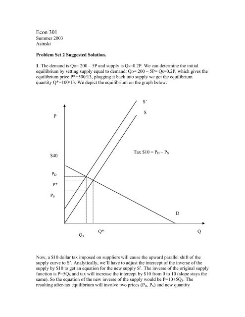
Econ 301Summer 2003AsinskiProblem Set 2 Suggested Solution.1. The demand is QD= 200 – 5P and supply is QS=0.2P. We can determine the initialequilibrium by setting supply equal to demand: QD= 200 – 5P= QS=0.2P, which gives theequilibrium price P*=500/13, plugging it back into supply we get the equilibriumquantity Q*=100/13. We depict the equilibrium on the graph below:S’PS$40Tax $10 = P D – P SP DP*P SDQ TQ*QNow, a $10 dollar tax imposed on suppliers will cause the upward parallel shift of thesupply curve to S’. Analytically, we’ll have to adjust the intercept of the inverse of thesupply by $10 to get an equation for the new supply S’. The inverse of the original supplyfunction is P=5Q S and tax will increase the intercept by $10 from 0 to 10 (slope stays thesame). So the equation of the new inverse of the supply would be P=10+5Q S . Theresulting after-tax equilibrium will involve two prices (P D , P S ) and new quantity

exchanged Q T . To determine the new quantity we set old inverse demand equal to newinverse supply: P=10+5Q S =40 - 0.2Q D . Solving for Q gives Q T =75/13. Plugging backinto the inverse demand above gives P D =505/13 (you can obtain the same number byusing new inverse supply). Then we plug Q T into the old inverse supply to get P S =375/13= P D – 10. These two prices and quantity exchanged completely characterize the newafter-tax equilibrium. Now we can also study the incidence of this tax on consumers.We know that the consumers’ share of a tax is∆PD/∆tax=(505/13 - 500/13)/10 = 5/130=1/26.We also know that the share of the tax that consumers bear can be determined by usingthe formula∆PD/∆tax=η/(η-ε)or equivalently= slope of supply/(slope of supply -- slope of demand),where η is the supply elasticity and ε is the demand elasticity. For linear demand andsupply it is easier to use the second expression. So we have∆PD/∆tax= 0.2/(0.2-(-5))=0.2/5.2=(1/5)*(5/26)=1/26. So, we’ve been able to obtain thesame result using the elasticities formula. Notice that consumers’ share of this tax isalmost negligible. The reason for that is the fact that demand is much more elasticrelative to supply (demand is flat and supply is steep). This flexibility (elasticity) ofbuyers prevents sellers from passing the large share of a tax onto buyers.2. The demand for coconut oil is given by Q=1,200 – 9.5P + 16.2P P +0.2Y.Initially P=45, P P =31, Q=1,275. I said that you can use Y=1,000, but here it is actuallynot necessary because we won’t need income in our calculations.The demand elasticity ε=(∆Q/∆P)*(P/Q)=(slope of demand with respect to P)*(P/Q)==(-9.5)*(45/1,275)= - 0.335 (inelastic – rather steep on the graph).Cross-price elasticity γ= (∆Q/∆P P )*(P P /Q)=(slope of demand with respect to price ofpalm oil)* (P P /Q)=16.2*(31/1,275)=0.394 (the cross-price elasticity is positive, whichmeans that the palm oil is the substitute for coconut oil).3. Problems 18 and 19. The supply function of the form Q=B*P η is a general form of theconstant-elasticity supply with elasticity equal to η (it is very easy to check usingderivatives). Similarly, the demand function of the form Q=A*P ε is the general form ofthe constant-elasticity demand with elasticity equal to ε.The incidence of the $1 unit tax can be determined using the formula:∆PD/∆tax=η/(η-ε)or equivalently= slope of supply/(slope of supply -- slope of demand),In Problem 18 both supply and demand are constant elasticity. Therefore, it is easier touse first expression above and see that it doesn’t matter where supply intersects demandbecause both η and ε stay the same along each curve (observe that slopes are definitelydifferent at different possible points of intersection). The other special case would be

where both curves are linear. Then we can use the second expression (in terms of slopes)and claim that if both curves are linear it also doesn’t matter where demand intersectssupply because slopes stay the same along each curve (here, though, elasticities aredifferent for each potential point of intersection).In problem 19 one of the curves is constant-elasticity and the other is linear. In this casethe incidence does depend on where demand and supply intersect. To see that we can useany of the two formulas. In the first one, elasticity of supply will be constant no matterwhere we are initially but elasticity of demand will be different at different points. Usingthe second expression we can see that slope of demand is the same no matter where thecurves intersect but slope of supply is different at different points.4. The Utility function is given by U(B,Z)=B*Z. The preferences summarized by thisutility function exhibit Diminishing Marginal Rate of Substitution (MRS) property. Tosee this let us first derive the equation for any Indifference Curve. Let’s fix the utilitylevel at U=10. The equation for indifference curve is derived from B*Z=10, which givesB=10/Z:B, burritos per week1051IC (U=10)1210Z, pizzas per weekNow, if we start at point (Z=1, B=10), if we want to consume one additional Pizza andstay on the indifference curve we have to cut our consumption of Burritos to 5 (so that westill have U=10=2*5). The MRS (= - slope) is approximately -∆B/∆Z= 5/1= 5. The