Exploiting Hardware Performance Counters with Flow and Context ...

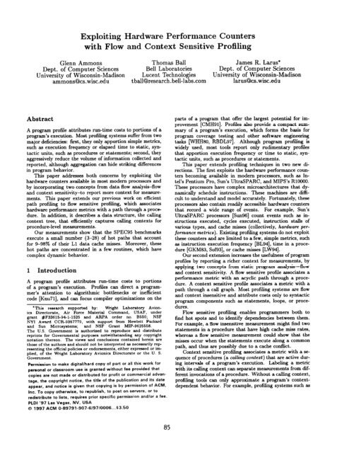
Exploiting Hardware Performance Counterswith Flow and Context Sensitive ProfilingGlenn Ammons Thomas Ball James R. Larus*Dept. of Computer Sciences Bell Laboratories Dept. of Computer SciencesUniversity of Wisconsin-Madison Lucent Technologies University of Wisconsin-Madisonammons@cs.wisc.edu tballQresearch.bell-labs.com larusQcs.wisc.eduAbstractA program profile attributes run-time costs to portions of aprogram’s execution. Most profiling systems suffer from twomajor deficiencies: first, they only apportion simple metrics,such as execution frequency or elapsed time to static, syntacticunits, such as procedures or statements; second, theyaggressively reduce the volume of information collected andreported, although aggregation can hide striking differencesin program behavior.This paper addresses both concerns by exploiting thehardware counters available in most modem processors andby incorporating two concepts from data flow analysis-flowand context sensitivity-to report more context for measurements.This paper extends our previous work on efficientpath profiling to flow sensitive pro!Xng, which associateshardware performance metrics with a path through a procedure.In addition, it describes a data structure, the callingcontext tree, that efficiently captures calling contexts forprocedure-level measurements.Our measurements show that the SPEC95 benchmarksexecute a small number (3-28) of hot paths that accountfor 9-98% of their Ll data cache misses. Moreover, thesehot paths are concentrated in a few routines, which havecomplex dynamic behavior.1 IntroductionA program profile attributes run-time costs to portionsof a program’s execution. Profiles can direct a programmer’sattention to algorithmic bottlenecks or inefficientcode [Knu71], and can focus compiler optimizations on the*This research supported by: Wright Laboratory AvionicsDirectorate, Air Force Material Command, USAF, undergrant #F33615-941-1525 and ARPA order no. B550; NSFNY1 Award CCR935’7779, with support from Hewlett Packardand Sun Microsystems; and NSF Grant MIP-9625558.The U.S. Government is authorized to reproduce and distributereprints for Governmental purposes notwithstanding any copyrightnotation thereon. The views and conclusions contained herein arethose of the authors and should not be interpreted as necessarily representing the official policies or endorsements, either expressed or implied,of the Wright Laboratory Avionics Directorate or the U. S.GovernmentPermission to make digital/hard copy of part or all this work forpersonal or classroom use is granted without fee provided thatcopies are not made or distributed for profit or commercial advan-tage, the copyright notice, the title of the publication and its dateappear, and notice is given that copying is by permission of ACM.Inc. To copy otherwise, to republish, to post on servers, or toredistribute to lists, requires prior specific permission and/or a fee.PLDl ‘97 Las Vegas, NV, USA0 1997 ACM 0-89791-907-6/9710006...$3.50parts of a program that offer the largest potential for improvement[CMHSl]. Profiles also provide a compact summaryof a program’s execution, which forms the basis forprogram coverage testing and other software engineeringtasks [WHHSO, RBDL97]. Although program profiling iswidely used, most tools report only rudimentary profilesthat apportion execution frequency or time to static, syntacticunits, such as procedures or statements.This paper extends profiling techniques in two new directions.The first exploits the hardware performance countersbecoming available in modem processors, such as Intel’sPentium Pro, Sun’s UltraSPARC, and MIPS’s RlOOOO.These processors have complex microarchitectures that dynamicallyschedule instructions. These machines are difficultto understand and model accurately. Fortunately, theseprocessors also contain readily accessible hardware countersthat record a wide range of events. For example, Sun’sUltraSPARC processors [Sun961 count events such as instructionsexecuted, cycles executed, instruction stalls ofvarious types, and cache misses (collectively, hardware performancemetrics). Existing profiling systems do not exploitthese counters and are limited to a few, simple metrics, suchas instruction execution frequency [BL94], time in a procedure[GKM83, Sof93], or cache misses [LW94].Our second extension increases the usefulness of programprofiles by reporting a richer context for measurements, byapplying two concepts from static program analysis-flowand context sensitivity. A flow sensitive profile associates aperformance metric with an acyclic path through a procedure.A context sensitive profile associates a metric with apath through a call graph. Most profiling systems are flowand context insensitive and attribute costs only to syntacticprogram components such as statements, loops, or procedures.Flow sensitive profiling enables programmers both tofind hot spots and to identify dependencies between them.For example, a flow insensitive measurement might find twostatements in a procedure that have high cache miss rates,whereas a flow sensitive measurement could show that themisses occur when the statements execute along a commonpath, and thus are possibly due to a cache conflict.Context sensitive profiling associates a metric with a sequenceof procedures (a calling contest) that are active duringintervals of a program’s execution. Labeling a metricwith its calling context can separate measurements from differentinvocations of a procedure. Without a calling context,profiling tools can only approximate a program’s contextdependentbehavior. For example, profiling systems such as85

gprof [GI

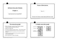
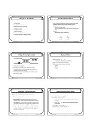
A2 0BO c2 0DEft1 0060FPathEncodingACDF 0ACDEFABCDF :ABCDEF 3ABDF 4 IABDEF 5 I(b)l=o-4sAIAIr+=2B CBCI=2r+=2l=‘4 43CL&DID1r+=lr+=lE FEFda3count[r]++count1 :m-+w69l=oFigure 1: Path profiling edge labelling and instrumentation. (a) An integer labelling with unique path sums; (b) The six paths andtheir path sums; (c) Simple instrumentation for tracking the path sums; (d) Optimized instrumentation for tracking the path sums.2.1 Path Profiling of Acyclic CFGsConceptually, the algorithm makes two linear-time traversalsof the CFG, visiting vertices in reverse topological orderin each pass. The two passes easily can be combined into asingle linear-time pass.In the first pass, each vertex w is labelled with an integerNP(v), which denotes the number of paths from w to EXIT.These values are well-defined because the graph is acyclic.As a base case, NP(EXZT) = 1. If v has successors wi...wUn(which are already labelled, since vertices are visited in reversetopological order), NP(w) = NP(wl) + ... + NP(wn).The second pass labels each edge e of the CFG with aninteger Vd(e) such that:• Every path from ENTRY to EXIT generates a pathsum in the range O...NP(ENTRY) - 1.• Every value in the range O...NP(ENTRY) - 1 is thepath sum of some path from ENTRY to EXIT.No processing is required for the EXIT vertex in this pass,as it has no outgoing edges. Consider vertex u with successorsWI ...wn. Since the algorithm traverses the CFG inreverse topological order, we may assume that for each Wi,all the edges reachable from wi have been labelled so thateach path from wi to EXIT generates a unique path sum inthe range O...NP(w;)- 1. Given a vertex tt, let u’s successorsbe totally ordered wi ...w., (the order chosen is immaterial).The value associated with edge ei = u + wi is simply thesum of the number of paths to EXIT from all successorsw1 .,.w;-1:Val(e;) = Cfz:NP(wj).Figure 2 illustrates the labelling process for a vertex uwith three successors, wi...ws. The paths from each wi toEXZT generate path sums in the range O...NP(wi)-1. Thelabel on edge u + wi is 0, so paths from v to EXIT beginningwith this edge will generate path sums in the rangeO...NP(wl) - 1. The label on edge u + wz is NP(wl), sopaths from u to EXIT beginning with this edge will generatepath sums in the range NP(w~)...NP(wI)+NP(w~)-1,and so on. Path sums for paths from u to EXIT thereforelie in the range O...NP(wl) + NP(w2) + NP(w3) - 1.I 0 ... NP(w) + NP(wJ + NP(w ) -I ii . ...-....- ..__ -A..---_-- __... L.-.-.;VFigure 2: Edge labelling phase.Given the edge labelling, the instrumentation phase isvery simple. An integer register r tracks the path sum andis initialized to 0 at the ENTRY vertex. Along an edgee with a non-zero value, r is incremented by Vd(e). Atthe EXIT vertex, r indexes an array to update a count(count[r]++) or serves as a hash key into a hash table ofcounters. For details on how to greatly reduce the numberof points at which r must be incremented, see [BL96, Bal94].2.2 Path Profiling of Cyclic CFGsCycles in a CFG introduce an unbounded number of paths.Every cycle contains a backedge, as identified by a depthfirstsearch from ENTRY. The algorithm only profilespaths that have no backedges or in which backedges occuras the first and/or last edge of the path. As a result, pathsfall into four categories:• A backedge-free path from ENTRY• A bra&edge-free path from ENTRYbackedge v -+ w;to EXIT;to V, followed by• After execution of backedge v + w, a backedge-freepath from w to z, followed by backedge z + y;• After executing backedge LJ + w, a backedge-free pathfrom w to EXIT.87

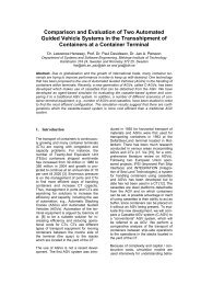
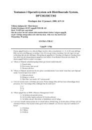
;;l hw-cnt = 0Figure 3: Instrumentation for measuring a metric over a paths.On out-of-order processors, such as the UltraSPARC, is is necessaryto read the hardware counter after writing it, to ensure thatthe write has completed.The algorithm of the previous section only guaranteesuniqueness of path sums for paths starting at a single “entry”point,. Paths with different starting points, such as thelatter three categories, may compute identical path sums.However, a simple graph transformation turns a cyclicCFG into an acyclic CFG and extends the uniqueness andcompactness properties of path sums to all paths describedabove, regardless of whether or not they are in the samecategory.For each backedge b = u + w in the CFG, the transformationremoves b from the CFG and adds two pseudo edgesin its place: b,,,,* = ENTRY -+ w and be,,d = v + EXIT.The resulting graph is acyclic and contains a bounded numberof paths. The pseudo edges represents paths that startand/or end with a backedge. For example, a path fromENTRY to vertex v, followed by backedge b = u + w inthe original CFG translates directly to a path starting atENTRY and ending with pseudo edge bend = v + EXIT.The path algorithm for acyclic CFGs runs on the transformed graph, labelling both original edges and pseudoedges. This labelling guarantees that all paths fromENTRY to EXIT have unique paths sums, including pathscontaining pseudo edges. After this labelling, instrumentationis inserted as before, with one exception. Since thepseudo edges do not represent actual transfers of control,they cannot. be instrumented. However, their values are incorporatedinto the instrumentation along a backedge:count [r+ENDI+;r=START,where END is the value of pseudo edge bend and STARTis the value of pseudo edge bat,,*.3 Flow Sensitive Profiling of HardwareMetricsThis section shows how to extend the path profiling algorithmto accumulate metrics other than execution frequency.These hardware metrics may record execution time, cachemisses, instruction stalls, etc. Although this discussion focuseson the UltraSPARC’s hardware counters [Sun96], similarconsiderations apply to other processors.3.1 Tracking Metrics Along a PathAssociating a hardware metric with a path is straightforward,as shown in Figure 3. At the beginning of a path, setthe hardware counter to zero. At the end of the path, readthe hardware counter and add its value into an accumulatorassociated with the path. Since paths are intraprocedural,hardware counters must be saved and restored at procedurecalls. A system can either save the counter before a call andrestore it after the call, or save the counter on procedureentry and restore it before procedure exit. Our implementationuses the latter approach to reduce code size and tocapture the cost of call instructions.The UltraSPARC provides an instruction that reads itstwo 32 bit hardware counters into one 64 bit general purposeregister. Several additional instructions are necessaryto extract the two values from the register. In total, ourinstrumentation requires thirteen or more instructions toincrement two accumulators and a frequency metric for apath.Both counters can be zeroed by writing a 64 bit registerto the two hardware counters. However, because ofthe UltraSPARC’s superscalar architecture, it, is necessaryto read the counters immediately after writing them, to ensurethat the write completes before subsequent instructionsexecute.’3.2 Measurement PerturbationAn important problem with hardware counters is the perturbationcaused by the instrumentation. As a simple example,consider using hardware counters to record instruction frequency.Each instrumentation instruction executed along apath is counted. Figure 3 shows an example, in which theprofiling instrumentation introduces two instructions alongpath A + B + D + F-one instruction for the read afterthe write to the hardware counters, and one instructionalong B + D.Moreover, instrumenting an executable introduces furtherperturbation. For example, path profiling requires afree local register in each procedure. If a procedure has nofree registers, EEL spills a register to the stack, which requiresadditional loads and stores around instructions thatoriginally used the register. These instructions affect a metric.In addition, EEL’s layout of the edited code can introducenew branches.For simple, predictable metrics, such as instruction frequency,a profiling tool can correct for perturbation by usingpath frequency to subtract the effect of instrumentationcode. For other metrics, however, it is very difficult to estimateperturbation effects. For example, if the metric isprocessor stalls or cache misses, separating instrumentationfrom the underlying behavior appears intractable. Moreover,instrumentation that executes at the beginning or endof a path, outside the measured interval, can also cause cacheconflicts that increase a program’s cache misses. We do nothave a general solution for this difficult problem, which hasbeen explored by others [MRW92]. Section 6 contains measurementsof the perturbation.3.3 OverflowThe UltraSPARC’s hardware counters are only 32 bits wide.A metric, such as cycle counts, can cause a counter to wrapin a few seconds. However, our intraprocedural instrumentationmeasures call-free paths, and even 32 bit counters‘Ashok Singhal, Sun Microsystems. Personal communication.Oct. 1996.88

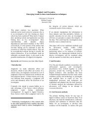
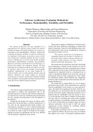
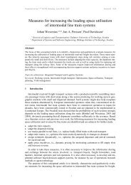
Figure 4: (a) A dynamic call tree, (b) its corresponding callgraph, and (c) its corresponding calling context tree.will not wrap on any conceivable path. Moreover, we accumulatedmetrics as 64 bit quantities, which will handle anyprogram.4 Context Sensitive ProfilingThis section describes the calling context tree (CCT), adata structure that compactly represents calling contexts,presents an algorithm for constructing a CCT, and showshow a CCT can capture flow sensitive profiling results andother performance metrics.4.1 The Calling Context TreeThe CCT offers an efficient intermediate point in the spectrumof run-time representations of calling behavior. Themost precise but space-inefficient data structure, as shownin Figure 4(a), is the dynamic call tree (DCT). Each treevertex represents a single procedure activation and can preciselyrecord metrics for that invocation. Tree edges representcalls between individual procedure activations. Thesize of a DCT is proportional to the number of calls in anexecution.At the other end of the spectrum, a dynamic call graph(DCG) (Figure 4(b)), compactly represents calling behavior,but at a great loss in precision. A graph vertex representsall activations of a procedure. A DCG has an edge X + Yiff there is an edge X + Y in the program’s dynamic calltree. Although the DCG’s size is bounded by the size ofthe program, each vertex accumulates metrics for (perhapsunboundedly) many activations. This accumulation leadsto the “gprof problem,” in which the metric recorded at aprocedure C cannot be accurately attributed to C’s callers.Furthermore, a call graph can contain “infeasible” paths,such as M + D + A + CY, which did not occur during theprogram’s execution.The calling contest tree (CCT) compactly represents allcalling contexts in the original tree, as shown in Figure 4(c).It is defined by the following equivalence relation on a pair ofvertices in a DCT. Vertices u and w in a DCT are equivalentif:• v and w represent the same procedure, and• the tree parent of v is equivalent to the tree parent ofw, or u = w.The equivalence classes of vertices in a DCT define the vertexset of a CCT. Let Eq(z) denote the equivalent class ofvertex 2. There is an edge Eq(u) + Eq(w) in the CCT iffthere is an edge u -+ w in the DCT.Figure 4(c) shows that the CCT preserves the two uniquecalling contexts associated with procedure C (M + A +B(b)CACB(a) (b) CC)Figure 5: (a) A dynamic call tree containing recursive calls, (b)its corresponding call graph, and (c) its corresponding callingcontext tree.C and M + D + C). A CCT contains a unique vertexfor each unique path (call chain) in its underlying DCT.Stated another way, a CCT is a projection of a dynamic calltree that discards redundant contextual information whilepreserving unique contexts. Metrics from identical contextswill be aggregated, again trading precision for space. A CCTcan accurately record a metric along different call pathstherebysolving the “gprof problem”. Another importantproperty of CCTs is that the sets of paths in the DCT andCCT are identical.As defined above, the out-degree of a vertex in the CCTis bounded by the number of unique procedures that maybe called by the associated procedure. Thus, the breadthof the CCT is bounded by the number of procedures in aprogram.’ In the absence of recursion, the depth of a CCTalso is bounded by the number of procedures in a program.However, with recursion, the depth of a CCT may be unbounded.To bound the depth of the CCT, we redefine vertexequivalence. Vertices u and w in a DCT are equivalentif:• u and w represent the same procedure, and• the tree parent of v is equivalent to the tree parentof w, or v = w, or there is a vertex u such that urepresents the same procedure as u and w and u is anancestor of both v and w.~The modified second condition ensures that all occurrencesof a procedure P below and including an instance of P inthe DCT are equivalent. As a result of this new equivalencerelation, the depth of a CCT never exceeds the number ofprocedures in a program since each procedure occurs at mostonce in any path from the root to a leaf of the CCT.The new equivalence relation introduces backedges intothe CCT, so it is not strictly a tree. However, CCTs neverinclude cross-edges or forward edges. This implies that treeedges are uniquely defined and separable from backedges.Unfortunately, backedges (which arise solely due to recursion)destroy the context-uniqueness property of a CCT withrespect to a DCT.Figure 5(a) shows a dynamic call tree with recursive callingbehavior and its corresponding call graph and CCT. Therecursive invocation of procedure A and its initial invocationare represented by the same vertex in the CCT.A space-precision trade-off in a CCT is whether to distinguishcalls to the same procedure from different call sites ina calling procedure. Distinguishing call sites requires more3The breadth of a DCT is unbounded due to loop iteration.‘A vertex is an ancestor of itself.89

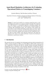
struct List;struct CallRecord;typedef union {List* le;CallRecord+ cr; int offset) Cellee;typedef union {CallRecord* cr; int offset) ListElem;struct CallRecord Cint ID; // procedure identifierCallRecord *parent; // tree parentint metrics[INJ ; // the metricsCallee children[l ; // the callees1;struct List CListElem pr;List *next;1;// list of dynamic calleesFigure 6: CCT data structures.space, but is useful for path profiling, as distinct intraproceduralpaths reach the different call sites. Other applicationsof a CCT may aggregate a metric for a pair of procedures,and would not benefit from this increased precision. Theapproach described below aSSumea that call sites are distinguished;changes to combine them are minor.4.2 Constructing a Calling Context TreeA CCT can be constructed during a program’s execution,as we now describe. Each vertex of a CCT is referred toas a “call record,” although different run-time activationrecords may share the same call record. Let CR be thecall record associated with the currently active procedureC. The principle behind building a CCT is simple: if D hasjust been called by C and is already represented by a recordthat is one of CR’s children, use the existing call record.Otherwise, look for a call record for D in C’s ancestors. Ifa record DR is found, the call to D is recursive, so createa pointer from CR to DR (a backedge), and make DR thecurrent call record. If 12 is not an ancestor of C, create anew call record DR for D and make it a child of CR.The first time that a new callee is encountered, we paythe cost of traversing the parent pointers. However, at subsequentcalls, a callee immediately finds its call record, regardlessof whether the call is recursive.The C structures in Figure 6 define the basic data typesin a CCT. A CallRecord contains two scalar fields and twoarrays:• ID is an int that identifies the procedure or functionassociated with the CallRecord. We currently usea procedure’s starting address its identifier, althoughmore compact encodings are possible.• parent is a pointer to the CallRecord’s tree parent.This pointer is NULL if the CallRecord represents theroot of the CCT.• metrics is an array of counters for recording metrics.The size of this array is usually fixed for allCallRecords. When combining path profiling with callgraph profiling, the size of the array depends on thenumber of paths in a procedure.(p=j?&6 D I, 1 IO lrn,*l --f---fizpzJFigure 7: A representation of the first two levels of the CCTfrom Figure 4. Dashed lines indicate pointers to lists and solidlines indicate pointers to call records. For simplicity, each cell isassumed to be four bytes wide.• children is an array of callee slots, one for each callsite in the procedure. Each slot may be a pointer toa list of children (for indirect calls), a pointer directlyto one child, or its uninitialized value-an offset to thestart of the call record. The low-order two bits of a slotform a tag that discriminates among the three possiblevalues.Figure 7 illustrates the CCT data structure for the firsttwo levels of the CCT in Figure 4, which includes the proceduresM, A and D. Each call record in the structure beginswith the corresponding procedure’s ID. The root of the CCTis labeled with the special identifier T, which corresponds tono procedure. The distinguished node is useful in two ways.First, our executable editing tool cannot insert the full instrumentationin start, which is a program’s entry point inUNIX. Second, if we extended our tool to handle signals, theCCT would need multiple roots, as signal handlers representadditional entry points into a program. The call record forthe root does not accumulate metrics.There are several ways to build a CCT. Our approach allowseach procedure to be instrumented separately, withoutknowledge of its callers or callees. Each procedure createsand initializes its own call records. When a procedure executesa call, the caller passes a pointer to the slot in its callrecord in which the callee should insert its call record. Ouralgorithm inserts instrumentation at the following points ina program in order to build a CCT:Start of program execution. The initialization code allocatesa heap for the CCT in a memory-mapped region. Theregion is demand paged, so physical memory is not allocateduntil it is actually used. The root call record is allocated andits callee slot is initialized to a list of one element, the offsetback to the beginning of the call record. Finally, a SPARCglobal register, called the callee slot pointer (gCSP), is setto the root’s call record. Callers use this register to pass apointer to a callee slot in the record down to the callee.Procedure entry. The instrumentation code first obtainsa pointer to the procedure’s call record. The code loads thevalue pointed to by the gCSP (the procedure’s callee slot).The low-order 2 bits of this value are a tag. If the tag is 0,the value is a pointer to a call record for this procedure.If the tag is 1, this procedure has not been called fromthis context. Masking off the low-order two bits yields anoffset from the beginning of the current call record (i.e.,the caller’s call record). The code then searches the parentpointers, looking for an ancestral instance of the callee.If a record is found, this call is recursive and the oldrecord is reused. If no record is found, the code allocatesand initializes a new call record. Initialization sets the IDand children fields of the new record. Callee slots for direct90

calls are set to the tagged offset of the slot in the record.Slots for indirect calls are set to a tagged pointer to a listcontaining a single entry, the tagged offset of the beginningof the call record. In both cases, the code stores a pointerto the found or allocated record in the callee slot.Finally, if the tag is 2, the callee slot contains a pointerto a list of callees. If this procedure has been called fromthis site before, its call record is in the list. The code movesits pointer to the front of the list, so it can be found morequickly next time. If there is no such pointer in the list,the list’s last element is the tagged offset to the caller’s callrecord. This provides enough information to follow the parentpointers and find or create a call record, as before.The callee’s call record becomes the new current callrecord, which is held in a local register call 1CRP. The instrumentationalso saves the gCSP to the stack. If an exceptionor signal transfers control to instrumented code, the normalexception mechanisms restore the 1CRP. If instead controltransfers to uninstrumented code, there is no 1CRP to restore.Thus, exceptions to instrumented code are handledtransparently, but the exception handling mechanism mustbe changed to handle exceptions to uninstrumented code.Signals, which have resumption semantics, do not have thisproblem.Procedure ezit. The instrumentation restores the oldgCSP from the stack. If an instrumented procedure A calls anuninstrumented procedure B, and B calls the instrumentedprocedures C and D, saving and restoring the gC8P ensuresthat C and D are correctly counted as children of A.Procedure call. The instrumentation sets the gCSP to thesum of the 1CRP and the offset to the callee slot for this callsite.Program ezit. Immediately before the program terminates,the instrumentation writes the heap containing theCCT to a 6le from which the CCT can be reconstructed.4.3 Associating Metrics with a CCTThe instrumentation code uses the metric fields in the currentcall record to capture metrics for the procedure invocation.The simplest metric is execution frequency, whichjust increments a counter in the CallRecord. To combineintraprocedural path profiles with calling context simply requiresa minor change to keep a procedure’s array of countersor hash table (Section 2) in a CallRecord.Recording hardware metrics is slightly trickier. Theleast expensive approach is to record a hardware counterupon entry to a procedure, and to compute and accumulatethe difference upon exit. This approach has two problems.First, it will not correctly measure functions thatare not returned to in the conventional manner (i.e., due tolongjmp’s or exceptions). Second, the measured interval extendsover the entire function invocation, which may cause32 bit counters to wrap. To avoid these problems, the instrumentationalso reads the hardware counters along loopbackedges. Although this has higher instrumentation costs,it produces more information and mitigates or eliminatesthese two problems.5 ImplementationWe implemented these algorithms in a tool called PP, whichinstruments SPARC binary executables to profile intraprocedural paths and call paths. PP is built using EEL (Exe-cutable Editing Library), which is a C++ library that hidesmuch of the complexity and system-specific detail of editingexecutables [LS95]. EEL provides abstractions that allowa tool to analyze and modify binary executables withoutbeing concerned with particular instruction sets, executabletile formats, or the consequences of deleting existing codeand adding foreign code (i.e., instrumentation).5.1 UltraSPARC Hardware CountersThe Sun UltraSPARC processors [Sun96] implement sixteenhardware counters, which record events such as instructionsexecuted, cycles executed, instruction stalls, andcache misses. The architecture also provides two programaccessibleregisters that can be mapped to two hardwarecounters, so a program can quickly read or set a counter,without operating system intervention. Solaris 2.5 currentlydoes not save and restore these counters or registers on acontext switch, so they measure all processes running on theprocessor. In our experiments, we minimized other activityby running a process locked onto a high-numbered processorof a SMP Server (low-number processors service interrupts).The 32 bit length of these counters is not a problem as PPrecords the hardware metrics along acyclic, intraproceduralpaths.6 Experimental ResultsThis section presents measurements of the SPEC95 benchmarks,made using PP. The benchmarks ran on a Sun UltraserverE5000-12 167MHz UltraSPARC processors and 2GBof memory-running Solaris 2.5.1. C benchmarks were compiledwith gee (version 2.7.1) and Fortran benchmarks werecompiled with Sun’s f77 (version 3.0.1). Both compilersused only the -0 option. In the runs, we used the ref inputdataset. Elapsed time measurements are for the entiredataset. Hardware metrics are for the entire run, or the lastinput file in the case of programs, such as gee, with multipleinput files.6.1 Run-Time OverheadThe overhead of intraprocedural path profiling is low (an averageof 32% overhead on the SPEC95 benchmarks, roughlytwice that of efficient edge profiling [BL94]). Details are reportedelsewhere [BL96]. The extensions described in thispaper increase the run-time cost of profiling, but the overheadsremain reasonable. Table 1 reports the cost of threeforms of profiling. Recording hardware metrics along intraproceduralpaths (Flow and HW) incurs an averageoverhead of 80%. Recording hardware metrics along withcall graph context (Context and HW) incurs an averageoverhead of 60%. Finally, recording path frequency (nohardware metrics) along with call graph context (Contextand Flow) incurs an average overhead of 70%.6.2 PerturbationPP’s instrumentation code can perturb hardware metrics.Table 2 reports a rough estimate of the perturbation forseveral metrics. The baseline in each case is the uninstrumentedprogram, which we measured by sampling theUltraSPARC’s hardware counters every six seconds (to avoid91

Benchmark099.go124.mSSksin-1126.gcc129.com press13O.li132.ijpeg134.perl147.vortexCINT96 AvglOl.tomcatY102.&mj103.su2cor104.hydro2d107.mgridllO.applu125.turb3d14l.apsi145.fPPPP146.~~~~5 635.6Base Flow and HW Context and HW Context and FlowTime Time Overhead Time Overhead Time Overhead(54 (s-3 (x base) (se4 (x base) (==I (x base)850.9 2517.0 3.0 1642.6 1.9 1949.2 2.3551.8 1446.9 2.6 1347.6 2.4 1011.4 1.8330.9 1461.5 4.4 1425.4 4.3 2984.5 9.0343.2 968.7 2.8 904.8 2.6 594.0 1.7479.5 1169.5 2.4 1270.4 2.6 961.2 2.0766.2 1494.0 1.9 1438.9 1.9 1130.7 1.5333.2 906.7 2.7 790.5 2.4 976.7 2.9648.1 1545.1 2.4 1672.4 2.6 1938.7 3.0538.0 1438.7 2.7 1311.6 2.4 1443.3 2.7-505.9 670.1 1.3 586.7 1.2 652.2 1.3693.0 786.7 1.1 766.9 1.1 793.5 1.1468.5 587.4 1.3 561.0 1.2 553.5 1.2795.6 1490.8 1.9 961.0 1.2 1147.1 1.4877.5 1088.6 1.2 1001.5 1.1 962.1 1.1710.1 1517.6 2.1 911.1 1.3 1293.3 1.8il1063.1 1847.6 1.7 1750.1 1.6 1452.2 1.4515.0 627.1 1.2 636.1 1.2 611.5 1.22090.4 2172.2 1.0 1978.4 0.9 2310.5 1.1815.8 1.3 741.6 1.2 773.9 1.21055.0 1.31284.1 1.8 1 1132.6 1.6 1227.6 1.795 vg 835.5SPEC95 Avg 703.3Table 1: Overhead of profiling. Base reports the execution time of the uninstrumented benchmark. Flow and HW reports the cost ofintraprocedural path profiling using hardware counters. Context and HW reports the cost of context sensitive profiling using hardwarecounters. Context and Flow reports the cost of context sensitive profiling using only frequency counts (no hardware counters).Cycles Insts DCache DCache ICacheF&ad Write MissBenchmark F C F C099.go 1.22 1.20 1.04 1.10124.m88ksim 1.38 1.33 1.21 1.17126.gcc 1.19 1.31 0.97 1.37129.compres.9 1.58 1.55 1.48 1.4013O.li 1.57 1.50 1.33 1.25132.ijpeg 1.18 0.83 1.04 0.80134.perl 1.77 1.49 1.52 1.18147.vortex 1.46 1.34 1.30 1.14mNTf.6 Avg 1.45 1.34 1.27 1.16lOl.tomcatv 1.12 1.05 1.13 1.04102.swim 1.06 1.07 1.05 1.05103.su2cor 1.06 1.06 1.07 1.04104.hydro2d 1.12 1.05 1.22 1.02107.mgrid 1.09 1.05 1.03 1.03llO.applu 1.25 1.03 1.21 1.06125.turb3d 1.39 1.14 1.13 1.0414l.apsi 1.02 0.98 1.08 1.02145.fPPPP 0.96 0.90 1.00 1.00146.wave5 1.07 0.98 1.11 1 .OlCFP95 Avg 1.10 1.01 1.09 1.03SPEC95 Avg 1.19 1.10 1.14 1.06Misses Misses StallsF C F C F C1.18 1.11 1.07 1.04 3.83 2.262.37 2.49 1.77 1.28 1.45 2.431.11 1.00 0.99 0.94 1.28 2.820.90 0.89 1.00 1.00 1.87 3.281.24 1.23 1.19 1.29 7.41 3.781.07 1.11 0.86 0.85 9.55 3.191.77 2.04 1.62 1.77 2.26 1.671.33 1.84 0.75 1.12 2.09 2.131.25 1.36 0.98 1.10 2.35 2.171.03 0.98 1.27 1.00 1.45 1.291.11 1.11 1.27 1.27 1.20 1.221.01 1.00 1.05 1.00 5.58 2.240.99 1.00 1.78 1.01 1.32 1.811.01 1.01 0.84 0.87 1.27 1.371.00 0.98 1.26 1.00 1.11 1.020.98 0.98 0.95 0.94 27.93 3.190.99 1.00 0.98 1.02 2.04 3.230.97 1.00 0.94 0.97 0.44 0.401.01 0.99 1.12 0.99 0.19 0.131.00 1.00 1.05 0.97 0.61 0.441.00 1.00 1.04 0.98 0.93 0.76‘hllspredict Store FPStalls Buffer StallsstallsF C F C F0.84 0.950.53 0.520.60 6.170.66 0.670.99 0.790.84 0.451.10 1.191.30 1.530.83 0.831.10 1.070.99 0.991.06 1 .oo0.20 2.301.01 2.341.11 1.020.99 0.961.02 1.870.97 0.970.67 0.530.96 1.120.86 0.900.04 0.490.00 18.540.05 130.690.31 0.3338.60 21.651.54 1.430.27 0.18C0.00 0.0010.741.13 1442.890.05 0.051.76 1.451.28 0.736.22 3.980.31 0.78 0.00 0.000.65 1.52 0.05 1.425.44 1.21 0.89 0.890.85 0.90 1.00 1.000.84 0.91 0.98 0.990.94 0.98 0.99 0.990.66 1.00 1.02 1.021.08 1.01 0.97 1.002.21 10.31 0.98 1.180.54 0.86 0.97 1.020.05 0.02 0.86 0.880.92 0.86 1.00 1.000.60 0.93 0.94 0.960.60 0.94 1 0.94 0.96Table 2: Perturbation of hardware metrics from profiling. F reports the ratio of each metric, recorded using flow sensitive profiling(intraprocedural paths), to the corresponding metric in the uninstrumented program. C reports the ratio of a metric, recorded usingcontext sensitive profiling (call graph paths), to the metric in the uninstrumented program.92

Benchmark099x0124&8gksim126.gcc129.compress13O.h132.ijpeg134.nerl147.bortexlOl.tomcatv102.swim103.su2cor104.hydro2d107.mgrid1 lO.appiu125.turb3d141 .apsi145.fPPPP146.wave5Size Nodesl.le7 268941.2e6 26172.le7 288638.9e4 2531 .oe6 32271.3e6 23113.6e6 55172.le8 2577102.5e5 7823.9e5 9508.8e5 18671.8e6 32556.5e5 12724.le5 11931.4e6 42958.5e6 124942.8e5 8061.5e6 2580Avg Avg Out Hew .ht I Ml&X I Call SiteNode Size Degree Avg MaX I Reolication I10.56.510.25.28.99.27.315.27.118.013.025.012.018.018.016.030.014.0930822817242835614753930511736.4 12.089 3071 15335.9 14.0118 5869 31277.1 16.0395 10488 44456.2 12.0269 3978 17026.2 12.0133 3768 22488.0 16.01305 9901 54098.2 18.02161 53148 205726.2 13.0107 2439 16437.8 15.0632 7942 3753!sOnePath322618682186720122521663463423186668476710592343773959227768136711676Table 3: Statistics for a CCT with intraprocedurai path information in the nodes. Size is size (in bytes) of the profile file. Nodes is thenumber of nodes in the CCT. Avg Node Size reports the average size of an allocated call record (bytes). Avg Out Degree reportsthe average number of children of interior nodes. Height reports the average and maximum height of the tree. Max Replicationreports the maximum number of distinct call records for any routine in the CCT. Finally, Call Sites reports the total number of callsites in all call records. Used is call sites that were actually reached. One Path is call sites that were reached in a given call record byexactly one path from the procedure’s entry.All Paths Hot PathsCold PathsDense Paths I Snarse PathsNum Inst Miss Num Inst Miss Num- Inst Miss Num Inst Miss26628 3.2elO l.le9 II 7 8.5% 13.1% 4 12.8% 8.2% 26617 78.7% 78.7%1115 7.8elO 6.3e8 22 28.9% 69.6% 2 20.2Yo 3.1% 1091 50.9% 27.3%126.gcc11769 1.7e8 3.8e6 3 4.3% 8.0% 0 0% 0% 11766 95.7% 92.0%129.compress249 Se10 1.3e9 11 34.0% 85.5% 4 19.6% 7.5% 234 46.4% 7.1%13O.h811 5.6elO l.le9 13 25.8% 58.7% 10 34.3% 21.7% 788 39.9% 19.6%132.ijpeg1284 3.6elO 1.6e8 11 37.3% 77.6% 1 3.2% 3.1% 1272 59.5% 19.2%134merl1427 2.5e10 6.7e8 20 27.3% 48.8% 8 14.4% 10.4% 1399 58.3% 40.8%147.;ortex ] 2244 7.3elO 1.2e9 14 39.3% 59.3% 3 15.5% 10.3% 2227 45.3% 30.4%CINT95 Avg 12.6 25.7% 52.6% 4.0 15.0% 8.0% 5674.2 59.3% 39.4%lOl.tomcatv 427 5.3elO 2.6e9 3 29.9% 62.7% 2 66.8% 34.9% 422 3.3% 2.4%102.swim 377 2.7elO 2.5e9 1 24.9% 50.9% 2 72.9% 47.0% 374 2.3% 2.1%103.su2cor 950 5.2elO 2.3e9 14 57.1% 83.3% 2 12.7% 9.8% 934 30.2% 6.8%104.hydro2d 1816 9.3elO 3.6e9 17 27.7% 53.9% 10 43.4% 28.4% 1789 28.9% 17.7%lO?.mgrid 588 1.4ell 3e9 9 7.4% 17.8% 2 87.5% 73.5% 577 5.1% 8.7%1 lO.applu 637 9.5elO 1.7e9 22 29.6% 74.1% 3 28.9% 8.2% 612 41.5% 17.7%125.turb3d 672 1.7ell 3.5e9 12 14.1% 72.9% 6 24.9% 11.2% 654 60.9% 15.9%14l.apsi 1065 5elO 1.8e9 15 24.5% 68.5% 3 7.7% 4.8% 1047 67.8% 26.7%145.fPPPP 1067 2.5ell 6.le9 5 51.3% 63.3% 7 24.1% 16.2% 1055 24.6% 20.5%146.wave5 934 6.3elO 3.le9 12 38.4% 62.9% 8 43.4% 24.5% 914 18.2% 12.6%CFP95 Avg 11.0 30.5% 61.0% 4.5 41.2% 25.9% 837.8 28.3% 13.1%SPEC95 Avg 11.7 28.4% 57.3% 4.3 29.6% 17.9% 2987.3 42.1% 24.8%SPEC95 Avg - go, gee 12.6 31.1 63.1 4.6 32.5 19.7 961.8 36.4 17.2Table 4: Ll data cache misses paths. Hot Paths are intraprocedural paths that incur at least 1% of a program’s cache misses. Coldpaths are the other paths. Dense Paths are hot paths that have an above average miss rate. Sparse paths are hot paths with abelow average miss rate. Num is the quantity of paths in the category. Inst is the instructions executed along these paths. Miss is theLl data cache misses along the path.93

Hot Procedures Cold ProceduresDense Procedures Sparse ProceduresBenchmark Num Path/Proc Misses Num Path/Proc Misses Num Path/Proc Misses099.go 9 182.9 30.7% 8 405.9 39.3% 394 55.2 29.9%124.mSSksim 12 18.0 77.2% 3 14.3 16.9% 207 4.1 5.9%126gcc 14 88.4 28.0% 10 155.1 16.1% 1055 8.5 55.9%129.compress 2 22.5 91.6% 4 6.5 7.9% 63 2.8 0.5%13O.li 9 6.0 66.1% 6 9.5 27.0% 242 2.9 6.9%132.ijpeg 9 42.2 86.9% 1 11.0 7.0% 255 3.5 6.1%134.perl 13 14.2 76.2% 6 16.7 14.1% 217 5.3 9.6%147.vortex 17 11.7 66.4% 4 2.2 12.2% 611 3.3 21.5%CINT95 Avg 10.6 48.2 65.4% 5.2 77.7 17.6% 380.5 10.7 17.0%lOl.tomcatv 1 41.0 99.7% 0 0.0 0.0% 142 2.7 0.3%102.swim 1 13.0 51.9% 2 12.0 48.0% 137 2.5 0.1%103.su2cor 8 32.4 90.1% 2 13.0 8.6% 196 3.4 1.4%104.hydro2d 7 20.0 46.8% 5 171.4 49.0% 213 3.8 4.1%107.mgrid 3 37.7 20.8% 2 7.0 78.9% 153 3.0 0.2%1 lO.applu 3 25.7 71.0% 3 33.0 28.9% 134 3.4 0.1%125.turb3d 11 7.5 80.7% 3 11.7 18.1% 171 3.2 1.2%14l.apsi 12 9.4 66.5% 5 12.8 26.1% 224 4.0 7.4%145.fPPPP 2 8.0 51.0% 3 222.3 47.9% 135 2.8 1.1%146.wave5 5 34.6 28.0% 3 32.3 68.5% 203 3.3 3.5%CFP95 Avg 5.3 22.9 60.6% 2.8 51.6 37.4% 170.8 3.2 1.9%SPEC95 Avg 7.7 34.2 62.8% 3.9 63.2 28.6% 264.0 6.5 8.6%-spEC95 Avg - go, gee 7.2 21.5 66.9% 3.2 36.0 28.7% 206.4 3.4 4.4%Table 5: Ll data cache misses per procedure. Hot Procedures incur at least 1% of a program’s cache misses. Dense Procedureshave above average miss ratios, while Sparse Procedures have below average miss ratios. Cold Procedures incur fewer than 1% ofa program’s cache misses. Path/Proc is the average number of paths executed in procedures in each category. Misses is the fractionof misses incurred by procedures in the category.counter wrap). These measurements also slightly perturbedthe hardware counters, as the data collection process suspendsthe application process and briefly runs. Since thehardware counters were set to only record user processesevents, the kernel was not directly measured. However, kernelcode could indirectly affect metrics, for example by pollutingthe cache.The table reports the ratio of each metric, collected withboth flow and context sensitive profiling, to the uninstrumentcdprogram. In some cases, instrumentation can improveperformance, for example by spreading apart storesand reducing store buffer stalls. The average perturbationfor ail metrics was small, though some programs exhibitedlarge errors. We have not yet isolated the cause of theseresults. However, it is encouraging that the two techniques,flow and context sensitive profiling, typically obtained similarresults.6.3 CCT StatisticsTable 3 contains information on the size of a CCT. Thisdata structure increases in size by a factor of 2-3x whenthe CCT is built on a call site basis. The total size of thedata structure is a few hundred thousand bytes for most ofthe benchmarks. However, the CCT can be quite large forprograms, such as 147.vortex, that contain many call paths.The table also shows that a CCT is a bushy, rather than tall,tree. In addition, the figures show that the routine with themost call records (Max Replication) often accounts for alarge fraction of the tree nodes.The final three columns report the total number of callsites in the allocated call records, how many of these sites areused, and how many sites only are reached by one intrapro-cedural path. The latter figure is particularly interesting,because in this case the combination of flow and contextsensitive profiling produces as precise a result as completeinterprocedural path profiling.6.4 Flow Sensitive ProfilingThis sections contains some sample measurements of hardwareperformance metrics along intraprocedural paths.Processor stalls have many manifestations-cache misses,branch mispredicts, load latency, or resource contentionbut,in general, they occur when operations with long latenciescannot be overlapped or when excessive contentionarises for resources. A processor’s dynamic scheduling logicdelays operations to preserve a program’s semantics or resolveresource contention. Compiler techniques, such astrace scheduling, instruction scheduling, or loop transformations,reorder instructions to reduce stalls. Most compilersoperate blindly, and apply these optimizations throughouta program, without an empirical basis for making tradeoffs.Our measurements show that this conventional approach isinefficient at best, as stalls are heavily concentrated on avery small number of paths, which we call hot paths.6.4.1 Cache Misses, By PathAs an example, Table 4 reports hot paths in the SPEC95benchmarks, for the UltraSPARC’s Ll data cache, which isan on-chip 16 Kb, direct mapped cache. Hot paths are intraproceduralpaths that incur at least 1% of the total cachemisses-this threshold is a parameter to control the numberof paths. Paths that are not hot are cold paths. A densepath is a hot path with a miss ratio above the program’s94

average miss ratio. A sparse path is a hot path with a belowaverage miss ratio. Sparse paths incur a large numberof misses because they execute heavily, rather than becauseof poor data locality. Dense paths are more common thansparse paths, which is fortunate because it seems likely thatdense paths are more likely to be optimized by a compiler.In the SPEC95 benchmarks, excepting 099.go and126.gcc, l-22 (avg. 12) dense paths account for 51-86%(avg. 63%) of the Ll cache misses. Considering all hot paths(dense + sparse) increases the number of paths to 3-28, butalso increase their coverage to 5998% (avg. 83%) of the Llmisses.The programs 099.go and 126.gcc have a well-known reputation for differing from the rest of the SPEC95 benchmarks.Our numbers corroborate this observation. Theyexecute roughly an order of magnitude more paths than theother programs and each path makes a less significant contributionto the program’s miss rate. It is therefore necessaryto reduce the threshold for hot paths to 0.1%. This changefinds 139 hot paths in 099.go that account for 55% of itsmisses and 172 hot paths in 126.gcc that account for 27%of its misses. In both cases, the number of hot paths is stillaround 1% of executed paths and a miniscule fraction ofpotential paths.6.4.2 Cache Misses, By ProcedureAnother way to apportion cache misses is by procedure. Table5 reports hot procedures in the SPEC95 benchmarks, forthe Ll data cache. A hot procedure incurs at least 1% of thecache misses. A dense procedure is a hot procedure that hasan above-average miss ratio. A sparse procedure is a hotprocedure with a below-average miss ratio.Again, cache misses are heavily concentrated in a smallportion of the program. From 1-24 (avg. 11.7) proceduresaccount for 4499% (avg. 91%) of the cache misses.This time, 099.go, 126.gcc, and 147.vortex have significantlylower coverage than the other programs. Again, lowering thethreshold to 0.1% improves coverage, so that 82 procedurescover 97% of the misses in 099.go, 157 procedures cover 89%of the misses in 126.gcc, and 75 procedures cover 96% of themisses in 147.vortex.6.4.3 Implications for ProfilingTable 5 also demonstrates that reporting cache misses byprocedure may not help isolate the aspects of a program’sbehavior that caused cache misses. Hot procedures executemany paths (an average of 34 and 63, for dense and sparseprocedures, respectively), so that knowing a procedure incursmany cache misses may not help isolate the path alongwhich they occur. Moreover, collecting and reporting cachemisses measurements at the statement level, in addition tobeing far more expensive than path profiling, does not alleviatethis problem. In these benchmarks, the basic blocksalong hot paths execute along an average of 16 differentpaths (of all type). Path profiling offers a low-cost way toprovide insight into a program’s dynamic behavior.7 Related WorkThis section describes previous work related to flow and contextsensitive profiling.7.1 Call-related Performance MeasurementMany profiling tools approximate context sensitive profilinginformation with heuristics. Tools such as gprof [GKM83]and qpt [BL94] use counts of the number of times that acaller invokes a callee to approximate the time in a procedureattributable to different callers. Because these profihng toolsdo not label procedure timings by context, information islost that cannot be accurately recovered. Furthermore, thetools also make naive assumptions when propagating timinginformation in the presence of recursion, which results infurther inaccuracy.Abnormalities that result from approximating contextsensitive information are well known [PF88]. Ponder andFateman propose several instrumentation schemes to solvethese problems. Their preferred solution associates proceduretiming with a (caIler, callee) pair rather than with asingle procedure. This results in one level of context sensitiveprofiling. Our work generalizes this to complete contexts.Pure Atria’s commercial profiling system Quantify uses arepresentation similar to a CCT to record instruction countsin procedures and time spent in system calIs @3en96]. Detailsand overheads of this system are unpublished. This workgoes further by incorporating path profiling and hardwareperformance metrics.7.2 Context Sensitive Measurement MechanismsCall path profiling is another approach to context sensitiveprofiling [Hal92, HG93]. It, however, differs substantiaIlyin its implementation and overhead. Hall’s schemere+instruments and re-executes programs to collect call pathprofiling of LISP programs in a top-down manner [Hal92].Initially, the call-sites in the “main” function are instrumentedto record the time spent in each callee. Once measurementshave been made, the system re-instruments theprogram at the next deepest level of the call graph and reexecutesit to examine particular behavior of interest, andso on. Since the amount of instrumentation is small, overheadintroduced in a run can be quite low. However, iterativere-instrumentation and r-e-execution can be impracticallyexpensive and does not work for programs with nonreproduciblebehavior. By contrast, our technique requiresonly one instrumentation and execution phase to recordcomplete information for all calling contexts.Goldberg and Hall used process sampling to record contextsensitive metrics for Unix processes [HG93]. By interruptinga process and tracing the call stack, they constructeda context for the performance metric. Beyond theinaccuracy introduced by sampling, their approach has twodisadvantages. Every sample requires walking the call stackto establish the context. Also, the size of their data StNCtureis unbounded, since each sample is recorded along withits call stack.7.3 Calling Context TreesCCTs are related to Sharir and Pnueli’s call strings, whichare sequences of calls used to label values for interproceduralflow analysis [SPSl]. In interprocedural analysis, the needto bound the size of the representation of recurs’ we programs95

and to define a distributive meet operator, made call stringsimpractical. CCTs, because they only need to capture asingle execution behavior, rather than all possible behaviors,are a practical data structure.Jerding, Stasko and Ball describe another approach forcompacting dynamic call trees that proceeds in a bottomupfashion [JSB97]. Using hash consing, they create a dagstructure in which identical subtrees from the call tree arerepresented exactly once in the dag. In this approach, twoactivations with identical contexts may be represented bydifferent nodes in the dag, since node equivalence is definedby the subtree rooted at a node rather than the path to anode.8 SummaryFlow and context sensitivity are used in data-flow analysis toincrease the precision of static program analysis. This paperapplied these techniques to a dynamic program analysisprogramprofiling-where they improve the precision of reportinghardware performance metrics. Previous tools associatedmetrics with programs’ syntactic components, whichmissed spatial or temporal interactions between statementsand procedures. Paths through a procedure or call graphcapture much of a program’s temporal behavior and providethe context to interpret hardware metrics.This paper showed how to extend our efficient pathprofiling algorithm to track hardware metrics along everypath through a procedure. In addition, it described a simpledata structure that can associate these metrics withpaths through a program’s call graph. Measurements of theSPEC95 benchmarks showed that the run-time overhead offlow and context sensitive profiling is reasonable and thatthese techniques effectively identify a small number of hotpaths that are the profitable candidates for optimization.The program paths identified by profiling have close tiesto compilation. Many compiler optimizations attempt to reducethe number of instructions executed on paths througha procedure [MR81, MW95, BGS97]. In order to ensureprofitability, these optimizations must not increase the totalinstructions executed along all paths through a procedureor, more strongly, over any path through a procedure. Inaddition, these optimizations duplicate paths to customizethem, which increases code size, to the detriment of high issuerate processors. Much of the optimization’s complexity,and many of their heuristics, stems from the assumptionthat all paths are equally likely. Compilers can use pathprofiles to identify portions of a program that would benefitfrom optimization, and as an empirical basis for makingoptimization tradeoffs.AcknowledgementsMany thanks to Ashok Singhal of Sun Microsystems for assistancein understanding and using the UltraSPARC hardwarecounters. Trishul Chilimbi, Mark Hill, and Chris Lbprovided helpful comments on this paper.References[Ba194] Thomas Ball. EfRciently counting program events withsupport for on-line queries. ACM !IYansactions onProgramming Languages and Systems, 16(5):1399-1410,September 1994.[Ben961[BGS97][BL94][BL961[CMHSl][GKM83][Ha1921[HG93][JSB97][Km711(Lsw[LW94][Mm11[MRW92][MW95]W-1[RBDL97][S&3][SP81][Sun961[WHHSO]Jim Bennett (PureAtria, Inc.). Personal communication,November 1996.Ft. Bodik, R. Gupta, and M. L. Soffa. Interprocedural conditionalbranch elimination. In Proceedings of the SIG-PLAN ‘97 Conference on Programming Language Designand Implementation, June 1997.T. Ball and J. Fl. Larus. Optimally profiling and tracingprograms. ACM pansactions on Programmrng Languagesand Systems, 16(3):1319-1360, July 1994.T. Ball and J. R. Larus. Efficient path profiling. In Proceedingsof MICRO 96, pages 46-57, December 1996.P. P. Chang, S. A. Mahlke, and W-M. W. Hwu. Usingprofile information to assist classic code optimizations.Software-Pmctice and Ezperience, 21(12):1301-1321, December 1991.S. L. Graham, P. B. Kessler, and M. K. McKusick. An executionprofiler for modular programs. Software-Practiceand Ezperience, 13:671-685, 1983.R. J. Hall. Call path profiling. In Proceedings of the14th International Conference on Software Engineering(ICSE92), pages 296-306,1992.R. J. Hall and A. J. Goldberg. Call path profiling of monctonicprogram resources in UNIX. In Proceedings of theUSENIX Summer 1993 Technrcal Conference, pages l-14., Cincinnati, OH, 1993.D. F. Jerding, J. T. Stasko, and T. Ball. Visualizing interactionsin program executions. In Proceedings of 1997International Conference on Softwan Engineering (toappear), May 1997.D. E. Knuth. An empirical study of FORTRAN pmgrams. Software-Practice and Ezperience, 1(2):105-133,June 1971.James R. Larus and Eric Schnarr. EEL: Machineindependentexecutable editing. In Proceedings of theSIGPLAN ‘95 Conference on Programming LanguageDesign and Implementation (PLDI), pages 291-300,June 1995.Alvin R. Lebeck and David A. Wood. Cache profiling andthe spec benchmarks: A case study. IEEE Computer,27(10):15-26, October 1994.E. Morel and C. Renvoise. Interprocedural elimination ofpartial redundancies. In S.S. Muchnick and N.D. Jones,editors, Program Flow Analysis: Theory and Applications.Prentice-Hall, Englewood Cliffs, NJ, 1981.Allen D. Malony, Daniel A. Reed, and Harry A. G. Wijshoff.Performance measurement instrusion and perturbationanalysis. IEEE ZYansactions on Parallel and DistributedSystems, 3(4):433-450, July 1992.F. Mueller and D. B. Whalley. Avoiding conditionalbranches by code replication. In Proceedings o,f the SIG-PLAN ‘95 Conference on Programming Language Designand Implementation, pages 56-66, June 1995.C. Ponder and R. J. ateman. Inaccuracies in programprofilers. Software-Practice and Ezpenence, 18:459467,May 1988.T. Reps, T. Ball, M. Das, and J. R. Larus. The use ofprogram profiling for software maintenance with applicktions to the year 2000 problem. In Technical Report 1335,Computer Sciences Department, University of Wisconsin,Madison, WI, January 1997.Pure Software. Quantify User’s Guide. 1993.Micha Sharir and Amir Pnueli. Two approaches to interproceduraldata flow analysis. In Steven S. Muchnick andNeil D. Jones, editors, Program Flow Analysis: Theoryand Apphcatrons, pages 189-233. Prentice-Hall, 1981.Sun Microelectronics. UltraSPARC User’s Manual, 1996.M. R. Woodward, D. Hedley, and M. A. Hennell. Experiencewith path analysis and testing of programs.IEEE lRonaactions on Software Engineering, 6(3):278-286, May 1980.96