Space Instrumentation: Microwave Spectroscopy - Max-Planck ...
Space Instrumentation: Microwave Spectroscopy - Max-Planck ...
Space Instrumentation: Microwave Spectroscopy - Max-Planck ...

You also want an ePaper? Increase the reach of your titles
YUMPU automatically turns print PDFs into web optimized ePapers that Google loves.
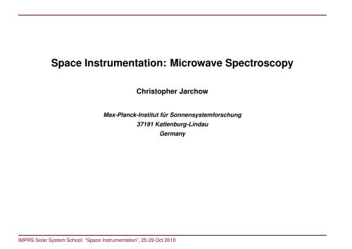
<strong>Space</strong> <strong>Instrumentation</strong>: <strong>Microwave</strong> <strong>Spectroscopy</strong><br />
Christopher Jarchow<br />
<strong>Max</strong>-<strong>Planck</strong>-Institut für Sonnensystemforschung<br />
37191 Katlenburg-Lindau<br />
Germany<br />
IMPRS Solar System School: “<strong>Space</strong> <strong>Instrumentation</strong>”, 25-29 Oct 2010
<strong>Microwave</strong> <strong>Spectroscopy</strong><br />
Oops, what’s this ?<br />
IMPRS Solar System School: “<strong>Space</strong> <strong>Instrumentation</strong>”, 25-29 Oct 2010 1
<strong>Microwave</strong> <strong>Spectroscopy</strong><br />
This is a ground-based microwave radiometer located at Northern Norway to detect the emission of<br />
atmospheric water vapour at 22 GHz (wavelength of 1.348 cm).<br />
I hope after these 45 minutes you have an idea how such an instrument works!<br />
By the way: From the data of this instrument we can derive the vertical distribution of H2O in the Earth’s atmosphere and its<br />
seasonal variation:<br />
IMPRS Solar System School: “<strong>Space</strong> <strong>Instrumentation</strong>”, 25-29 Oct 2010 2
Outline<br />
Outline<br />
• Motivation<br />
– Electromagnetic Spectrum<br />
• Fundamentals of <strong>Microwave</strong> Radiometers<br />
– Antenna<br />
– Heterodyne Receiver<br />
– Square-law Detector<br />
– Rayleigh-Jeans Approximation<br />
– Hot-Cold Calibration Technique<br />
– Receiver Noise Temperature<br />
• Spectrometer Technologies<br />
– Filter Bank<br />
– Acousto-Optical Spectrometer<br />
– Chirp Transform Spectrometer<br />
– Digital Autocorrelator<br />
– Fast Fourier Transform Spectrometer<br />
• Applications<br />
– Remote sensing of the Earth’s atmosphere<br />
– Radio Telescopes<br />
– SOFIA<br />
– HERSCHEL / HIFI<br />
IMPRS Solar System School: “<strong>Space</strong> <strong>Instrumentation</strong>”, 25-29 Oct 2010 3
Motivation<br />
Motivation<br />
IMPRS Solar System School: “<strong>Space</strong> <strong>Instrumentation</strong>”, 25-29 Oct 2010 4
Motivation<br />
We want to measure electromagnetic radiation intensity Iν received from a certain solid angle ∆Ω around a certain direction by<br />
an absorbing area ∆A within a certain frequency range ∆ν:<br />
Iν def<br />
=<br />
Pν<br />
∆A · ∆ν · ∆Ω<br />
�<br />
W<br />
m 2 �<br />
· Hz · sr<br />
IMPRS Solar System School: “<strong>Space</strong> <strong>Instrumentation</strong>”, 25-29 Oct 2010 5
Motivation<br />
We are interested in the microwave region (30–3000 GHz frequency, 10–0.1 mm wavelength), because molecules interact with<br />
this radiation by changing their rotational quantum state. Each molecule has a characteristic pattern of transition frequencies<br />
(spectral lines) and can be uniquely identified.<br />
Vibration-rotation energy diagram. Vibration-rotation spectrum of CO.<br />
IMPRS Solar System School: “<strong>Space</strong> <strong>Instrumentation</strong>”, 25-29 Oct 2010 6
Fundamentals of <strong>Microwave</strong> Radiometers<br />
Fundamentals of <strong>Microwave</strong> Radiometers<br />
IMPRS Solar System School: “<strong>Space</strong> <strong>Instrumentation</strong>”, 25-29 Oct 2010 7
Antenna<br />
<strong>Microwave</strong> receivers work quite similar like an ordinary radio: First we need an antenna to couple the electromagnetic wave from<br />
free space into a wire structure, often a coaxial cable. This is most often done using a so-called horn antenna.<br />
Depending on the wavelength horn antennas can be quite small . . .<br />
Note the small SMA connector for the coax-cable.<br />
IMPRS Solar System School: “<strong>Space</strong> <strong>Instrumentation</strong>”, 25-29 Oct 2010 8
Antenna<br />
. . . or pretty big:<br />
The Horn Antenna at Bell Telephone Laboratories in Holmdel, New Jersey, with which Arno<br />
Penzias and Robert Wilson discovered the cosmic microwave background radiation in 1964.<br />
IMPRS Solar System School: “<strong>Space</strong> <strong>Instrumentation</strong>”, 25-29 Oct 2010 9
Heterodyne Receiver<br />
T a<br />
Block diagram of a total power radiometer<br />
Antenna Mixer<br />
RF IF<br />
LO<br />
Local Oscillator<br />
IF Amplifier Filter Square-Law Detector DC Amplifier<br />
P ~ T n +T a<br />
The antenna produces a voltage proportional to the incident electric field pattern of the radio frequency (RF):<br />
URF (t) = E · cos(2πνt + Φ)<br />
The task of the mixer is to multiply the RF signal with a local oscillator signal ULO(t):<br />
ULO(t) = Q · cos(2πνLOt + ΦLO)<br />
The mixer can be any device with a non-linear I(U) characteristic, for example a simple diode:<br />
Now insert<br />
I(U) = Is · (e −U/U0 − 1)<br />
= Is ·<br />
⎛<br />
⎝ 1<br />
U<br />
1!<br />
U0<br />
+ 1<br />
� �2<br />
U<br />
+<br />
2! U0<br />
1<br />
� �3<br />
U<br />
+ . . . +<br />
3! U0<br />
1<br />
� �n<br />
U<br />
n! U0<br />
= a1U + a2U 2 + a3U 3 + . . . + anU n + . . .<br />
U(t) = URF (t) + ULO(t)<br />
IMPRS Solar System School: “<strong>Space</strong> <strong>Instrumentation</strong>”, 25-29 Oct 2010 10<br />
+ . . .<br />
⎞<br />
⎠
Heterodyne Receiver<br />
I(U) = a1(URF (t) + ULO(t)) + a2(URF (t) + ULO(t)) 2 + a3(URF (t) + ULO(t)) 3 + . . . + an(URF (t) + ULO(t)) n + . . .<br />
Important is the second order (quadratic) term:<br />
I(t) = . . .<br />
+a2 (E · cos(2πνt + Φ) + Q · cos(2πνLOt + ΦLO)) 2<br />
+ . . .<br />
= . . .<br />
a2E 2 · cos 2 (2πνt + Φ)<br />
+2a2EQ cos(2πνt + Φ) · cos(2πνLOt + ΦLO)<br />
+a2Q 2 cos 2 (2πνLOt + ΦLO)<br />
+ . . .<br />
= . . .<br />
+a2EQ [cos(2π(ν − νLO)t + Φ − ΦLO) + cos(2π(ν + νLO)t − Φ + ΦLO)]<br />
+ . . .<br />
➠ The mixer creates the sum and difference frequencies of the RF and LO frequency!<br />
IMPRS Solar System School: “<strong>Space</strong> <strong>Instrumentation</strong>”, 25-29 Oct 2010 11
Heterodyne Receiver<br />
By inserting a bandpass filter with bandwidth ∆ν = ν2 −ν1 at the output of the mixer we can select only the term with the difference<br />
frequency, the so-called intermediate frequency:<br />
ν1 ≤ |ν − νLO| ≤ ν2<br />
Hence, after mixing and filtering the output signal of the receiver is:<br />
or:<br />
I(t) ∝ EQ cos(2π(ν − νLO)t + Φ − ΦLO)<br />
I(t) ∝ EQ cos(2π(νLO − ν)t − Φ + ΦLO)<br />
Important: The difference frequency is low enough (about 1 to 4 GHz) to be amplified and processed by existing electronics!<br />
IMPRS Solar System School: “<strong>Space</strong> <strong>Instrumentation</strong>”, 25-29 Oct 2010 12
Heterodyne Receiver<br />
Bad effect of the mixing process:<br />
The intermediate signal contains always signal from two different frequency ranges, the so-called upper sideband and lower<br />
sideband! Thus a heterodyne receiver is usually always a double sideband receiver and assigning the original frequency to a<br />
spectral feature is not unique.<br />
Final step: Square-law detector<br />
To measure the power of the IF-signal we just need to square it (P = U 2 /R or P = RI 2 ) and average the fluctuating signal over<br />
some short time ∆t (running mean). As seen before this could be done using a diode (hence the symbol of a diode).<br />
The resulting final voltage is proportional to the power of the incident RF-signal at the antenna and can be digitized using standard<br />
analog-to-digital converters.<br />
IMPRS Solar System School: “<strong>Space</strong> <strong>Instrumentation</strong>”, 25-29 Oct 2010 13
Calibration<br />
So far we have an output signal proportional to the power of the incident RF-signal. But this signal depends on the gain of the<br />
amplifiers used, and varies with gain drifts (ie.g. caused by changing room temperature).<br />
➠ We need to calibrate the recorded output signal somehow into physical units!<br />
Idea: Let’s look at the thermal emission of a blackbody with the heterodyne receiver!<br />
The idea is based on the fact that the power radiated by a blackbody within a narrow frequency interval is proportional to its<br />
temperature as long as hν ≪ kT (Rayleigh-Jeans approximation) is valid:<br />
P (T, ν) = 2hν3<br />
c 2 ·<br />
= 2hν3<br />
c 2 ·<br />
� 2kν2<br />
c 2 · T<br />
1<br />
e hν/kT − 1<br />
1<br />
(1 + hν/kt + . . .) − 1<br />
IMPRS Solar System School: “<strong>Space</strong> <strong>Instrumentation</strong>”, 25-29 Oct 2010 14
Calibration<br />
This means the radiation power indicated by our heterodyne receiver can be written as a linear function of the temperature of the<br />
blackbody we are looking at:<br />
P = const · (T + Tn)<br />
Using two blackbodies at different temperatures – the so-called hot load and cold load we can assign any indicated power an<br />
equivalent blackbody temperature:<br />
P h<br />
P a<br />
P c<br />
-T n T c T a T h<br />
Ta = Th(Pa−Pc) − Tc(Pa−Ph)<br />
Ph−Pc<br />
In addition we obtain the receiver noise temperature Tn (the power which the receiver indicates without any input signal) – this<br />
is thermal mixer and amplifier noise:<br />
Tn = Th Pc−Tc Ph<br />
Ph−Pc<br />
IMPRS Solar System School: “<strong>Space</strong> <strong>Instrumentation</strong>”, 25-29 Oct 2010 15
Calibration<br />
This calibration is the reason why in microwave radiometry/spectroscopy the radiation intensity is always stated in terms of<br />
temperature!<br />
The theoretically lowest (i.e. best) receiver noise temperature is given by the quantum limit Tn = hν/k.<br />
Example:<br />
Double sideband (DSB) receiver noise temperatures for the HIFI instrument onboard the HERSCHEL space observatory. SIS<br />
stands for a superconductor-insulator-superconductor mixer, HEB stands for hot-electron-bolometer mixer. These two mixer<br />
technologies provide much lower receiver noise temperatures than a Schottky diode mixer.<br />
Note: Noise temperatures are several ten to several thousands of Kelvin, but the signal to be detected is usually only several ten<br />
milli-Kelvin up to a few Kelvin large! The mixer noise creates most of the observed output power of the receiver!<br />
IMPRS Solar System School: “<strong>Space</strong> <strong>Instrumentation</strong>”, 25-29 Oct 2010 16
Spectrometer Technologies<br />
Spectrometer Technologies<br />
IMPRS Solar System School: “<strong>Space</strong> <strong>Instrumentation</strong>”, 25-29 Oct 2010 17
Spectrometer: Filterbank<br />
Sow far we have a receiver with a single output number – a single channel radiometer.<br />
To get a spectrum composed of many channels the simplest technical approach is a filterbank:<br />
Each filter has a different passband characteristic which determines center frequency and resolution of the corresponding spectral<br />
channel.<br />
If we reduce the bandwidth of the passband filter we can increase the spectral resolving power R = ∆ν/ν of a heterodyne<br />
receiver to nearly arbitrarily high numbers (up to 10 7 is already standard). This is different from e.g. an optical grating!<br />
Useful resolutions for observations of planetary atmospheres and comets are 1 MHz – 50 kHz!<br />
IMPRS Solar System School: “<strong>Space</strong> <strong>Instrumentation</strong>”, 25-29 Oct 2010 18
Spectrometer: Acousto-Optical Spectrometer (AOS)<br />
An Acousto Optical Spectrometer (AOS) is based on the diffraction of light at ultrasonic waves. A<br />
piezoelectric transducer, driven by the IF signal (from the receiver), generates an acoustic wave in<br />
a crystal (the so-called Bragg-cell). This acoustic wave modulates the refractive index and induces<br />
a phase grating. The Bragg-cell is illuminated by a collimated laser beam. The angular dispersion<br />
of the diffracted light represents a true image of the IF-spectrum according to the amplitude and<br />
wavelengths of the acoustic waves in the crystal. The spectrum is detected by using a single<br />
linear diode array (CCD), which is placed in the focal plane of an imaging optics.<br />
taken from http://en.wikipedia.org/wiki/Acousto Optical Spectrometer<br />
IMPRS Solar System School: “<strong>Space</strong> <strong>Instrumentation</strong>”, 25-29 Oct 2010 19
Spectrometer: Chirp Transform Spectrometer (CTS)<br />
Chirp Transform Spectrometers are based on Surface Acoustic Wave (SAW) filters.<br />
These filters can be created in such a way, that a delta pulse as input signal shows up as a chirp output signal (linear increasing<br />
frequency versus time). If such a signal is put into another so-called matched SAW-filter, which would create a similar, but<br />
decreasing chirp signal, then the output would be a delta pulse again.<br />
Mixing the increasing chirp signal with a continous wave (CW) signal will shift the chirp signal in frequency and as finally the<br />
moment in time when the delta pulse apears as output of the matched filter. This behaviour is used to analyze the frequency of<br />
the CW-signal, and finally to use this filter combination as spectrometer.<br />
IMPRS Solar System School: “<strong>Space</strong> <strong>Instrumentation</strong>”, 25-29 Oct 2010 20
Spectrometer: Digital Autocorrelator Spectrometer (ACS)<br />
A digital autocorrelator is the digital version of an analog Fourier Transform Spectrometer. Using a fast analog-to-digital converter<br />
(only 1 or 2 bit resolution) a short time interval ∆t of the IF-signal is sampled with N data points. A highly specilized digital circuit<br />
calculates the autocorrelation function (as with an analog Fourier Transform Spectrometer this step creates an interferogram.<br />
These two steps are repeated and all the interferograms are co-added.<br />
Finally the Fourier Transform of the interferogram provides the power spectrum of the IF-signal (Wiener-Khinchin-Theorem).<br />
Visualisation of the “Wiener-Khinchin-Theorem”.<br />
IMPRS Solar System School: “<strong>Space</strong> <strong>Instrumentation</strong>”, 25-29 Oct 2010 21
Spectrometer: Fast Fourier Transfrom Spectrometer (FFTS)<br />
In the last few years the <strong>Max</strong>-<strong>Planck</strong>-Institut für Radioastronomie in Bonn developed spectrometers,<br />
which perform a real-time digital fast fourier transformation of the IF-signal. This technology<br />
became possible with the development of extremely fast analog-to-digital converters and field<br />
programmable gate arrays (FPGAs).<br />
In general a short time intervall of the IF-signal is digitized and then a highly specilized digital<br />
circuit calculates the spectrum using the Fast Fourier Transform algorithm. The trick is to do this<br />
transformation as fast as the sampling of the IF, that means transforming a sample of length ∆t<br />
does not take longer than a duration ∆t. No time gaps, no loss of IF-signal!<br />
However, this technology needs further developments to survive space environment!<br />
IMPRS Solar System School: “<strong>Space</strong> <strong>Instrumentation</strong>”, 25-29 Oct 2010 22
Application of <strong>Microwave</strong> Heterodyne Receivers<br />
Applications<br />
IMPRS Solar System School: “<strong>Space</strong> <strong>Instrumentation</strong>”, 25-29 Oct 2010 23
Ground-based Remote Sensing of the Earth’s Atmosphere<br />
We observe the thermal emission of atmospheric H2O when the molecule transits between two rotational quantum states.<br />
Profile information in the spectra: The line width is proportional to the<br />
atmospheric pressure (altitude information), the line amplitude is proportional<br />
to the molecule’s abundance (mixing ratio information).<br />
Mesosphere<br />
Stratosphere<br />
Troposphere<br />
decreasing<br />
line width<br />
increasing<br />
line width<br />
observed total<br />
line intensity<br />
IMPRS Solar System School: “<strong>Space</strong> <strong>Instrumentation</strong>”, 25-29 Oct 2010 24
<strong>Space</strong>-based Remote Sensing of the Earth’s Atmosphere<br />
Remote sensing of the Earth’s atmosphere has been also done extensively from space!<br />
Advantages:<br />
1. Global coverage<br />
2. Scanning the limb of the atmosphere with a narrow antenna beam gives additional altitude information and better altitude<br />
resolution of the ob<br />
Here needs to be named the <strong>Microwave</strong> Limb Sounder (MLS) onboard the Upper Atmosphere Research Satellite (UARS,<br />
launched 1991) and the second generation MLS instrument onboard the AURA satellite (launched 2004).<br />
IMPRS Solar System School: “<strong>Space</strong> <strong>Instrumentation</strong>”, 25-29 Oct 2010 25
Radio Telescopes<br />
Heinrich Hertz Telescope, Arizona<br />
Effelsberg 100m close to Bonn<br />
James Clerk <strong>Max</strong>well Telescope, Hawaii<br />
IRAM 30m close to Granada, Spain<br />
IMPRS Solar System School: “<strong>Space</strong> <strong>Instrumentation</strong>”, 25-29 Oct 2010 26
Radio Telescopes<br />
Remember: a radio telescope dos not provide images, but instead the spectrum of a single pixel!<br />
Images can be only obtained by slowly rastering across the sky.<br />
Detection of H2CO and HCN in the coma of Hale-Bopp, observed 1997 at the Heinrich Hertz Telescope with<br />
a CTS as spectrometer.<br />
IMPRS Solar System School: “<strong>Space</strong> <strong>Instrumentation</strong>”, 25-29 Oct 2010 27
Radio Telescopes<br />
Water vapour and oxygen in the Earth’s atmosphere prohibit clear view of the sky!<br />
IMPRS Solar System School: “<strong>Space</strong> <strong>Instrumentation</strong>”, 25-29 Oct 2010 28
SOFIA: an airborne far-infrared (FIR) telescope<br />
SOFIA<br />
IMPRS Solar System School: “<strong>Space</strong> <strong>Instrumentation</strong>”, 25-29 Oct 2010 29
MIRO: a tiny radio telescope onboard ROSETTA<br />
Even the ROSETTA spacecraft towards comet 67P/Churyumov-Gerasimenko carries a tiny radio telescope!<br />
IMPRS Solar System School: “<strong>Space</strong> <strong>Instrumentation</strong>”, 25-29 Oct 2010 30
MIRO: a tiny radio telescope onboard ROSETTA<br />
IMPRS Solar System School: “<strong>Space</strong> <strong>Instrumentation</strong>”, 25-29 Oct 2010 31
MIRO: a tiny radio telescope onboard ROSETTA<br />
IMPRS Solar System School: “<strong>Space</strong> <strong>Instrumentation</strong>”, 25-29 Oct 2010 32
MIRO: CTS developed 1997–2000 at MPS<br />
MIRO analog tray<br />
IMPRS Solar System School: “<strong>Space</strong> <strong>Instrumentation</strong>”, 25-29 Oct 2010 33
HERSCHEL / HIFI<br />
HERSCHEL Specifications<br />
Height 9 m (29.53 ft)<br />
Width 4.5 m (14.76 ft)<br />
Launch Mass 3300 kg (7275.25 lbs)<br />
Power 1 kW<br />
Launch Vehicle Ariane 5<br />
Orbit Lissajous around L2<br />
Science Data Rate 100 kbs<br />
Telescope Diameter 3.5 m (11.48 ft)<br />
Telescope WFE 0 µm (goal 6 µm)<br />
Telescope Temperature 0 to 90 K (-334 ◦ to -298 ◦ F)<br />
ABS Pointing (68%) 3.7” (goal < 1.5”)<br />
REL Pointing (68%) 0.3”<br />
Helium II Temperature 1.65 K (-456.7 ◦ F)<br />
Lifetime in L2 (spec) 3 yrs<br />
IMPRS Solar System School: “<strong>Space</strong> <strong>Instrumentation</strong>”, 25-29 Oct 2010 34
HERSCHEL / HIFI<br />
Herschel is orbiting the sun at the second Lagrangian point L2.<br />
IMPRS Solar System School: “<strong>Space</strong> <strong>Instrumentation</strong>”, 25-29 Oct 2010 35
HERSCHEL / HIFI<br />
Details of the HERSCHEL cryostat. It contains the three instruments HIFI, PACS, SPIRE,<br />
and about 2300 litres of superfluid Helium for detector cooling.<br />
IMPRS Solar System School: “<strong>Space</strong> <strong>Instrumentation</strong>”, 25-29 Oct 2010 36
HERSCHEL / HIFI<br />
Integration of the three instruments HIFI, PACS, SPIRE into the cryostat. The HIFI Focal<br />
Plane Unit (FPU) can be seen close to the center of the image.<br />
IMPRS Solar System School: “<strong>Space</strong> <strong>Instrumentation</strong>”, 25-29 Oct 2010 37
HERSCHEL / HIFI<br />
HIFI blockdiagram showing the various sub systems and their interconnections.<br />
HIFI observes two polarizations with two different spectrometers: The High Resolution Spectrometer<br />
(HRS) is a digital autocorrelator, the Wideband Spectrometer (WBS) is an acoustooptical<br />
spectrometer. Only the FPU needs to be cooled and is placed inside the cryostat.<br />
IMPRS Solar System School: “<strong>Space</strong> <strong>Instrumentation</strong>”, 25-29 Oct 2010 38
HERSCHEL / HIFI<br />
Optical design of the Wideband Spectrometer (WBS).<br />
IMPRS Solar System School: “<strong>Space</strong> <strong>Instrumentation</strong>”, 25-29 Oct 2010 39
HERSCHEL / HIFI<br />
Technical realization of the optical bench of the Wideband Spectrometer WBS. The laser<br />
is at the right and the four-line CCD at the left.<br />
IMPRS Solar System School: “<strong>Space</strong> <strong>Instrumentation</strong>”, 25-29 Oct 2010 40
HERSCHEL / HIFI<br />
The HIFI / WBS Electronics Box was built at MPS.<br />
IMPRS Solar System School: “<strong>Space</strong> <strong>Instrumentation</strong>”, 25-29 Oct 2010 41
HERSCHEL / HIFI<br />
Functional testing of the WBS electronic box at the MPS in the microwave laboartory (R-Building).<br />
IMPRS Solar System School: “<strong>Space</strong> <strong>Instrumentation</strong>”, 25-29 Oct 2010 42
HERSCHEL / HIFI<br />
signal/continuum<br />
signal/continuum<br />
1.05<br />
1.00<br />
0.95<br />
0.90<br />
0.85<br />
0.02<br />
0.01<br />
0.00<br />
-0.01<br />
O2 5,4-3,4<br />
-0.02<br />
773.70 773.75 773.80 773.85 773.90 773.95 774.00<br />
frequency (GHz)<br />
First results: Molecular oxygen (O2) on Mars observed with HIFI / WBS; 1400 ± 120 ppm confirmed.<br />
IMPRS Solar System School: “<strong>Space</strong> <strong>Instrumentation</strong>”, 25-29 Oct 2010 43
<strong>Space</strong> <strong>Instrumentation</strong>: <strong>Microwave</strong> <strong>Spectroscopy</strong><br />
Thank You!<br />
IMPRS Solar System School: “<strong>Space</strong> <strong>Instrumentation</strong>”, 25-29 Oct 2010 44