
You also want an ePaper? Increase the reach of your titles
YUMPU automatically turns print PDFs into web optimized ePapers that Google loves.
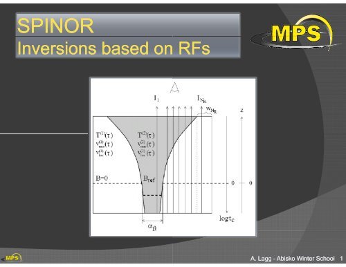
<strong>SPINOR</strong><br />
Inversions based on RFs<br />
A. Lagg - Abisko Winter School 1
Asymmetric profiles and ME (1) )<br />
MHD MHD-Simulations Simulations (Vögler et al. 2005)<br />
)<br />
A. Lagg - Abisko Winter School 2
Asymmetric profiles and ME (2) )<br />
MHD MHD-Simulations Simulations (Vögler et al. 2005)<br />
)<br />
� Fe I 630.1 and 630.2 profiles<br />
degraded to SP pixel size<br />
� Maps of inferred B and v<br />
very similar to real ones!<br />
� Maps of inferred B and v LOS<br />
A. Lagg - Abisko Winter School 3
Inversions with gradients<br />
� Inversion codes capable of f deealing<br />
with gradients<br />
� Are based on numerical solution<br />
of RTE<br />
�� Provide reliable thermal info ormation<br />
� Use less free parameters thhan<br />
ME codes (7 vs 8)<br />
�� Infer stratifications of physic cal parameters with depth<br />
� Produce better fits to asymmmetric<br />
Stokes profiles<br />
� Height dependence of atmosppheric<br />
parameters is needed for<br />
� easier solution of the 180 o a<br />
� 3D structure of sunspots annd<br />
pores<br />
� Magnetic flux cancellation eevents<br />
� Polarity inversion lines<br />
� Dynamical state of coronal<br />
� wave propagation analysis<br />
� …<br />
azimuth disambiguity g y<br />
loop footpoints<br />
A. Lagg - Abisko Winter School 4
Example: SIR inversion<br />
+<br />
• Spatial resolution: ∼0.4"<br />
VIP TESOS KAOS<br />
1.0<br />
0.8<br />
0.6<br />
0.4<br />
Stok tokes I/I I/IQS Stokes V/I V/IQS 0.2<br />
0 20 40 4 60 80<br />
7.5<br />
7.0<br />
6.5<br />
6.0<br />
5.5<br />
• VIP + TESOS + KAOS -2<br />
• Inversion: SIR with 10 free<br />
Temper erature [kK]<br />
Field strength [kG]<br />
5.0<br />
4.5<br />
-4 -3 -2 - -1 0<br />
-4<br />
parameters -4 -3 --2<br />
lo log tau<br />
-1 0<br />
4<br />
2<br />
0<br />
Bellot Rubio et al. (2007)<br />
0.02<br />
0.01<br />
0.00<br />
-0.01<br />
-0.02<br />
-0.03<br />
-0.04<br />
0 20 40 60 80<br />
0.4<br />
LOS velo elocity [km/s] Field inclination [deg]<br />
0.7<br />
0.6<br />
0.5<br />
0.3<br />
0.2<br />
-4 -3 -2 -1 0<br />
145 145<br />
140<br />
135<br />
130<br />
125<br />
-4 -3 -2<br />
log tau<br />
-1 0<br />
A. Lagg - Abisko Winter School 5
Non Non-ME ME Inversion Codes<br />
SIR Ruiz Cobo &<br />
del Toro Iniesta (1992)<br />
1CC<br />
& 2C atmospheres, arbitrary<br />
stratifications,<br />
any photospheric line<br />
SIR/FT Bellot Rubio et al. (1996) Thin<br />
flux tube model, arbitrary stratifications,<br />
anyy<br />
photospheric line<br />
SIR/NLTE Socas-Navarro Socas Navarro et al al. (1998) NL LTE line transfer, transfer arbitrary stratifications<br />
SIR/GAUS Bellot Rubio (2003) Unncombed<br />
penumbral model, arbitrary<br />
stratifications<br />
<strong>SPINOR</strong> Frutiger & Solanki (2001) 1CC<br />
& 2C (nC) atmospheres, arbitrary<br />
stratifications,<br />
any photospheric line,<br />
moolecular<br />
lines, flux tube model,<br />
un combed model<br />
LILIA Socas-Navarro (2001) 1CC<br />
atmospheres, arbitrary stratifications<br />
MISMA IC Sánchez Almeida (1997) MI SMA model, arbitrary stratifications,<br />
anyy<br />
photospheric line<br />
A. Lagg - Abisko Winter School 6
<strong>SPINOR</strong> core: the synthesis<br />
RTE has h tto bbe solved l d ffor<br />
each spectral line<br />
each line-of sight<br />
each h it iteration ti<br />
� efficient computation<br />
required!<br />
height / tau depen ndent<br />
height independ dent<br />
atmospheric parameters:<br />
T ... gas temperature<br />
B ... magn magn. field strength<br />
γ,φ ... incl. / azimuth angle of B<br />
vLOS ... line-of sight velocity<br />
v vmic ... micro micro-turbulent turbulent velocity<br />
AX ... abundance (AH=12) G ... grav. acc. at surface<br />
vmac... macro-turbulence<br />
vinst ... instr. broadening<br />
vabs ... abs. velocity Sun-Earth<br />
A. Lagg - Abisko Winter School 7
Stokes sepctrum diagn nostics<br />
CFs and RFs<br />
A. Lagg - Abisko Winter School 8
Contribution Functions (1)<br />
The contribution function (CF)<br />
describes how different atmospheric<br />
layers y contribute to the observed<br />
spectrum.<br />
Mathematical definition:<br />
CF ≡ integrand of formal sol sol. of RTE<br />
(here isotropic case, no B field):<br />
line core: highest formation<br />
wings: lowest formation<br />
Intuitively: profile shape indicates<br />
atmospheric opacity. Medium is more<br />
transparent (less heavily absorbed) in wings.<br />
�� one can see „deeper deeper“ into the atmosphere<br />
at the wings.<br />
A. Lagg - Abisko Winter School 9
Contribution functions (2)<br />
The general case:<br />
Height of formation:<br />
„This This line is formed at x km<br />
above the reference, the<br />
other line is formed at y km<br />
…“ “<br />
�� caution caution with this<br />
statement is highly<br />
recommended!<br />
� CF CFs are strongly t l<br />
dependent on model<br />
atmosphere<br />
� different physical<br />
quantities are measured<br />
at different atmospheric<br />
heights<br />
A. Lagg - Abisko Winter School 10
Response Functions<br />
A. Lagg - Abisko Winter School 11
Response Functions<br />
„brute force method“:<br />
1. synthesis of Stokes spectrum in<br />
given model atmosphere<br />
2. perturbation of one atm.<br />
parameter<br />
3. synthesis of „perturbed“ Stokes<br />
spectrum<br />
4. calculation of ratio between<br />
both spectra<br />
5. repeat (2)-(4) (2) (4) for all τ τi, i, λ λi,atm. i, atm.<br />
parameter, atm. comp.<br />
The smart way:<br />
� knowledge of source function,<br />
evolution operator and<br />
propagation matrix<br />
� direct computation of RFs<br />
possible (all parameters known<br />
from solution of RTE RTE, simple<br />
derivatives)<br />
A. Lagg - Abisko Winter School 12
Response functions<br />
Linearization: small perturbation in pphysical<br />
parameters of the model<br />
atmosphere propagate „linearly“ to ssmall<br />
changes in the observed<br />
Stokes spectrum. p<br />
introduce these modifications into RRTE:<br />
only take 1st y order terms, , and introduuce<br />
contribution function to<br />
perturbations of observed<br />
Stokes profiles<br />
response functions<br />
A. Lagg - Abisko Winter School 13
Response Functions (2)<br />
RFs have the role of partial derivatives<br />
of the Stokes profiles<br />
with respect to the physical quaantities<br />
of the model<br />
atmosphere:<br />
In words:<br />
If x k is modified by a unit perturb bation in a restricted<br />
neighborhood around τ0, then thhe<br />
values of Rk around τ0 give<br />
us the ensuing variation of the SStokes<br />
vector.<br />
Response function units are invverse<br />
of their corresponding<br />
quantities (e.g RFs to temperatuure<br />
have units K-1 )<br />
A. Lagg - Abisko Winter School 14
RFs – Example: Fe 6302.5<br />
model on the left is:<br />
�� 500 K hotter<br />
� 500 G stronger<br />
� 20° more inclined<br />
�� 50° 50° larger azimuth<br />
� no VLOS gradient<br />
(right: linear gradient)<br />
Temp<br />
|B|<br />
VLOS<br />
A. Lagg - Abisko Winter School 15
<strong>SPINOR</strong>: complex model atmos atmospheres spheres<br />
A. Lagg - Abisko Winter School 18
The even more complex case:<br />
A. Lagg - Abisko Winter School 19
The fluxtube case:<br />
A. Lagg - Abisko Winter School 20
The complex fluxtube case:<br />
A. Lagg - Abisko Winter School 21
<strong>SPINOR</strong>: Versatility<br />
� Plane-parallel, 1-component models to<br />
obtain averaged properties of the<br />
atmosphere<br />
� Multiple components (e.g. to take caree<br />
of scattered light, or unresolved<br />
features on the Sun). Allows for arbitraary<br />
number of magnetic or field-free<br />
components (turns out to be important,<br />
e.g. in flare observations, where we<br />
have seen 4-5 components).<br />
� Flux-tubes in total pressure equilibriumm<br />
with surroundings, at arbitrary<br />
inclination<br />
� in field-free (or weak-field surrounddings)<br />
� embedded in strong fields (e.g. sunnspot<br />
penumbra, or umbral dots)<br />
� includes the presence of multiple flux<br />
tubes along a ray when computing<br />
away from disk centre<br />
�� efficient computation of lines acros s jumps in atmospheric quantities<br />
� Integration over solar or stellar disk, inncluding<br />
solar/stellar rotation<br />
� molecular lines (S. ( Berdyugina) y g )<br />
� non-LTE (MULTI 2.2, not tested yet, reequires<br />
brave MULTI expert)<br />
A. Lagg - Abisko Winter School 22
Penumbral Flux Tubes<br />
� <strong>SPINOR</strong> applied to:<br />
Fe I 6301 + 6302 6302<br />
Fe I 6303.5<br />
Ti I 6303.75<br />
� 1st component:<br />
tube ray (discontinuity<br />
at boundary)<br />
� 22nd d component: t<br />
surrounding ray<br />
Borrero et al. 2006<br />
A. Lagg - Abisko Winter School 23
<strong>SPINOR</strong> & HINODE<br />
Hinode SOT: 10-11-2006<br />
A. Lagg - Abisko Winter School 24
<strong>SPINOR</strong> & HINODE<br />
inv_070214.051204_hinode_test.tgz<br />
I/I c<br />
Δ(I/I c) [%]<br />
Q/I c [%]<br />
Δ(Q/I Δ( c) [%]<br />
1.00<br />
0.83<br />
0.66<br />
0.49<br />
0.32<br />
3.00<br />
0<br />
−3.00<br />
14.80<br />
7.40<br />
0.00<br />
−7.40<br />
−14.80<br />
2.90<br />
0<br />
−2.90<br />
6301.5<br />
6302.5<br />
−0.17 0.17<br />
−0.17 0.17<br />
λ−λ λ−λ0 [Å] λ−λ 0 [Å]<br />
6301.5<br />
−0.17 0.17<br />
λ−λ 0 [Å]<br />
FINAL ATM IC= 1 WL= 5000.0000<br />
6302.5<br />
−0.17 0.17<br />
λ−λ 0 [Å]<br />
1 magnetic component, 5 nodes<br />
V/Ic [%] ]<br />
Δ(V/I c) [%]<br />
U/I c [%]<br />
Δ(U/I Δ( c) [%]<br />
11.50<br />
5.75<br />
0.00<br />
−5.75<br />
−11.50<br />
2.05<br />
−2.05<br />
FINAL ATM IC= 1 WL= 5000.0000<br />
0<br />
4.50<br />
2.25<br />
0.00<br />
−2.25<br />
−4.50<br />
2.25<br />
0<br />
−2.25<br />
6301.5<br />
6302.5<br />
−0.17 0.17<br />
−0.17 0.17<br />
λ−λ λ−λ0 [Å] λ−λ 0 [Å]<br />
6301.5<br />
−0.17 0.17<br />
λ−λ 0 [Å]<br />
6302.5<br />
−0.17 0.17<br />
λ−λ 0 [Å]<br />
FINAL ATM IC= 1 WL= 5000.0000<br />
A. Lagg - Abisko Winter School 25
<strong>SPINOR</strong> & HINODE<br />
inv_070214.024925_hinode_test.tgz<br />
I/I c<br />
Δ(I/I c) [%]<br />
Q/I c [%]<br />
Δ(Q/I Δ( c) [%]<br />
1.00<br />
0.83<br />
0.66<br />
0.49<br />
0.32<br />
3.00<br />
0<br />
−3.00<br />
14.90<br />
7.45<br />
0.00<br />
−7.45<br />
−14.90<br />
1.75<br />
0<br />
−1.75<br />
6301.5<br />
6302.5<br />
−0.17 0.17<br />
−0.17 0.17<br />
λ−λ λ−λ0 [Å] λ−λ 0 [Å]<br />
6301.5<br />
−0.17 0.17<br />
λ−λ 0 [Å]<br />
FINAL ATM IC= 2 WL= 5000.0000<br />
9<br />
6302.5<br />
−0.17 0.17<br />
λ−λ 0 [Å]<br />
FINAL ATM IC= 2 WL= 5000.0000<br />
2.4<br />
flux tube model<br />
V/Ic [%] ]<br />
Δ(V/I c) [%]<br />
U/I c [%]<br />
Δ(U/I Δ( c) [%]<br />
11.50<br />
5.75<br />
0.00<br />
−5.75<br />
−11.50<br />
1.70<br />
0<br />
−1.70<br />
5.00<br />
3.33<br />
1.67<br />
−0.00<br />
−1.67<br />
1.90<br />
0<br />
−1.90<br />
6301.5<br />
6302.5<br />
−0.17 0.17<br />
−0.17 0.17<br />
λ−λ λ−λ0 [Å] λ−λ 0 [Å]<br />
6301.5<br />
−0.17 0.17<br />
λ−λ 0 [Å]<br />
6302.5<br />
−0.17 0.17<br />
λ−λ 0 [Å]<br />
FINAL ATM IC= 2 WL= 5000.0000<br />
A. Lagg - Abisko Winter School 26<br />
4
Penumbral Flux Tubes<br />
�� confirms uncombed model<br />
�� flux tube thickness 100 100-300 300 km<br />
Borrero et al. 2006<br />
A. Lagg - Abisko Winter School 27
Multi Ray Flux Tube<br />
multiple utpe rays ays<br />
�� pressure balance<br />
�� broadening of flux tube<br />
Frutiger (2000)<br />
A. Lagg - Abisko Winter School 28
2-comp comp model Sunspot + molec cular lines<br />
<strong>SPINOR</strong> applied to:<br />
Fe I 15648 / 15652<br />
1 magn magn. . comp (6 nodes)<br />
1 straylight comp.<br />
molecular OH lines<br />
without OH<br />
with OH<br />
Mathew et al. 2003<br />
A. Lagg - Abisko Winter School 29
Wilson Depression<br />
<strong>SPINOR</strong> applied to:<br />
Fe I 15648 / 15652<br />
1 magn. comp (4 nodes)<br />
1 straylight comp.<br />
molecular OH lines<br />
investigation of<br />
thermal thermal-magnetic magnetic<br />
relation<br />
Mathew et al. 2003<br />
A. Lagg - Abisko Winter School 30
Penumbral Oscillations<br />
oscillations observed in<br />
Stokes-Q of<br />
FeI 15662 and 15665<br />
calc. l phase h diff difference<br />
between Q-osc.<br />
� time delay<br />
22-C Cin inversion ersionwith ith<br />
straylight:<br />
� FT-component<br />
�� magn magn. background<br />
RF-calc: difference in<br />
formation height<br />
(velocity): ~20 20 km<br />
relate time delay to<br />
speed of various wave<br />
modes<br />
Bloomfield et al. [2007]<br />
A. Lagg - Abisko Winter School 31
Penumbral Oscillations<br />
oscillations observed in<br />
Stokes-Q of<br />
FeI 15662 and 15665<br />
calc. l phase h diff difference<br />
between Q-osc.<br />
� time delay<br />
22-C Cin inversion ersionwith ith<br />
straylight:<br />
� FT-component<br />
�� magn magn. background<br />
RF-calc: difference in<br />
formation height<br />
(velocity): ~20 20 km<br />
relate time delay to<br />
speed of various wave<br />
modes<br />
Bloomfield et al. [2007]<br />
A. Lagg - Abisko Winter School 32
Penumbral Oscillations<br />
oscillations observed in<br />
Stokes-Q of<br />
FeI 15662 and 15665<br />
calc. l phase h diff difference<br />
between Q-osc.<br />
� time delay<br />
RF RF-calc: calc difference in<br />
formation height<br />
(velocity): ~20 km<br />
22-C C inversion with<br />
straylight:<br />
� FT-component<br />
�� magn. background<br />
relate time delay to<br />
speed of various wave<br />
modes<br />
Bloomfield et al. [2007]<br />
A. Lagg - Abisko Winter School 33
Penumbral Oscillations<br />
oscillations observed in<br />
Stokes-Q of<br />
FeI 15662 and 15665<br />
calc. l phase h diff difference<br />
between Q-osc.<br />
� time delay<br />
22-C Cin inversion ersionwith ith<br />
straylight:<br />
� FT-component<br />
�� magn magn. background<br />
RF-calc: difference in<br />
formation height<br />
(velocity): ~20 20 km<br />
relate time delay to<br />
speed of various wave<br />
modes<br />
Bloomfield et al. [2007]<br />
� best agreement for:<br />
fast-mode waves<br />
propagating 50° to the vertical<br />
A. Lagg - Abisko Winter School 34
Analysis of Umbral Dots (1)<br />
Analysis of 51 umbral dots<br />
using <strong>SPINOR</strong>:<br />
�� 30 peripheral peripheral, 21 central UDs<br />
� nodes in log(τ): -3,-2,-1,0<br />
(spline-interpolated)<br />
� of interest:<br />
atomspheric stratification<br />
�� T(τ) T(τ), B(τ), B(τ) VLOS(τ)<br />
� INC, AZI, V MIC, V MAC const.<br />
� no straylight (extensive tests<br />
showed, that inversions did<br />
not improve significantly)<br />
Riethmüller et al., 2008<br />
A. Lagg - Abisko Winter School 35
Analysis of Umbral Dots (2)<br />
center of f UD:<br />
Riethmüller et al., 2008<br />
A. Lagg - Abisko Winter School 36
Analysis of Umbral Dots (3)<br />
atmospheric stratification<br />
retrieved in center (red) and the<br />
diffuse surrounding (blue)<br />
Riethmüller et al., 2008<br />
A. Lagg - Abisko Winter School 37
Analysis of Umbral Dots (4)<br />
Vertical V cut through UD<br />
Riethmüller et al., 2008<br />
A. Lagg - Abisko Winter School 38
Analysis of Umbral Dots (5)<br />
Conclusions:<br />
Riethmüller et al., 2008<br />
�� inversion results are<br />
remarkably similar to<br />
simulations of Schüssler &<br />
Vögler (2006)<br />
� UDs differ from their surrounding<br />
mainly y in lower layers y<br />
� T higher by ~ 550 K<br />
� B lower by ~ 500 G<br />
�� upflow ~ 800 m/s<br />
� differences to V&S:<br />
� field strength g of DB is found to be<br />
depth dependent<br />
� surrounding downflows are<br />
present, but not as strong and as<br />
narrow as in MHD (resolution?)<br />
A. Lagg - Abisko Winter School 39
Analysis of Hi Hi-Res Res Simulations<br />
= 200 G; Grid: 576 x 5776<br />
x 100 (10 km horiz. cell size)<br />
Brightness<br />
(forward calc.)<br />
Vö Vögler l & Schüssler S hü l<br />
Magnetic field .<br />
A. Lagg - Abisko Winter School 40
Pore simulation: brightening nea ar the limb R. Cameron et al.<br />
μ=1<br />
μ=0.3<br />
μ=0 μ=0.5 5<br />
μ=0.7<br />
A. Lagg - Abisko Winter School 41
<strong>SPINOR</strong>: GG-band<br />
band spectrum syn thesis<br />
G-Band (Fraunhofer): spectral rang ge from 4295 to 4315 Å<br />
contains many temperature-sensitive<br />
molecular lines (CH)<br />
For comparison with observatioons,<br />
we define as G-band<br />
intensity the integral of the speectrum<br />
obtained from the<br />
simulation data:<br />
I<br />
G<br />
=<br />
4315<br />
∫<br />
4295<br />
A<br />
I ( λ λ ) d dλλ<br />
A<br />
241 CH lines + 87 atomic lines<br />
[Shelyag, 2004]<br />
A. Lagg - Abisko Winter School 42
<strong>SPINOR</strong>: Installation and first us sage<br />
Download from http://www.mps .mpg.de/homes/lagg<br />
GBSO download-section � spinor<br />
use invert and IR$soft<br />
A. Lagg - Abisko Winter School 43
Exercise ecse IV<br />
<strong>SPINOR</strong> installation and b basic usage<br />
� install and run <strong>SPINOR</strong><br />
� atomic data file, wavelength bound<br />
�� use xinv interface<br />
� <strong>SPINOR</strong> in synthesis (STOPRO)-m<br />
� 1st inversion:<br />
Hinode dataset of HeLIx +<br />
Hinode dataset of HeLIx<br />
� play with noise level / initial values<br />
� change log(τ) scale<br />
�� try to get the atmospheric stratifica<br />
ation of an<br />
asymmetric profile<br />
� invert HeLIx + synthetic profiles<br />
dary file<br />
mode<br />
/ parameter range<br />
Examples: http://www.mpss.mpg.de/homes/lagg<br />
� Abisko 2009 � spinor � abisko_spinor.tgz<br />
unpack in spinor/inversion ns:<br />
cd spinor/inversions ; ttar<br />
xfz abisko_spinor.tgz<br />
A. Lagg - Abisko Winter School 44