Basics of Floating-Point Quantization

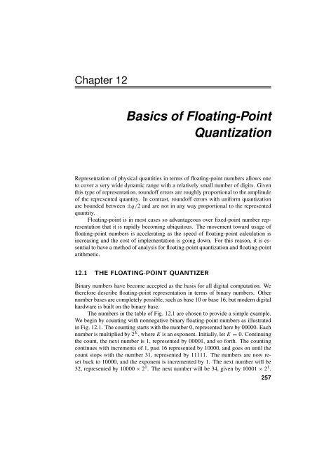
Chapter 12Basics of Floating-PointQuantizationRepresentation of physical quantities in terms of floating-point numbers allows oneto cover a very wide dynamic range with a relatively small number of digits. Giventhis type of representation, roundoff errors are roughly proportional to the amplitudeof the represented quantity. In contrast, roundoff errors with uniform quantizationare bounded between ±q/2 and are not in any way proportional to the representedquantity.Floating-point is in most cases so advantageous over fixed-point number representationthat it is rapidly becoming ubiquitous. The movement toward usage offloating-point numbers is accelerating as the speed of floating-point calculation isincreasing and the cost of implementation is going down. For this reason, it is essentialto have a method of analysis for floating-point quantization and floating-pointarithmetic.12.1 THE FLOATING-POINT QUANTIZERBinary numbers have become accepted as the basis for all digital computation. Wetherefore describe floating-point representation in terms of binary numbers. Othernumber bases are completely possible, such as base 10 or base 16, but modern digitalhardware is built on the binary base.The numbers in the table of Fig. 12.1 are chosen to provide a simple example.We begin by counting with nonnegative binary floating-point numbers as illustratedin Fig. 12.1. The counting starts with the number 0, represented here by 00000. Eachnumber is multiplied by 2 E ,whereE is an exponent. Initially, let E = 0. Continuingthe count, the next number is 1, represented by 00001, and so forth. The countingcontinues with increments of 1, past 16 represented by 10000, and goes on until thecount stops with the number 31, represented by 11111. The numbers are now resetback to 10000, and the exponent is incremented by 1. The next number will be32, represented by 10000 × 2 1 . The next number will be 34, given by 10001 × 2 1 .257

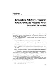
258 12 Basics of Floating-Point QuantizationMantissa0 0 0 0 0 01 0 0 0 0 12 0 0 0 1 03 0 0 0 1 14 0 0 1 0 05 0 0 1 0 16 0 0 1 1 07 0 0 1 1 18 0 1 0 0 09 0 1 0 0 110 0 1 0 1 011 0 1 0 1 112 0 1 1 0 013 0 1 1 0 114 0 1 1 1 015 0 1 1 1 116 −→ 1 0 0 0 017 1 0 0 0 118 1 0 0 1 019 1 0 0 1 120 1 0 1 0 021 1 0 1 0 122 1 0 1 1 023 1 0 1 1 124 1 1 0 0 025 1 1 0 0 126 1 1 0 1 027 1 1 0 1 128 1 1 1 0 029 1 1 1 0 130 1 1 1 1 031 ←− 1 1 1 1 1⎫⎪⎬×2 E⎪⎭Figure 12.1 Counting with binary floating-point numbers with 5-bit mantissa. No sign bitis included here.

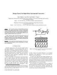
12.1 The Floating-Point Quantizer 259xQx ′FLFigure 12.2 A floating-point quantizer.This will continue with increments of 2 until the number 62 is reached, representedby 11111 × 2 1 . The numbers are again re-set back to 10000, and the exponent isincremented again. The next number will be 64, given by 10000 × 2 2 . And soforth. By counting, we have defined the allowed numbers on the number scale. Eachnumber consists of a mantissa (see page 343) multiplied by 2 raised to a power givenby the exponent E.The counting process illustrated in Fig. 12.1 is done with binary numbers having5-bit mantissas. The counting begins with binary 00000 with E = 0 and goes upto 11111, then the numbers are recycled back to 10000, and with E = 1, the countingresumes up to 11111, then the numbers are recycled back to 10000 again withE = 2, and the counting proceeds.A floating-point quantizer is represented in Fig. 12.2. 1 The input to this quantizeris x, a variable that is generally continuous in amplitude. The output of thisquantizer is x ′ , a variable that is discrete in amplitude and that can only take on valuesin accord with a floating-point number scale. The input–output relation for thisquantizer is a staircase function that does not have uniform steps.Figure 12.3 illustrates the input–output relation for a floating-point quantizerwith a 3-bit mantissa. The input physical quantity is x. Its floating-point representationis x ′ . The smallest step size is q. With a 3-bit mantissa, four steps are takenfor each cycle, except for eight steps taken for the first cycle starting at the origin.The spacings of the cycles are determined by the choice of a parameter . A generalrelation between and q, defining , is given by Eq. (12.1): = △ 2 p q , (12.1)where p is the number of bits of the mantissa. With a 3-bit mantissa, = 8q.Figure 12.3 is helpful in gaining an understanding of relation (12.1). Note that afterthe first cycle, the spacing of the cycles and the step sizes vary by a factor of 2 fromcycle to cycle.1 The basic ideas and figures of the next sections were first published in, and are taken with permissionfrom Widrow, B., Kollár, I. and Liu, M.-C., ”Statistical theory of quantization,” IEEE Transactionson Instrumentation and Measurement 45(6): 35361. c○1995 IEEE.

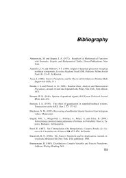
260 12 Basics of Floating-Point Quantization4x ′2Average gain = 1x−4 −2 − 2 4−−22qx ′q−4− 3q 2 − q 2q2−q3q2x−2qFigure 12.3 Input–output staircase function for a floating-point quantizer with a 3-bit mantissa.x xQ ′InputFLOutput− +ν FLFigure 12.4 Floating-point quantization noise.12.2 FLOATING-POINT QUANTIZATION NOISEThe roundoff noise of the floating-point quantizer ν FL is the difference between thequantizer output and input:ν FL = x ′ − x . (12.2)Figure 12.4 illustrates the relationships between x, x ′ ,andν FL .

12.3 An Exact Model of the Floating-Point Quantizer 26112108f νFL6420−2 −1.5 −1 −0.5 0 0.5 1 1.5ν FL2Figure 12.5 The PDF of floating-point quantization noise with a zero-mean Gaussian input,σ x = 32, and with a 2-bit mantissa.The PDF of the quantization noise can be obtained by slicing and stacking thePDF of x, as was done for the uniform quantizer and illustrated in Fig. 5.2. Becausethe staircase steps are not uniform, the PDF of the quantization noise is not uniform.It has a pyramidal shape.With a zero-mean Gaussian input with σ x = 32, and with a mantissa havingjust two bits, the quantization noise PDF has been calculated. It is plotted inFig. 12.5. The shape of this PDF is typical. The narrow segments near the top ofthe pyramid are caused by the occurrence of values of x that are small in magnitude(small quantization step sizes), while the wide segments near the bottom of the pyramidare caused by the occurrence of values of x that are large in magnitude (largequantization step sizes).The shape of the PDF of floating-point quantization noise resembles the silhouetteof a big-city “skyscraper” like the famous Empire State Building of New YorkCity. We have called functions like that of Fig. 12.5 “skyscraper PDFs”. Mathematicalmethods will be developed next to analyze floating-point quantization noise, tofind its mean and variance, and the correlation coefficient between this noise and theinput x.12.3 AN EXACT MODEL OF THE FLOATING-POINTQUANTIZERA floating-point quantizer of the type shown in Fig. 12.3 can be modeled exactly as acascade of a nonlinear function (a “compressor”) followed by a uniform quantizer (a“hidden” quantizer) followed by an inverse nonlinear function (an “expander”). The

262 12 Basics of Floating-Point Quantizationx yy ′x ′CompressorExpanderQNonlinearfunctionUniform quantizer(“Hidden quantizer”)(a)Inversenonlinearfunctionx x ′CompressorExpanderQy− +νy ′− +ν FL(b)Figure 12.6 A model of a floating-point quantizer: (a) block diagram; (b) definition ofquantization noises.overall idea is illustrated in Fig. 12.6(a). A similar idea is often used to representcompression and expansion in a data compression system (see e.g. Gersho and Gray(1992), CCITT (1984)).The input–output characteristic of the compressor (y vs. x) is shown in Fig. 12.7,and the input–output characteristic of the expander (x ′ vs. y ′ ) is shown in Fig. 12.8.The hidden quantizer is conventional, having a uniform-staircase input–output characteristic(y ′ vs. y). Its quantization step size is q, and its quantization noise isν = y ′ − y . (12.3)Figure 12.6(b) is a diagram showing the sources of ν FL and ν. An expression for theinput–output characteristic of the compressor is

12.3 An Exact Model of the Floating-Point Quantizer 263y = x,if − ≤ x ≤ y = 1 2 x + 1 2, if ≤ x ≤ 2y = 1 2 x − 1 2 , if − 2 ≤ x ≤−y = 1 4x + , if 2 ≤ x ≤ 4y = 1 4 x − , if − 4 ≤ x ≤−2.y = 1 x + k 2 k 2 , if 2k−1 ≤ x ≤ 2 k y = 1 x − k 2 k 2 , if − 2k ≤ x ≤−2 k−1 ory = 1 x + sign(x) · k22 , if k 2k−1 ≤|x| ≤2 k ,where k is a nonnegative integer. This is a piecewise-linear characteristic.An expression for the input–output characteristic of the expander isx ′ = y ′ ,if − ≤ y ′ ≤ x ′ = 2(y ′ − 0.5), if ≤ y ′ ≤ 1.5x ′ = 2(y ′ − 0.5), if − 1.5 ≤ y ′ ≤−x ′ = 4(y ′ − ), if 1.5 ≤ y ′ ≤ 2x ′ = 4(y ′ + ), if − 2 ≤ y ′ ≤−1.5.x ′ = 2 k (y ′ − k 2 ), if k+12 ≤ y′ ≤ k+2x ′ = 2 k (y ′ + k 22 ), if −k+22 ≤ y′ ≤− k+12 orx ′ = 2 k (y ′ − sign(y) · k2 ), if k+12 ≤|y′ |≤ k+2(12.4)2 , (12.5)where k is a nonnegative integer. This characteristic is also piecewise linear.One should realize that the compressor and expander characteristics describedabove are universal and are applicable for any choice of mantissa size.The compressor and expander characteristics of Figs. 12.7 and 12.8 are drawnto scale. Fig. 12.9 shows the characteristic (y ′ vs. y) of the hidden quantizer drawnto the same scale, assuming a mantissa of 2 bits. For this case, = 4q.If only the compressor and expander were cascaded, the result would be a perfectgain of unity since they are inverses of each other. If the compressor is cascadedwith the hidden quantizer of Fig. 12.9 and then cascaded with the expander, all inaccord with the diagram of Fig. 12.6, the result is a floating-point quantizer. The oneillustrated in Fig. 12.10 has a 2-bit mantissa.The cascaded model of the floating-point quantizer shown in Fig. 12.6 becomesvery useful when the quantization noise of the hidden quantizer has the properties of

264 12 Basics of Floating-Point Quantization4321y/0−1−2−3−4−4 −3 −2 −1 0 1 2 3 4x/Figure 12.7 The compressor’s input–output characteristic.4321x ′ /0−1−2−3−4−4 −3 −2 −1 0 1 2 3 4y ′ /Figure 12.8 The expander’s input–output characteristic.

12.3 An Exact Model of the Floating-Point Quantizer 2654321y ′ /0−1−2−3−4−4 −3 −2 −1 0 1 2 3 4y/Figure 12.9 The uniform “hidden quantizer.” The mantissa has 2 bits.4321x ′ /0−1−2−3−4−4 −3 −2 −1 0 1 2 3 4x/Figure 12.10 A floating-point quantizer with a 2-bit mantissa.

266 12 Basics of Floating-Point QuantizationPQN. This would happen if QT I or QT II were satisfied at the input y of the hiddenquantizer. Testing for the satisfaction of these quantizing theorems is complicatedby the nonlinearity of the compressor. If x were a Gaussian input to the floatingpointquantizer, the input to the hidden quantizer would be x mapped through thecompressor. The result would be a non-Gaussian input to the hidden quantizer.In practice, inputs to the hidden quantizer almost never perfectly meet the conditionsfor satisfaction of a quantizing theorem. On the other hand, these inputsalmost always satisfy these conditions approximately. The quantization noise ν introducedby the hidden quantizer is generally very close to uniform and very close tobeing uncorrelated with its input y. The PDF of y is usually sliced up so finely thatthe hidden quantizer produces noise having properties like PQN.12.4 HOW GOOD IS THE PQN MODEL FOR THE HIDDENQUANTIZER?In previous chapters where uniform quantization was studied, it was possible to defineproperties of the input CF that would be necessary and sufficient for the satisfactionof a quantizing theorem, such as QT II. Even if these conditions were notobtained, as for example with a Gaussian input, it was possible to determine the errorsthat would exist in moment prediction when using the PQN model. These errorswould almost always be very small.For floating-point quantization, the same kind of calculations for the hiddenquantizer could in principle be made, but the mathematics would be far more difficultbecause of the action of the compressor on the input signal x. The distortion of thecompressor almost never simplifies the CF of the input x nor makes it easy to test forthe satisfaction of a quantizing theorem.To determine the statistical properties of ν, the PDF of the input x can bemapped through the piecewise-linear compressor characteristic to obtain the PDFof y. In turn, y is quantized by the hidden quantizer, and the quantization noise νcan be tested for similarity to PQN. The PDF of ν can be determined directly fromthe PDF of y, or it could be obtained by Monte Carlo methods by applying randomx inputs into the compressor and observing corresponding values of y and ν. Themoments of ν can be determined, and so can the covariance between ν and y. ForthePQN model to be usable, the covariance of ν and y should be close to zero, less thana few percent, the PDF of ν should be almost uniform between ±q/2, and the meanof ν should be close to zero while the mean square of ν should be close to q 2 /12.In many cases with x being Gaussian, the PDF of the compressor output y canbe very “ugly.” Examples are shown in Figs. 12.11(a)–12.14(a). These representcases where the input x is Gaussian with various mean values and various ratios ofσ x /. With mantissas of 4 bits or more, these ugly inputs to the hidden quantizercause it to produce quantization noise which behaves remarkably like PQN. Thisis difficult to prove analytically, but confirming results from slicing and stacking

12.4 How Good is the PQN Model for the Hidden Quantizer? 2670.250.200.15f y (y)0.100.050−6 −5 −4 −3 −2 −1(a)f ν (ν)1/q0 1 2 3 4 5 6y/f ν (ν)1/qq = 16q =256(b)−q/2 q/2ν(c)−q/2 q/2νFigure 12.11 PDF of compressor output and of hidden quantization noise when x is zeromeanGaussian with σ x = 50: (a)f y (y); (b)f ν (ν) for p = 4(q = /16); (c) f ν (ν) forp = 8(q = /256).these PDFs are very convincing. Similar techniques have been used with these PDFsto calculate correlation coefficients between ν and y. The noise ν turns out to beessentially uniform, and the correlation coefficient turns out to be essentially zero.Consider the ugly PDF of y shown in Fig. 12.11(a), f y (y). The horizontal scalegoes over a range of ±5. If we choose a mantissa of 4 bits, the horizontal scale willcover the range ±80q. If we choose a mantissa of 8 bits, q will be much smaller andthe horizontal scale will cover the range ±1280q. With the 4-bit mantissa, slicing andstacking this PDF to obtain the PDF of ν, we obtain the result shown in Fig. 12.11(b).From the PDF of ν, we obtain a mean value of 1.048 · 10 −6 q, and a mean square of0.9996q 2 /12. The correlation coefficient between ν and y is (1.02 · 10 −3 ). Withan 8-bit mantissa, f ν (ν) shown in Fig. 12.11c is even more uniform, giving a meanvalue for ν of −9.448 · 10 −9 q, and a mean square of 1.0001q 2 /12. The correlation

268 12 Basics of Floating-Point Quantization0.50.4f y (y)0.30.20.10−2 −1.5 −1 −0.5(a)f ν (ν)1/q0 0.5 1 1.5 2y/f ν (ν)1/qq = 16q =256(b)−q/2 q/2ν(c)−q/2 q/2νFigure 12.12 PDF of compressor output and of hidden quantization noise when xis Gaussian with σ x = /2 andμ x = σ x : (a) f y (y); (b) f ν (ν) for 4-bit mantissas,(q = /16); (c) f ν (ν) for 8-bit mantissas, (q = /256).

12.4 How Good is the PQN Model for the Hidden Quantizer? 2690.50.4f y (y)0.30.20.10−6 −5 −4 −3 −2 −1(a)f ν (ν)1/q0 1 2 3 4 5 6y/f ν (ν)1/qq = 16q =256(b)−q/2 q/2ν(c)−q/2 q/2νFigure 12.13 PDF of compressor output and of hidden quantization noise when xis Gaussian with σ x = 50 and μ x = σ x : (a) f y (y); (b) f ν (ν) for 4-bit mantissas,(q = /16); (c) f ν (ν) for 8-bit mantissas, (q = /256).

270 12 Basics of Floating-Point Quantizationf y (y)43.532.521.510.50 5 5.25 5.5 5.75 6(a)y/f ν (ν)f ν (ν)1/q1/qq = 16q =256(b)−q/2 q/2ν(c)−q/2 q/2νFigure 12.14 PDF of compressor output and of hidden quantization noise when x isGaussian with σ x = 50 and μ x = 10σ x = 500: (a)f y (y); (b)f ν (ν) for 4-bit mantissas,(q = /16); (c) f ν (ν) for 8-bit mantissas, (q = /256).

12.4 How Good is the PQN Model for the Hidden Quantizer? 271TABLE 12.1 Properties of the hidden quantization noise ν for Gaussian input(a) p = 4 E{ν}/q E{ν 2 }/(q 2 /12) ρ y,νμ x = 0, σ x = 50 0.0002 0.9997 0.0140μ x = σ x ,σ x = 0.5 −0.0015 0.9998 −0.0069μ x = σ x ,σ x = 50 −0.0019 0.9994 −0.0089μ x = σ x ,σ x = 500 −0.0023 0.9987 −0.0077(b) p = 8 E{ν}/q E{ν 2 }/(q 2 /12) ρ y,νμ x = 0, σ x = 50 4.25 · 10 −5 0.9995 8.68 · 10 −4μ x = σ x ,σ x = 0.5 −2.24 · 10 −4 1.0005 −2.35 · 10 −4μ x = σ x ,σ x = 50 −3.72 · 10 −4 0.9997 −1.30 · 10 −3μ x = σ x ,σ x = 500 −1.92 · 10 −4 0.9985 −8.77 · 10 −4coefficient between ν and y is (2.8 · 10 −4 ). With a mantissa of four bits or more, thenoise ν behaves very much like PQN.This process was repeated for the ugly PDFs of Figs. 12.12(a), 12.13(a), and12.14(a). The corresponding PDFs of the quantization noise of the hidden quantizerare shown in Figs. 12.12(b), 12.13(b), and 12.14(b). With a 4-bit mantissa,Table 12.1(a) lists the values of mean and mean square of ν, and correlation coefficientbetween ν and y for all the cases. With an 8-bit mantissa, the correspondingmoments are listed in Table 12.1(b).Similar tests have been made with uniformly distributed inputs, with triangularlydistributed inputs, and with sinusoidal inputs. Input means ranged from zero toone standard deviation. The moments of Tables 12.1(a),(b) are typical for Gaussianinputs, but similar results are obtained with other forms of inputs.For every single test case, the input x had a PDF that extended over at leastseveral multiples of . With a mantissa of 8 bits or more, the noise of the hiddenquantizer had a mean of almost zero, a mean square of almost q 2 /12, and a correlationcoefficient with the quantizer input of almost zero.The PQN model works so well that we assume that it is true as long as themantissa has 8 or more bits and the PDF of x covers at least several -quanta of thefloating-point quantizer. It should be noted that the single precision IEEE standard(see Section 13.8) calls for a mantissa with 24 bits. When working with this standard,the PQN model will work exceedingly well almost everywhere.

272 12 Basics of Floating-Point Quantization12.5 ANALYSIS OF FLOATING-POINT QUANTIZATIONNOISEWe will use the model of the floating-point quantizer shown in Fig. 12.6 to determinethe statistical properties of ν FL . We will derive its mean, its mean square, and itscorrelation coefficient with input x.The hidden quantizer injects noise into y, resulting in y ′ , which propagatesthrough the expander to make x ′ . Thus, the noise of the hidden quantizer propagatesthrough the nonlinear expander into x ′ . The noise in x ′ is ν FL .Assume that the noise ν of the hidden quantizer is small compared to y. Thenν is a small increment to y. This causes an increment ν FL at the expander output.Accordingly,( dx′ν FL = ν . (12.6)dy ′ )yThe derivative is a function of y. This is because the increment ν is added to y, soyis the nominal point where the derivative should be taken.Since the PQN model was found to work so well for so many cases with regardto the behavior of the hidden quantizer, we will make the assumption that the conditionsfor PQN are indeed satisfied for the hidden quantizer. This greatly simplifiesthe statistical analysis of ν FL .Expression (12.6) can be used in the following way to find the crosscorrelationbetween ν FL and input x.{ ( }dx′E{ν FL x}=E ν · · x= E {ν} Edy ′ )y{ (dx′dy ′ )y= 0 . (12.7)When deriving this result, it was possible to factor the expectation into a productof expectations because, from the point of view of moments, ν( behaves as if it isindependent of y and independent of any function of y, suchas dx ′dy)y ′ and x. Sincethe expected value of ν is zero, the crosscorrelation turns out to be zero.Expression (12.6) can also be used to find the mean of ν FL . Accordingly,{ ( }dx′E{ν FL }=E ν ·= E{ν}Edy ′ )y{ (dx′dy ′ )y· x}}= 0 . (12.8)

12.5 Analysis of Floating-Point Quantization Noise 273So the mean of ν FL is zero, and the crosscorrelation between ν FL and x is zero. Bothresults are consequences of the hidden quantizer behaving in accord with the PQNmodel.Our next(objective is the determination of E{ν 2 FL}. We will need to find an expressionfor dx ′dy)y ′ in order to obtain quantitative results. By inspection of Figs. 12.7and 12.8, which show the characteristics of the compressor and the expander, we determinethatdx ′dy ′ = 1 when 0.5

274 12 Basics of Floating-Point Quantization3.5log 2( x)+ 0.52.51.50.5−0.50 2 3 4 5 6 7 8(a)( ( x) )Q 1 log 2 + 0.54x32100 2 3 4 5 6 7 8(b)xFigure 12.15 Approximate and ( exact exponent characteristics: )(a) logarithmic approximation;(b) exact expression, Q 1 log 2 (x/) + 0.5 vs. x.

12.5 Analysis of Floating-Point Quantization Noise 275Referring back to (12.9), it is apparent that for positive values of x, the derivativecan be represented in terms of the new function as( x) )dx′= 2 Q 1((log 2 + 0.5 , x >/2 . (12.11)dy ′ )xFor negative values of x, the derivative is((( −xdx′ Q 1 log 2= 2 dy ′ )xAnother way to write this is( dx′dy ′ )x((|x|Q 1 log 2= 2 ) )+ 0.5) )+ 0.5These are exact expressions for the derivative.From Eqs. (12.13) and Eq. (12.6), we obtain ν FL as, x < −/2 . (12.12), |x| >/2 . (12.13)(( ) )|x|Q 1 log 2 + 0.5ν FL = ν · 2 , |x| >/2 . (12.14)One should note that the value of would generally be much smaller than the valueof x. At the input level of |x|

276 12 Basics of Floating-Point Quantization= √ 2ν · |x| 2ν EXP. (12.17)The mean square of ν FL can be obtained from this.{ }E{ν 2 }=2E FLν 2 x2 2 22ν EXP{ x= 2E{ν 2 2}}E. (12.18) 2 22ν EXPThe factorization is permissible because by assumption ν behaves as PQN. The noiseν EXP is related to x, but since ν EXP is bounded, it is possible to upper and lower boundE{ν 2 } even without knowledge of the relation between ν FL EXP and x. The bounds areE{ν 2 }E{ x2 2 }≤E{ν2 FL }≤4E{ν2 }E{ x2 2 }. (12.19)). From the point of view of moments, ν EXP will behave as if it isThese bounds hold without exception as long as the PQN model applies for the hiddenquantizer.If, in addition to this, the PQN model applies to the quantized exponent inEq. (12.15), then a precise value for E{ν 2 } can be obtained. With PQN, ν FL EXP willhave zero mean, a mean square of 1/12, a mean fourth of 1/80, and will be uncorre-(lated with log |x|2 independent of x and any function of x. From Eq. (12.17),ν FL = √ 2 · ν · |x| 2ν EXP= √ 2 · ν · |x| eν EXP ln 2 . (12.20)From this, we can obtain E{ν 2 }: FL{E{ν 2 }=2E FLν 2 x2 2 e2ν EXP ln 2 }= 2E{ν 2 x2 ( 2 1 + 2ν EXP ln 2 + 1 2! (2ν EXP ln 2) 2 + 1 3! (2ν EXP ln 2) 3+ 1 ) }4! (2ν EXP ln 2) 4 +···{ x= E{ν 2 2} {}E 2 E 2 + 4ν EXP ln 2 + 4ν 2 (ln EXP 2)2 + 8 3 ν3 EXP(ln 2)3+ 4 }3 ν4 (ln EXP 2)4 +··· . (12.21)Since the odd moments of ν EXP are all zero,{ xE{ν 2 2}(FL }=E{ν2 }E 2 2 + 4( 112 )(ln 2)2 + ( 4 3 )( 1)80 )(ln 2)4 +···

12.5 Analysis of Floating-Point Quantization Noise 277{ x= 2.16 · E{ν 2 2}}E 2 . (12.22)This falls about half way between the lower and upper bounds.A more useful form of this expression can be obtained by substituting the following,E{ν 2 }= q212 , and q = 2−p . (12.23)The result is a very important one:E{ν 2 }=0.180 · FL 2−2p · E{x 2 } . (12.24)Example 12.1 Roundoff noise when multiplying two floating-point numbersLet us assume that two numbers: 1.34 · 10 −3 and 4.2 are multiplied using IEEEdouble precision arithmetic. The exact value of the roundoff error could be determinedby using the result of more precise calculation (with p > 53) as areference. However, this is usually not available.The mean square of the roundoff noise can be easily determined using Eq. (12.24),without the need of reference calculations. The product equals 5.63·10 −3 . Whentwo numbers of magnitudes similar as above are multiplied, the roundoff noisewill have a mean square of E{ν 2 }≈0.180 · FL 2−2p · 3.2 · 10 −5 . Although wecannot determine the precise roundoff error value for the given case, we can giveits expected magnitude.Example 12.2 Roundoff noise in 2nd-order IIR filtering with floating pointLet us assume one evaluates the recursive formulay(n) =−a(1)y(n − 1) − a(2)y(n − 2) + b(1)x(n − 1).When the operations (multiplications and additions) are executed in natural order,all with precision p, the following sources of arithmetic roundoff can beenumerated:1. roundoff after the multiplication a(1)y(n − 1):var{ν FL1 }≈0.180 · 2 −2p · a(1) 2 · var{y},2. roundoff after the storage of −a(1)y(n − 1):var{ν FL2 }=0, since if the product in item 1 is rounded, the quantity to bestored is already quantized,3. roundoff after the multiplication a(2)y(n − 2):var{ν FL3 }≈0.180 · 2 −2p · a(2) 2 · var{y},4. roundoff after the addition −a(1)y(n − 1) − a(2)y(n − 2):var{ν FL4 }≈0.180 · 2 −2p ( a(1) 2 · var{y}+a(2) 2 · var{y}+2a(1)a(2) · C yy (1) ) ,5. roundoff after the storage of −a(1)y(n − 1) − a(2)y(n − 2):var{ν FL5 }=0, since if the product in item 4 is rounded, the quantity to bestored is already quantized,

278 12 Basics of Floating-Point Quantization6. roundoff after the multiplication b(1)x(n − 1):var{ν FL6 }≈0.180 · 2 −2p · b(1) 2 · var{x},7. roundoff after the last addition:var{ν FL7 }≈0.180 · 2 −2p · var{y},8. roundoff after the storage of the result to y(n):var{ν FL8 }=0, since if the sum in item 7 is rounded, the quantity to bestored is already quantized.These variances need to be added to obtain the total variance of the arithmeticroundoff noise injected to y in each step.The total noise variance in y can be determined then by adding the effect of eachinjected noise. This can be done using the response to an impulse injected toy(0): ifthisisgivenbyh yy (0), h yy (1),..., including the unit impulse itself attime 0, the variance of the total roundoff noise can be calculated by multiplying∑the above variance of the injected noise by ∞ h 2 yy (n).For all these calculations, one also needs to determine the variance of y, and theone-step covariance C yy (1).If x is sinusoidal with amplitude A, y is also sinusoidal with an amplitude determinedby the transfer function: var{y} =|H( f 1 )| 2 var{x} =|H( f 1 )| 2 A 2 /2.C yy (1) ≈ var{y} for low-frequency sinusoidal input.∑If x is zero-mean white noise, var{y} =var{x} ∞ h 2 (n), with h(n) being then=0∑impulse response from x to y. The covariance is about var{x} ∞ h(n)h(n + 1).Numerically, let us use single precision (p = 24), and let a(1) =−0.9, a(2) =0.5, and b(1) = 0.2, and let the input signal be a sine wave with unit power(A 2 /2 = 1), and frequency f 1 = 0.015 f s . With these, H( f 1 ) = 0.33, andvar{y} =0.11, and the covariance C yy (1) approximately equals var{y}. Evaluatingthe variance of the floating-point noise,8∑var{ν FL }= var{ν FLn }≈1.83 · 10 −16 . (12.25)n=1The use of extended-precision accumulator and of multiply-and-add operationIn many modern processors, an accumulator is used with extended precisionp acc , and multiply-and-add operation (see page 374) can be applied. In thiscase, multiplication is usually executed without roundoff, and additions are notfollowed by extra storage, therefore roundoff happens only for certain items (but,in addition to the above, var{ν FL2 } ̸= 0, since ν FL1 = 0). The total variance of y,caused by arithmetic roundoff, isvar inj = var{ν FL2 }+var{ν FL4 }+var{ν FL7 }+var{ν FL8 }= 0.180 · 2 −2p acc· a(1) 2 var{y}n=0n=0

12.5 Analysis of Floating-Point Quantization Noise 279()+ 0.180 · 2 −2p acca(1) 2 var{y}+a(2) 2 var{y}+2a(1)a(2)C yy (1)+ 0.180 · 2 −2p acc· var{y}+ 0.180 · 2 −2p · var{y} . (12.26)In this expression, usually the last term dominates. With the numerical data,var{ν FL-ext} ≈7.1 · 10 −17 .Making the same substitution in Eq. (12.19), the bounds are112 · 2−2p · E{x 2 }≤E{ν 2 FL }≤1 3 · 2−2p · E{x 2 } . (12.27)The signal-to-noise ratio for the floating-point quantizer is defined asSNR = △ E{x2 }E{νFL} 2 . (12.28)If both ν and ν EXP obey PQN models, then Eq. (12.24) can be used to obtain the SNR.The result is:SNR = 5.55 · 2 2p . (12.29)This is the ratio of signal power to quantization noise power. Expressed in dB, theSNR isSNR, dB ≈ 10 log((5.55)2 2p)= 7.44 + 6.02p . (12.30)If only ν obeys a PQN model, then Eq. (12.27) can be used to bound the SNR:12 · 2 2p ≥ SNR ≥ 3 · 2 2p . (12.31)This can be expressed in dB as:4.77 + 6.02p ≤ SNR, dB ≤ 10.79 + 6.02p . (12.32)From relations Eq. (12.29) and Eq. (12.31), it is clear that the SNR improves as thenumber of bits in the mantissa is increased. It is also clear that for the floatingpointquantizer, the SNR does not depend on E{x 2 } (as long as ν and ν EXP act likePQN). The quantization noise power is proportional to E{x 2 }. This is a very differentsituation from that of the uniform quantizer, where SNR increases in proportion toE{x 2 } since the quantization noise power is constant at q 2 /12.When ν satisfies a PQN model, ν FL is uncorrelated with x. The floating-pointquantizer can be replaced for purposes of least-squares analysis by an additive independentnoise having a mean of zero and a mean square bounded by (12.27). If in ad-

280 12 Basics of Floating-Point Quantizationdition ν EXP satisfies a PQN model, the mean square of ν will be given by Eq. (12.24).Section 12.6 discusses the question about ν EXP satisfying a PQN model. This doeshappen in a surprising number of cases. But when PQN fails for ν EXP , we cannotobtain E{ν 2 FL} from Eq. (12.24), but we can get bounds on it from (12.27).12.6 HOW GOOD IS THE PQN MODEL FOR THE EXPONENTQUANTIZER?The PQN model for the hidden quantizer turns out to be a very good one when themantissa has 8 bits or more, and: (a) the dynamic range of x extends over at leastseveral times , (b) for the Gaussian case, σ x is at least as big as /2. This modelworks over a very wide range of conditions encountered in practice. Unfortunately,the range of conditions where a PQN model would work for the exponent quantizeris much more restricted. In this section, we will explore the issue.12.6.1 Gaussian InputThe simplest and most important case is that of the Gaussian input. Let the input xbe Gaussian with variance σx 2, and with a mean μ x that could vary between zero andsome large multiple of σ x , say 20σ x . Fig. 12.16 shows calculated plots of the PDF ofν EXP for various values of μ x . This PDF is almost perfectly uniform between ± 1 2 forμ x = 0, 2σ x ,and3σ x . For higher values of μ x , deviations from uniformity are seen.The covariance of ν EXP and x, shown in Fig. 12.17, is essentially zero forμ x = 0, 2σ x ,and3σ x . But for higher values of μ x , significant correlation developsbetween ν EXP and x. Thus, the PQN model for the exponent quantizer appearsto be intact for a range of input means from zero to 3σ x . Beyond that, this PQNmodel appears to break down. The reason for this is that the input to the exponentquantizer is the variable |x|/ going through the logarithm function. The greater themean of x, the more the logarithm is saturated and the more the dynamic range ofthe quantizer input is compressed.The point of breakdown of the PQN model for the exponent quantizer is notdependent on the size of the mantissa, but is dependent only on the ratios of σ x to and σ x to μ x .When the PQN model for the exponent quantizer is applicable, the PQN modelfor the hidden quantizer will always be applicable. The reason for this is that theinput to both quantizers is of the form log 2 (x), but for the exponent quantizer xis divided by , making its effective quantization step size , and for the hiddenquantizer, the input is not divided by anything and so its quantization step size is q.The quantization step of the exponent quantizer is therefore coarser than that of thehidden quantizer by the factorq = 2p . (12.33)

12.6 How Good is the PQN Model for the Exponent Quantizer? 281f νEXP (ν EXP )f νEXP (ν EXP )11−1/2 1/2(a)f νEXP (ν EXP )ν EXP−1/2 1/2(b)f νEXP (ν EXP )ν EXP11−1/2 1/2(c)ν EXP−1/2 1/2(d)f νEXP (ν EXP )ν EXPf νEXP (ν EXP )11−1/2 1/2(e)ν EXP−1/2 1/2(f)ν EXPFigure 12.16 PDFs of noise of exponent quantizer, for Gaussian input x, with σ x = 512:(a) μ x = 0; (b) μ x = σ x ;(c)μ x = 2σ x ;(d)μ x = 3σ x ;(e)μ x = 5σ x ; (f) μ x = 9σ x .

282 12 Basics of Floating-Point Quantization1.00.80.60.40.2ρ x,νEXP0−0.2−0.4−0.6−0.8−1.0 0 2 4 6 8 10 12 14 16 18 20μ x /σ xFigure 12.17 Correlation coefficient between ν EXP and x versus μ x /σ x , for Gaussianinput x with σ x = 512.With an 8-bit mantissa, this ratio would be 256. So if the conditions for PQN are metfor the exponent quantizer, they are easily met for the hidden quantizer.For the Gaussian input case, the PQN model for the exponent quantizer worksto within a close approximation for 0 ≤ μ x < 3σ x . The correlation coefficient betweenν EXP and x, plotted versus μ x /σ x in Fig. 12.17, indicates very small correlationwith μ x in this range. One would therefore expect formula (12.24) for E{ν 2 FL} to bevery accurate in these circumstances, and it is.Eq. (12.24) may be rewritten in the following way:( E{ν0.180 = 2 2p 2} )FLE{x 2 . (12.34)}This form of (12.24) suggests a new definition:⎛⎞normalizedfloating-point( △ E{ν⎜⎟ = 2 2p 2} )FL⎝ quantization ⎠ E{x 2 . (12.35)}noise powerThe normalized floating-point quantization noise power (NFPQNP) will be equal tothe “magic number” 0.180 when a PQN model applies to the exponent quantizerand, of course, another PQN model applies to the hidden quantizer. Otherwise theNFPQNP will not be exactly equal to 0.180, but it will be bounded. From Eq. (12.27),

12.6 How Good is the PQN Model for the Exponent Quantizer? 2830.350.30Upper bound0.25NFPQNP0.200.150.1800.10Lower bound0.050 2 4 6 8 10 12 14 16 18 20μ x /σ xFigure 12.18 Normalized floating-point quantization noise power (NFPQNP) versusμ x /σ x , for Gaussian input x with σ x = 512 and 8-bit mantissas.⎛⎞normalized112 ≤ floating-point⎜⎟⎝ quantization ⎠ ≤ 1 3 . (12.36)noise powerThese bounds rely on the applicability of a PQN model for the hidden quantizer.For the Gaussian input case, the NFPQNP is plotted versus the ratio of inputmean to input standard deviation in Fig. 12.18. The value of NFPQNP is very closeto 0.180 for 0 ≤ (μ x /σ x )

284 12 Basics of Floating-Point Quantization5 × 10 −54 × 10 −53 × 10 −52 × 10 −51 × 10 −5μ νFL /μ x 0−1 × 10 −5−2 × 10 −5−3 × 10 −5−4 × 10 −5−5 × 10 −5 0 2 4 6 8 10 12 14 16 18 20μ x /σ xFigure 12.19 Relative mean of the floating-point noise: μ νFL /μ x versus μ x /σ x ,forGaussian input x, with σ x = 512, and 8-bit mantissas.0.0100.0080.0060.0040.002ρ x,νFL0−0.002−0.004−0.006−0.008−0.010 0 2 4 6 8 10 12 14 16 18 20μ x /σ xFigure 12.20 Correlation coefficient of floating-point quantization noise and input x:ρ νFL ,x versus μ x /σ x , for Gaussian input x, with σ x = 512, and 8-bit mantissas.

12.6 How Good is the PQN Model for the Exponent Quantizer? 2850.0100.0080.0060.0040.002ρ y,ν0−0.002−0.004−0.006−0.008−0.010 0 2 4 6 8 10 12 14 16 18 20μ x /σ xFigure 12.21 Correlation coefficient of the hidden quantization noise and input y: ρ ν,yversus μ x /σ x , for Gaussian input x, with σ x = 512, and 8-bit mantissas.For purposes of analysis, it is clear that the floating-point quantizer can bereplaced by a source of additive independent noise with zero mean and mean squaregiven by Eq. (12.24) or bounded by (12.27).12.6.2 Input with Triangular DistributionA similar set of calculations and plots have been made for an input x having a triangularPDF with variable mean. The results are shown in Figs. 12.23–12.28. Fig. 12.23showsPDFsofν EXP for various mean values of input x. The amplitude range of xis ±A + μ x . The correlation coefficient between ν EXP and x is moderately small for0 ≤ μ x < A, the PDFs of ν EXP are close to uniform in that range, and they becomenon uniform outside this range.Thus, the PQN model works well for the exponent quantizer in the range 0 ≤μ x < A. Outside this range, the PQN model begins to break down. This is confirmedby inspection of the normalized floating-point quantization noise power which hasbeen calculated and plotted in Fig. 12.25.The mean of ν FL is very close to zero. When normalized with respect to themean of x, the relative mean remains less than a few parts per 10 5 over the range ofinput means from 0

286 12 Basics of Floating-Point Quantizationf ν (ν)1/qf ν (ν)1/qq =256q =256−q/2 q/2(a)ν−q/2 q/2(b)νf ν (ν)1/qf ν (ν)1/qq =256q =256−q/2 q/2(c)ν−q/2 q/2(d)νFigure 12.22 Noise PDFs for hidden quantizer, Gaussian input PDF with σ x = 512,and8-bit mantissas, (a) μ x = 0; (b) μ x = 5σ x ;(c) μ x = 14.5σ x ;(d) μ x = 17σ x .12.6.3 Input with Uniform DistributionA more difficult case is that of input x having a uniform PDF. The abrupt cutoffsat the edges of this PDF cause the CF of x to have wide “bandwidth.” A study ofthe floating-point quantizer having an input of variable mean and a uniform PDF hasbeen done, and results are shown in Figs. 12.29–12.35. The width of the uniformPDF is 2A.Fig. 12.29 gives PDFs of the noise of the exponent quantizer for various meanvalues of x. Fig. 12.30 shows the correlation coefficient of ν EXP and input x for μ xin the range 0

12.6 How Good is the PQN Model for the Exponent Quantizer? 287f νEXP (ν EXP )f νEXP (ν EXP )11−1/2 1/2(a)f νEXP (ν EXP )ν EXP−1/2 1/2(b)f νEXP (ν EXP )ν EXP11−1/2 1/2(c)ν EXP−1/2 1/2(d)ν EXPFigure 12.23 PDFs of noise of exponent quantizer, for triangular input PDF, with A =400: (a)μ x = 0; (b) μ x = A; (c) μ x = 2A; (d) μ x = 2.5A.explore this, we plotted the correlation coefficient between the hidden quantizationnoise ν and the hidden quantizer input y. This is shown in Fig. 12.34. The correlationcoefficient is less than 2% until μ x /A ≈ 6. It appears that PQN for the hiddenquantizer is beginning to breakdown when μ x /A becomes greater than 6.PDFs of ν have been plotted to study the break down of PQN, and the results areshown in Fig. 12.35. The PDFs are perfectly uniform or close to uniform, but irregularitiesappear for μ x /A higher than 6. The correlation coefficients ρ ν,y and ρ νFL ,xalso indicate PQN break down for μ x /A greater than 6. By increasing the numberof mantissa bits by a few, these breakdown indicators, which are slight, disappearaltogether.For purposes of moment analysis, the floating-point quantizer can be replacedby a source of additive zero-mean independent noise whose mean square is given byEq. (12.24) or is bounded by (12.27). One must be sure, however, that the mantissahas enough bits to allow the PQN model to apply to the hidden quantizer. Then ν FLis uncorrelated with x, and the quantizer replacement with additive noise is justified.

288 12 Basics of Floating-Point Quantization1.00.80.60.40.2ρ x,νEXP0−0.2−0.4−0.6−0.8−1.00 2 4 6 8 10 12 14 16 18 20μ x /A xFigure 12.24 Correlation coefficient between ν EXP and x versus μ x /A, for triangular inputPDF with A = 400.0.350.30Upper bound0.25NFPQNP0.200.150.1800.10Lower bound0.050 2 4 6 8 10 12 14 16 18 20μ x /AFigure 12.25 Normalized floating-point quantization noise power (NFPQNP) versusμ x /A, for triangular input PDF with A = 400, and 8-bit mantissas.

12.6 How Good is the PQN Model for the Exponent Quantizer? 2895 × 10 −54 × 10 −53 × 10 −52 × 10 −51 × 10 −5μ νFL /μ x 0−1 × 10 −5−2 × 10 −5−3 × 10 −5−4 × 10 −5−5 × 10 −5 0 2 4 6 8 10 12 14 16 18 20μ x /AFigure 12.26 Relative mean of the floating-point noise: μ νFL /μ x versus μ x /A, for triangularinput PDF with A = 400, and 8-bit mantissas.0.0200.0150.0100.005ρ x,νFL0−0.005−0.010−0.015−0.020 0 2 4 6 8 10 12 14 16 18 20μ x /AFigure 12.27 Correlation coefficient of floating-point quantization noise and input x:ρ νFL ,x versus μ x /A, for triangular input PDF with A = 400, and 8-bit mantissas.

290 12 Basics of Floating-Point Quantization0.0200.0150.0100.005ρ y,ν0−0.005−0.010−0.015−0.020 0 2 4 6 8 10 12 14 16 18 20μ x /AFigure 12.28 Correlation coefficient of the hidden quantization noise and input y: ρ ν,yversus μ x /A, for triangular input PDF with A = 500, and 8-bit mantissas.12.6.4 Sinusoidal InputThe PDF of the sinusoidal input, like the uniform PDF, has abrupt cutoff at its edges.Its shape is even worse than that of the uniform PDF from the point of view ofsatisfying conditions for PQN. Results of a study of a floating-point quantizer witha sinusoidal input and a variable mean are shown in Figs. 12.36–12.42. The zero-topeakamplitude of the sinusoidal input is A.Fig. 12.36 gives PDFs of the noise of the exponent quantizer for various meanvalues of x. None of these PDFs suggest PQN conditions for the exponent quantizer,even when μ x = 0. This is testimony to the difficulty of satisfying PQN condition forthe case of the sinusoidal input. Fig. 12.37 shows the correlation coefficient betweenν EXP and input x for various values of the input mean μ x . The correlation coefficientis most often very far from zero, further indicating that PQN conditions are not metfor the exponent quantizer. Accordingly, it will not be possible to get an accuratevalue of E{ν 2 } from Eq. (12.34), but it will be possible to bound FL E{ν2 FL} by using(12.36).Fig. 12.38(a) shows the normalized floating-point quantization noise power fora variety of input mean values. The mantissa has p = 8 bits. As long as PQNis satisfied for the hidden quantizer, the normalized quantization noise power stayswithin the bounds. This seems to be the case. With the mantissa length doubledto p = 16 bits, the normalized floating-point noise power measurements, plotted inFig. 12.38(b), came out the same. PQN is surely satisfied for the hidden quantizerwhen given such a long mantissa. More evidence will follow.

12.6 How Good is the PQN Model for the Exponent Quantizer? 291f νEXP (ν EXP )f νEXP (ν EXP )11−1/2 1/2(a)f νEXP (ν EXP )ν EXP−1/2 1/2(b)f νEXP (ν EXP )ν EXP11−1/2 1/2(c)ν EXP−1/2 1/2(d)ν EXPFigure 12.29 PDFs of noise of exponent quantizer, for uniform input PDF with A =400: (a)μ x = 0; (b) μ x = 1.5A; (c) μ x = 2.5A; (d) μ x = 4A.

292 12 Basics of Floating-Point Quantization1.00.80.60.40.2ρ x,νEXP0−0.2−0.4−0.6−0.8−1.00 2 4 6 8 10 12 14 16 18 20μ x /AFigure 12.30 Correlation coefficient between ν EXP and x versus μ x /A, for uniform inputPDF with A = 400.0.350.30Upper bound0.25NFPQNP0.200.150.1800.10Lower bound0.050 2 4 6 8 10 12 14 16 18 20μ x /AFigure 12.31 Normalized floating-point quantization noise power (NFPQNP) versusμ x /A, for uniform input PDF with A = 400 and 8-bit mantissas.

12.6 How Good is the PQN Model for the Exponent Quantizer? 2931 × 10 −48 × 10 −56 × 10 −54 × 10 −52 × 10 −5μ νFL /μ x 0−2 × 10 −5−4 × 10 −5−6 × 10 −5−8 × 10 −5−1 × 10 −4 0 2 4 6 8 10 12 14 16 18 20μ x /AFigure 12.32 Relative mean of the floating-point noise: μ νFL /μ x versus μ x /A, for uniforminput PDF with A = 400 and 8-bit mantissas.ρ x,νFL0.0200.100.080.060.04−0.02−0.04−0.06−0.08−0.10 0 2 4 6 8 10 12 14 16 18 20μ x /AFigure 12.33 Correlation coefficient of floating-point quantization noise and input x:ρ νFL ,x versus μ x /A, for uniform input PDF with A = 400 and 8-bit mantissas.

294 12 Basics of Floating-Point Quantizationρ y,ν0.0200.100.080.060.04−0.02−0.04−0.06−0.08−0.10 0 2 4 6 8 10 12 14 16 18 20μ x /AFigure 12.34 Correlation coefficient of hidden quantization noise ν and hidden quantizerinput y: ρ ν,y versus μ x /A, for uniform input PDF with A = 400 and 8-bit mantissas.f ν (ν)1/qf ν (ν)1/qq =256q =2568−q/2 q/2(a)ν−q/2 q/2(b)νf ν (ν)1/qf ν (ν)1/qq =256q =256−q/2 q/2(c)ν−q/2 q/2(d)νFigure 12.35 Noise PDFs for hidden quantizer, uniform input PDF with A = 200,8-bitmantissas, (a) μ x = 0; (b) μ x = 10A; (c) μ x = 15A; (d) μ x = 16A.

12.6 How Good is the PQN Model for the Exponent Quantizer? 295f νEXP (ν EXP )f νEXP (ν EXP )11−1/2 1/2(a)ν EXP−1/2 1/2(b)f νEXP (ν EXP )ν EXPf νEXP (ν EXP )1−1/2 1/2(c)ν EXP1−1/2 1/2(d)ν EXPFigure 12.36 PDFs of noise of the exponent quantizer, for sinusoidal input with A =400: (a)μ x = 0; (b) μ x = A; (c)μ x = 2A; (d)μ x = 4A.

296 12 Basics of Floating-Point Quantization1.00.80.60.40.2ρ x,νEXP0−0.2−0.4−0.6−0.8−1.00 2 4 6 8 10 12 14 16 18 20μ x /AFigure 12.37 Correlation coefficient between ν EXP and x versus μ x /A, for sinusoidalinput, A = 400.The relative mean of ν FL with an 8-bit mantissa is plotted in Fig. 12.39(a) for avariety of input mean values. The relative mean is very small, a few parts in 10 000at worst. The mean of ν FL being close to zero is consistent with PQN being satisfiedfor the hidden quantizer. Doubling the length of the mantissa to 16 bits, the relativemean, plotted in Fig. 12.39(b), becomes very very small, a few parts in 10 000 000,for a range of input mean values.Fig. 12.40 shows the correlation coefficient of ν FL and x for various mean valuesof x. Fig. 12.40(a) corresponds to p = 8 bits. The correlation coefficient ishighly variable as μ x is varied, and at worst could be as high as 25%. As such, onecould not replace the floating-point quantizer with a source of additive independentnoise. PQN for the hidden quantizer fails. So the correlation coefficient was reevaluatedwith a 16-bit mantissa, and the result, shown in Fig. 12.40(b), indicates acorresponding worst-case correlation coefficient of the order of 1%. With this mantissa,it seems reasonable that one could replace the floating-point quantizer with asource of additive independent noise. The resulting analysis would be a very goodapproximation to the truth. PQN for the hidden quantizer is a good approximation.Fig. 12.41 shows correlation coefficients between the hidden quantization noiseand the hidden quantizer input for various values of μ x . These figures are verysimilar to Figs. 12.40(a)-(b), respectively. Relationships between ρ νFL ,x and ρ ν,ywill be discussed below.One final check will be made on the PQN hypothesis for the hidden quantizer.Fig. 12.42 shows the PDF of ν for the hidden quantizer for various values of inputmean. These PDFs are not quite uniform, and in some cases they are far from uni-

12.6 How Good is the PQN Model for the Exponent Quantizer? 2970.350.30Upper bound0.25NFPQNP0.200.150.1800.10Lower bound0.050 2 4 6 8 10 12 14 16 18 20(a)μ x /A0.350.30Upper bound0.25NFPQNP0.200.150.1800.10Lower bound0.050 2 4 6 8 10 12 14 16 18 20(b)μ x /AFigure 12.38 Normalized floating-point quantization noise power (NFPQNP) vs. μ x /A,for a sinusoidal input with A = 400: (a) 8-bit mantissa; (b) 16-bit mantissa.

298 12 Basics of Floating-Point Quantization1 × 10 −38 × 10 −46 × 10 −44 × 10 −42 × 10 −4μ νFL /μ x 0−2 × 10 −4−4 × 10 −4−6 × 10 −4−8 × 10 −4−1 × 10 −3 0 2 4 6 8 10 12 14 16 18 20(a)μ x /A1 × 10 −78 × 10 −86 × 10 −84 × 10 −82 × 10 −8μ νFL /μ x 0−2 × 10 −8−4 × 10 −8−6 × 10 −8−8 × 10 −8−1 × 10 −7 0 2 4 6 8 10 12 14 16 18 20(b)μ x /AFigure 12.39 Relative mean of the floating-point noise, ν FL /μ x versus μ x /A, for sinusoidalinput with A = 400: (a) 8-bit mantissa; (b) 16-bit mantissa.

12.6 How Good is the PQN Model for the Exponent Quantizer? 299ρ x,νFL0.0500.250.200.150.10−0.05−0.10−0.15−0.20−0.25 0 2 4 6 8 10 12 14 16 18 20(a)μ x /A0.0100.0080.0060.0040.002ρ x,νFL0−0.002−0.004−0.006−0.008−0.010 0 2 4 6 8 10 12 14 16 18 20(b)μ x /AFigure 12.40 Correlation coefficient of floating-point quantization noise and input x,ρ νFL ,x versus μ x /A for sinusoidal input, with A = 400: (a) 8-bit mantissa; (b) 16-bitmantissa.

300 12 Basics of Floating-Point Quantizationρ y,ν0.0500.250.200.150.10−0.05−0.10−0.15−0.20−0.25 0 2 4 6 8 10 12 14 16 18 20(a)μ x /A0.0100.0080.0060.0040.002ρ y,ν0−0.002−0.004−0.006−0.008−0.010 0 2 4 6 8 10 12 14 16 18 20(b)μ x /AFigure 12.41 Correlation coefficient of hidden quantization noise ν and hidden quantizerinput y, ρ ν,y versus μ x /A for sinusoidal input with A = 400: (a) 8-bit mantissa; (b) 16-bit mantissa.

12.6 How Good is the PQN Model for the Exponent Quantizer? 301f ν (ν)f ν (ν)1/qq =2561/qq =256−q/2 q/2(a)ν−q/2 q/2(b)νf ν (ν)f ν (ν)1/qq =25681/qq =256−q/2 q/2(c)ν−q/2 q/2(d)νFigure 12.42 Noise PDFs for the hidden quantizer, sinusoidal input, A = 400, 8-bitmantissas: (a) μ x = 0; (b) μ x = 1.75A; (c)μ x = 6.5A; (d)μ x = 12A.

302 12 Basics of Floating-Point Quantizationf ν (ν)f ν (ν)1/q1/qq =65536q =65536−q/2 q/2(a)ν−q/2 q/2(b)νf ν (ν)f ν (ν)1/q1/qq =65536q =65536−q/2 q/2(c)ν−q/2 q/2(d)νFigure 12.43 Noise PDFs for the hidden quantizer, sinusoidal input, A = 400, 16-bitmantissas: (a) μ x = 0; (b) μ x = 1.75A; (c)μ x = 9.5A; (d)μ x = 12A.form. PQN is not really satisfied. Fig. 12.43 shows PDFs of ν with a 16-bit mantissa.These PDFs are almost perfectly uniform, and it is safe to say that the PQN hypothesisfor the hidden quantizer is very close to being perfectly true. Using it will giveexcellent analytical results.12.7 A FLOATING-POINT PQN MODELWhen the hidden quantizer behaves in accord with a PQN model, the floating-pointquantization noise ν FL has zero mean, zero crosscorrelation between ν FL and x, anda mean square value bounded by Eq. (12.27). For purposes of analysis, the floatingpointquantizer can be replaced by a source of additive noise, i.e. floating-point PQN.This comprises a PQN model for the floating-point quantizer.When the input x is zero-mean Gaussian, the mean square of ν FL is given byEq. (12.24). The normalized floating-point quantization noise power (NFPQNP),defined by Eq. (12.35), is equal to the “magic number” 0.180. When the input xis distributed according to either zero-mean triangular, zero-mean uniform, or zero-

12.8 Summary 303mean sinusoidal, the NFPQNP is close to 0.180. For other cases, as long as thefloating-point PQN model applies, the NFPQNP is bounded by1/12 ≤ NFPQNP ≤ 1/3 . (12.37)Comparing the PQN model for floating-point quantization with that for uniformquantization, two major differences are apparent: (a) With floating-point quantization,ν FL has a skyscraper PDF, while with uniform quantization, ν has a uniformPDF. Both PDFs have zero mean. (b) With floating-point quantization, E{ν 2 FL} is proportionalto E{x 2 }, while with uniform quantization, E{ν 2 }=q 2 /12, which is fixed.Both ν FL and ν are deterministically related to their respective quantizer inputs, butthey are both uncorrelated with these inputs. The fact that the quantization noisesare uncorrelated with the quantizer inputs allows the quantizers to be replaced withadditive PQN for purposes of calculating moments such as means, mean squares,correlation coefficients, and correlation functions.12.8 SUMMARYBy modeling the floating-point quantizer as a compressor followed by a uniformquantizer followed by an expander, we have been able to analyze the quantizationnoise of the floating-point quantizer. Quantizing theorems, when satisfied, allow theuse of a PQN model. When conditions for the PQN model are met, floating-pointquantization noise has zero mean and it is uncorrelated with the input to the floatingpointquantizer. Its mean square value is bounded by112 · 2−2p · E{x 2 }≤E{ν 2 }≤1 FL3 · 2−2p · E{x 2 } . (12.27)When, in addition, PQN conditions are met for the “exponent quantization”(Q 1 log2 (|x|/) + 0.5 ) ,the actual mean square of the floating-point quantization noise is given byE{ν 2 }=0.180 · FL 2−2p · E{x 2 } . (12.24)When the input signal to a floating-point quantizer occupies a range of values so thatthe quantizer is neither underloaded or overloaded, PQN conditions are almost alwaysmet very closely. The bounds (12.27) will therefore apply. When the mantissais sufficiently long, for example 16 bits or more, the exponent quantization conditionwill be almost always met very closely, and equation (12.24) will closely approximateE{ν 2 }. FLThe signal-to-noise ratio of the floating-point quantizer is defined bySNR △ = E{x2 }E{ν 2 FL} . (12.28)

304 12 Basics of Floating-Point QuantizationWhen the bounds (12.27) apply, the SNR is bounded by12 · 2 2p ≥ SNR ≥ 3 · 2 2p . (12.31)When the more exact equation (12.24) applies, the SNR is given bySNR = 5.55 · 2 2p . (12.29)12.9 EXERCISES12.1 Two floating-point numbers are added. The first one is approximately 2, the other one isapproximately 1. What is the probability that before roundoff for storage the fractionalpart of the sum exactly equals 0.5 times the least significant bit (LSB)? What is theprobability of this when both numbers are approximately equal to 1.5?12.2 For zero-mean Gaussian noise with σ = 12.5 applied to the input of the floatingpointquantizer with an 8-bit mantissa (see page 343), determine numerically(a) the PDF of y,(b) the PDF of ν,(c) the variance of ν,(d) the correlation coefficient of y and ν,(e) from the results of (b)–(d), does the PQN model apply to the hidden quantizer?12.3 Verify the results of Exercise 12.2 by Monte Carlo.12.4 For zero-mean Gaussian noise with σ = 12.5 applied to the input of the floatingpointquantizer with an 8-bit mantissa, determine numerically(a) the PDF of ν FL ,(b) the PDF of ν EXP .Do these correspond to PQN?12.5 Verify the results of Exercise 12.4 by Monte Carlo.12.6 Repeat Exercise 12.2 with μ = 15.12.7 Verify the results of Exercise 12.6 by Monte Carlo.12.8 Repeat Exercise 12.4 with μ = 150.12.9 Verify the results of Exercise 12.8 by Monte Carlo.12.10 Is it possible that the distribution of ν FL is uniform, if x extends to more than one linearsection of the compressor (that is, its range includes at least one corner point of thepiecewise linear compressor)? If yes, give an example.Is it possible that both x and ν FL have uniform distributions at the same time ?12.11 How large is the power of ν FL when an input with normal distribution having parametersμ = 2 p+1 and σ = 2 p+3 is applied to a floating-point quantizer with 6-bit mantissa(p = 6)? Determine this theoretically. Verify the result by Monte Carlo.

12.9 Exercises 30512.12 The independent random variables x 1 and x 2 both are uniformly distributed in the interval(1,2). They are multiplied together and quantized. Determine a continuous approximationof the distribution of the mantissa in the floating-point representation ofthe product x 1 x 2 . Note: this non-uniform distribution illustrates why the distributionof mantissas of floating-point calculation results usually cannot be accurately modeledby uniform distribution.