Super-resolution and the radar point spread function - UCL ...

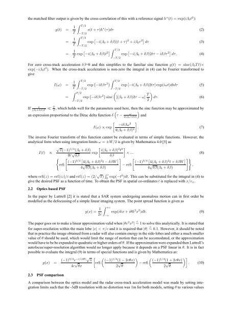
the matched filter output is given by the cross-correlation of this with a reference signal h ∗ (t) = exp(iβ 0 t 2 ):g(t) = 1 T= 1 T∫ T/2−T/2∫ T/2−T/2s(t + τ)h ∗ (τ)dτ (2)exp [ −i(β 0 + δβ)(t + τ) 2 + iβ 0 τ 2] dτ (3)= 1 T exp [ −i(β 0 + δβ)t 2] ∫ T/2exp [ −i(β 0 + δβ)2tτ − iδβτ 2] dτ. (4)−T/2For zero cross-track acceleration δβ=0 and this simplifies to the familiar sinc function g(t) = sinc(β 0 T t)×exp(−iβ 0 t 2 ). When the cross-track acceleration is non-zero the integral in (4) can be Fourier transformed togiveIfπ(β 0+δβ)T ≪ T 2I(ω) = 1 T=∫ T/2−T/2∫ T/2−T/2exp ( −iδβτ 2) ∫ T/2exp [−i(β 0 + δβ)2tτ] exp(iωt)dtdτ (5)exp ( −iδβτ 2) sincan expression proportional to the Dirac delta function δ−T/2([(β 0 + δβ)2τ − ω] T 2)dτ. (6), which holds well for the parameters used here, then the sinc function may be approximated by()τ − andω2(β 0+δβ)[ ] −iδβω2I(ω) ∝ exp4(β 0 + δβ) 2 . (7)The inverse Fourier transform of this function cannot be evaluated in terms of simple functions. However, theanalytical form when using integration limits ω = ±W/2 is given by Mathematica 4.0 [5] as√ π(−1) 1/4 [(β 0 + δβ)I(t) ∝W √ i(β0 + δβ) 2 t 2 ]exp× ... (8)δβδβ{ [ [ (−1)3/44(β 0 + δβ) 2 t − δβW ] ] [ [ (−1)3/44(β 0 + δβ) 2 t + δβW ] ]}erfi4 √ δβ(β 0 + δβ)− erfi4 √ δβ(β 0 + δβ)where erfi(z) = erf(iz)/i and erf(z) = (2/ √ π) ∫ z0 exp(−t2 )dt. This can be substituted for the integral in (4) togive the desired PSF as a function of time. To obtain the PSF in spatial co-ordinates t is replaced with x/v x .2.2 Optics based PSFIn the paper by Luttrell [2] it is stated that a SAR system undergoing anomalous motion can in first order bemodelled as the defocussing of a simple linear imaging system. The point spread function is given asg(x) = 1 2c∫ +c−cexp(ikx + iθk 2 x 2 )dk. (9)The paper goes on to make a linear approximation valid when |θc 2 x 2 | ∼ < 1 to solve this analytically. It is stated thatfor super-resolution within the main lobe |x| < π/c and it is required that |θ| ∼ < 0.1. However, it should be notedthat in practice the image obtained from a radar will also contain energy in the side-lobes and either a much smallervalue of θ should be used, which would limit the range of motion that can be accomodated, or the approximationwould have to be be expanded to quadratic or higher orders of θ. If the approximation were expanded then Luttrell’sautofocus/super-resolution algorithm would no longer apply because it depends on a PSF linear in θ. It is in factpossible to evaluate the integral (9) in terms of special functions and is given by Mathematica as:g(x) = (−1)3/4 e −i/(4θ)√ π4c √ θx2.3 PSF comparison[erfi( (−1) 1/4 (1 − 2cθx)2 √ θ)− erfi( (−1) 1/4 (1 + 2cθx)2 √ θ,)]. (10)A comparison between the optics model and the radar cross-track acceleration model was made by setting integrationlimits such that the -3dB resolution with no distortion was 1m for both models, setting θ to various values