Triola's The Basic Practice of Statistics Formulas & Tables

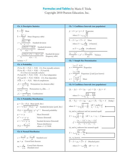
Formulas and Tables by Mario F. TriolaCopyright 2010 Pearson Education, Inc.Ch. 8: Test Statistics (one population)z = pN - pProportion—one populationn©xy - 1©x21©y2pqCorrelation r =2n1©x 2 2 - 1©x2 2 2n1©y 2 2 - 1©y2 2B nMean—one populationz = x - ms> 1n ( known)or r = a where zAz x z y Bx = z score for xz y = z score for yn - 1Mean—one populationt = x - mn©xy - 1©x21©y2( unknown)Slope:bs> 1n1 =n 1©x 2 2 - 1©x2 21n - Standard deviation or variance—x 2 12s2s= ys 2 one populationor b 1 = rs xCh. 9: Test Statistics (two populations)z = 1pN y-Intercept:1 - pN 2 2 - 1p 1 - p 2 2Two proportionspqB n+ pqb 0 = y - b 1 x or b 0 = 1©y21©x 2 2 - 1©x21©xy2n 1©x1 n 2 2 - 1©x2 22‹ p = x 1 + x 2n 1 + n 2t = 1x 1 - x 2 2 - 1m 1 - m 2 2yN = b 0 + b 1 x Estimated eq. of regression linedf smaller ofs 2 1n 1 1, n 2 1+ s2 2explained variationBn 1 nr 2 =2total variation‹ ‹F = s2 1s 2 2Two means—independent; s 1and s 2unknown, and notassumed equal.t = 1x 1 - x 2 2 - 1m 1 - m 2 2+ s2 pBn sp 2 = 1n 1 - 12s 2 1 + 1n 2 - 12s 2 21 n 2n 1 + n 2 - 2Two means—independent; s 1and s 2unknown, butassumed equal.Two means—independent;z = 1x 1 - x 2 2 - 1m 1 - m 2 2 1, 2known.s12B n+ s 221 n 2t = d - m ds d > 1ns 2 pStandard deviation or variance—two populations (where s 2 1 s 2 2 )Ch. 11: Goodness-of-Fit and Contingency Tables1O -x 2 E22= gE1O - Contingency tablex 2 E22= g [df (r 1)(c 1)]E1row total21column total2where E =1grand total21ƒb - c ƒ -x 2 122=b + c‹Two means—matched pairs(df n 1)Goodness-of-fit(df k 1)(df n 1 n 2 2)McNemar’s test for matchedpairs (df 1)Ch. 10: Linear Correlation/Regressions e = B©1y - yN2 2n - 2yN - E 6 y 6 yN + Eor B©y 2 - b 0 ©y - b 1 ©xyn - 2Prediction intervalwhere E = t a>2 s e 1 + 1 B n + n1x 0 - x2 2n1©x 2 2 - 1©x2 2Ch. 12: One-Way Analysis of VarianceProcedure for testing H 0 : m 1 = m 2 = m 3 = Á1. Use software or calculator to obtain results.2. Identify the P-value.3. Form conclusion:If P-value a, reject the null hypothesisof equal means.If P-value a, fail to reject the null hypothesisof equal means.Ch. 12: Two-Way Analysis of VarianceProcedure:1. Use software or a calculator to obtain results.2. Test H 0: There is no interaction between the row factor andcolumn factor.3. Stop if H 0from Step 2 is rejected.If H 0from Step 2 is not rejected (so there does not appear tobe an interaction effect), proceed with these two tests:Test for effects from the row factor.Test for effects from the column factor.

Formulas and Tables by Mario F. TriolaCopyright 2010 Pearson Education, Inc.Ch. 13: Nonparametric Tests1x + 0.52 - 1n>22z =1n>2z =z = R - m Rs R=H =BT - n 1n + 12>4n 1n + 1212n + 12Sign test for n 2512N1N + 12 a R 2 1+ R 2 2+ . . . + R 2 kb - 31N + 12n 1 n 2 n kKruskal-Wallis (chi-square df k 1)6©d 2r s = 1 -n1n 2 - 12acritical value for n 7 30:z = G - m Gs G=24Ch. 14: Control ChartsR - n 11n 1 + n 2 + 122BR chart: Plot sample rangesUCL: D 4 RCenterline: RLCL: D 3 Rx chart: Plot sample meansUCL: xx + A 2 RCenterline: xxLCL: xx - A 2 Rn 1 n 2 1n 1 + n 2 + 1212Rank correlationp chart: Plot sample proportionspqUCL: p + 3 B nCenterline: ppqLCL: p - 3 B nWilcoxon signed ranks(matched pairs and n 30); z1n - 1 bG - a 2n 1n 2n 1 + n 2+ 1b12n 1 n 2 212n 1 n 2 - n 1 - n 2 2B 1n 1 + n 2 2 2 1n 1 + n 2 - 12Wilcoxon rank-sum(two independentsamples)Runs testfor n 20TABLE A-6Critical Values of thePearson CorrelationCoefficient rn a = .05 a = .014 .950 .9905 .878 .9596 .811 .9177 .754 .8758 .707 .8349 .666 .79810 .632 .76511 .602 .73512 .576 .70813 .553 .68414 .532 .66115 .514 .64116 .497 .62317 .482 .60618 .468 .59019 .456 .57520 .444 .56125 .396 .50530 .361 .46335 .335 .43040 .312 .40245 .294 .37850 .279 .36160 .254 .33070 .236 .30580 .220 .28690 .207 .269100 .196 .256NOTE: To test H 0 : r = 0 against H 1 : r Z 0,reject H 0 if the absolute value of r isgreater than the critical value in the table.Control Chart ConstantsSubgroup Sizen A 2D 3D 42 1.880 0.000 3.2673 1.023 0.000 2.5744 0.729 0.000 2.2825 0.577 0.000 2.1146 0.483 0.000 2.0047 0.419 0.076 1.924

General considerations• Context of the data• Source of the data• Sampling method• Measures of center• Measures of variation• Nature of distribution• Outliers• Changes over time• Conclusions• Practical implicationsFINDING P-VALUESHYPOTHESIS TEST: WORDINGOF FINAL CONCLUSIONInferences about M: choosing between t and normal distributionst distribution:s not known and normally distributed populationor s not known and n 30Normal distribution: s known and normally distributed populationor s known and n 30Nonparametric method or bootstrapping: Population not normally distributed and n 30

NEGATIVE z Scoresz0TABLE A-2Standard Normal (z) Distribution: Cumulative Area from the LEFTz .00 .01 .02 .03 .04 .05 .06 .07 .08 .09-3.50andlower .0001-3.4 .0003 .0003 .0003 .0003 .0003 .0003 .0003 .0003 .0003 .0002-3.3 .0005 .0005 .0005 .0004 .0004 .0004 .0004 .0004 .0004 .0003-3.2 .0007 .0007 .0006 .0006 .0006 .0006 .0006 .0005 .0005 .0005-3.1 .0010 .0009 .0009 .0009 .0008 .0008 .0008 .0008 .0007 .0007-3.0 .0013 .0013 .0013 .0012 .0012 .0011 .0011 .0011 .0010 .0010-2.9 .0019 .0018 .0018 .0017 .0016 .0016 .0015 .0015 .0014 .0014-2.8 .0026 .0025 .0024 .0023 .0023 .0022 .0021 .0021 .0020 .0019-2.7 .0035 .0034 .0033 .0032 .0031 .0030 .0029 .0028 .0027 .0026-2.6 .0047 .0045 .0044 .0043 .0041 .0040 .0039 .0038 .0037 .0036-2.5 .0062 .0060 .0059 .0057 .0055 .0054 .0052 .0051 * .0049 .0048-2.4 .0082 .0080 .0078 .0075 .0073 .0071 .0069 .0068 .0066 .0064-2.3 .0107 .0104 .0102 .0099 .0096 .0094 .0091 .0089 .0087 .0084-2.2 .0139 .0136 .0132 .0129 .0125 .0122 .0119 .0116 .0113 .0110-2.1 .0179 .0174 .0170 .0166 .0162 .0158 .0154 .0150 .0146 .0143-2.0 .0228 .0222 .0217 .0212 .0207 .0202 .0197 .0192 .0188 .0183-1.9 .0287 .0281 .0274 .0268 .0262 .0256 .0250 .0244 .0239 .0233-1.8 .0359 .0351 .0344 .0336 .0329 .0322 .0314 .0307 .0301 .0294-1.7 .0446 .0436 .0427 .0418 .0409 .0401 .0392 .0384 .0375 .0367-1.6 .0548 .0537 .0526 .0516 .0505 * .0495 .0485 .0475 .0465 .0455-1.5 .0668 .0655 .0643 .0630 .0618 .0606 .0594 .0582 .0571 .0559-1.4 .0808 .0793 .0778 .0764 .0749 .0735 .0721 .0708 .0694 .0681-1.3 .0968 .0951 .0934 .0918 .0901 .0885 .0869 .0853 .0838 .0823-1.2 .1151 .1131 .1112 .1093 .1075 .1056 .1038 .1020 .1003 .0985-1.1 .1357 .1335 .1314 .1292 .1271 .1251 .1230 .1210 .1190 .1170-1.0 .1587 .1562 .1539 .1515 .1492 .1469 .1446 .1423 .1401 .1379-0.9 .1841 .1814 .1788 .1762 .1736 .1711 .1685 .1660 .1635 .1611-0.8 .2119 .2090 .2061 .2033 .2005 .1977 .1949 .1922 .1894 .1867-0.7 .2420 .2389 .2358 .2327 .2296 .2266 .2236 .2206 .2177 .2148-0.6 .2743 .2709 .2676 .2643 .2611 .2578 .2546 .2514 .2483 .2451-0.5 .3085 .3050 .3015 .2981 .2946 .2912 .2877 .2843 .2810 .2776-0.4 .3446 .3409 .3372 .3336 .3300 .3264 .3228 .3192 .3156 .3121-0.3 .3821 .3783 .3745 .3707 .3669 .3632 .3594 .3557 .3520 .3483-0.2 .4207 .4168 .4129 .4090 .4052 .4013 .3974 .3936 .3897 .3859-0.1 .4602 .4562 .4522 .4483 .4443 .4404 .4364 .4325 .4286 .4247-0.0 .5000 .4960 .4920 .4880 .4840 .4801 .4761 .4721 .4681 .4641NOTE: For values of z below -3.49, use 0.0001 for the area.*Use these common values that result from interpolation:z score Area-1.645 0.0500-2.575 0.0050

0 zPOSITIVE z ScoresTABLE A-2(continued ) Cumulative Area from the LEFTz .00 .01 .02 .03 .04 .05 .06 .07 .08 .090.0 .5000 .5040 .5080 .5120 .5160 .5199 .5239 .5279 .5319 .53590.1 .5398 .5438 .5478 .5517 .5557 .5596 .5636 .5675 .5714 .57530.2 .5793 .5832 .5871 .5910 .5948 .5987 .6026 .6064 .6103 .61410.3 .6179 .6217 .6255 .6293 .6331 .6368 .6406 .6443 .6480 .65170.4 .6554 .6591 .6628 .6664 .6700 .6736 .6772 .6808 .6844 .68790.5 .6915 .6950 .6985 .7019 .7054 .7088 .7123 .7157 .7190 .72240.6 .7257 .7291 .7324 .7357 .7389 .7422 .7454 .7486 .7517 .75490.7 .7580 .7611 .7642 .7673 .7704 .7734 .7764 .7794 .7823 .78520.8 .7881 .7910 .7939 .7967 .7995 .8023 .8051 .8078 .8106 .81330.9 .8159 .8186 .8212 .8238 .8264 .8289 .8315 .8340 .8365 .83891.0 .8413 .8438 .8461 .8485 .8508 .8531 .8554 .8577 .8599 .86211.1 .8643 .8665 .8686 .8708 .8729 .8749 .8770 .8790 .8810 .88301.2 .8849 .8869 .8888 .8907 .8925 .8944 .8962 .8980 .8997 .90151.3 .9032 .9049 .9066 .9082 .9099 .9115 .9131 .9147 .9162 .91771.4 .9192 .9207 .9222 .9236 .9251 .9265 .9279 .9292 .9306 .93191.5 .9332 .9345 .9357 .9370 .9382 .9394 .9406 .9418 .9429 .94411.6 .9452 .9463 .9474 .9484 .9495 * .9505 .9515 .9525 .9535 .95451.7 .9554 .9564 .9573 .9582 .9591 .9599 .9608 .9616 .9625 .96331.8 .9641 .9649 .9656 .9664 .9671 .9678 .9686 .9693 .9699 .97061.9 .9713 .9719 .9726 .9732 .9738 .9744 .9750 .9756 .9761 .97672.0 .9772 .9778 .9783 .9788 .9793 .9798 .9803 .9808 .9812 .98172.1 .9821 .9826 .9830 .9834 .9838 .9842 .9846 .9850 .9854 .98572.2 .9861 .9864 .9868 .9871 .9875 .9878 .9881 .9884 .9887 .98902.3 .9893 .9896 .9898 .9901 .9904 .9906 .9909 .9911 .9913 .99162.4 .9918 .9920 .9922 .9925 .9927 .9929 .9931 .9932 .9934 .99362.5 .9938 .9940 .9941 .9943 .9945 .9946 .9948 .9949 * .9951 .99522.6 .9953 .9955 .9956 .9957 .9959 .9960 .9961 .9962 .9963 .99642.7 .9965 .9966 .9967 .9968 .9969 .9970 .9971 .9972 .9973 .99742.8 .9974 .9975 .9976 .9977 .9977 .9978 .9979 .9979 .9980 .99812.9 .9981 .9982 .9982 .9983 .9984 .9984 .9985 .9985 .9986 .99863.0 .9987 .9987 .9987 .9988 .9988 .9989 .9989 .9989 .9990 .99903.1 .9990 .9991 .9991 .9991 .9992 .9992 .9992 .9992 .9993 .99933.2 .9993 .9993 .9994 .9994 .9994 .9994 .9994 .9995 .9995 .99953.3 .9995 .9995 .9995 .9996 .9996 .9996 .9996 .9996 .9996 .99973.4 .9997 .9997 .9997 .9997 .9997 .9997 .9997 .9997 .9997 .99983.50 .9999and upNOTE: For values of z above 3.49, use 0.9999 for the area.*Use these common values that result from interpolation:Common Critical ValuesConfidence Criticalz score AreaLevel Value1.645 0.95000.90 1.6452.575 0.99500.95 1.960.99 2.575

TABLE A-3t Distribution: Critical t ValuesArea in One Tail0.005 0.01 0.025 0.05 0.10Degrees ofArea in Two TailsFreedom 0.01 0.02 0.05 0.10 0.201 63.657 31.821 12.706 6.314 3.0782 9.925 6.965 4.303 2.920 1.8863 5.841 4.541 3.182 2.353 1.6384 4.604 3.747 2.776 2.132 1.5335 4.032 3.365 2.571 2.015 1.4766 3.707 3.143 2.447 1.943 1.4407 3.499 2.998 2.365 1.895 1.4158 3.355 2.896 2.306 1.860 1.3979 3.250 2.821 2.262 1.833 1.38310 3.169 2.764 2.228 1.812 1.37211 3.106 2.718 2.201 1.796 1.36312 3.055 2.681 2.179 1.782 1.35613 3.012 2.650 2.160 1.771 1.35014 2.977 2.624 2.145 1.761 1.34515 2.947 2.602 2.131 1.753 1.34116 2.921 2.583 2.120 1.746 1.33717 2.898 2.567 2.110 1.740 1.33318 2.878 2.552 2.101 1.734 1.33019 2.861 2.539 2.093 1.729 1.32820 2.845 2.528 2.086 1.725 1.32521 2.831 2.518 2.080 1.721 1.32322 2.819 2.508 2.074 1.717 1.32123 2.807 2.500 2.069 1.714 1.31924 2.797 2.492 2.064 1.711 1.31825 2.787 2.485 2.060 1.708 1.31626 2.779 2.479 2.056 1.706 1.31527 2.771 2.473 2.052 1.703 1.31428 2.763 2.467 2.048 1.701 1.31329 2.756 2.462 2.045 1.699 1.31130 2.750 2.457 2.042 1.697 1.31031 2.744 2.453 2.040 1.696 1.30932 2.738 2.449 2.037 1.694 1.30933 2.733 2.445 2.035 1.692 1.30834 2.728 2.441 2.032 1.691 1.30735 2.724 2.438 2.030 1.690 1.30636 2.719 2.434 2.028 1.688 1.30637 2.715 2.431 2.026 1.687 1.30538 2.712 2.429 2.024 1.686 1.30439 2.708 2.426 2.023 1.685 1.30440 2.704 2.423 2.021 1.684 1.30345 2.690 2.412 2.014 1.679 1.30150 2.678 2.403 2.009 1.676 1.29960 2.660 2.390 2.000 1.671 1.29670 2.648 2.381 1.994 1.667 1.29480 2.639 2.374 1.990 1.664 1.29290 2.632 2.368 1.987 1.662 1.291100 2.626 2.364 1.984 1.660 1.290200 2.601 2.345 1.972 1.653 1.286300 2.592 2.339 1.968 1.650 1.284400 2.588 2.336 1.966 1.649 1.284500 2.586 2.334 1.965 1.648 1.2831000 2.581 2.330 1.962 1.646 1.2822000 2.578 2.328 1.961 1.646 1.282Large 2.576 2.326 1.960 1.645 1.282

Formulas and Tables by Mario F. TriolaCopyright 2010 Pearson Education, Inc.x 2TABLE A-4 Chi-Square ( ) DistributionArea to the Right of the Critical ValueDegreesofFreedom 0.995 0.99 0.975 0.95 0.90 0.10 0.05 0.025 0.01 0.0051 — — 0.001 0.004 0.016 2.706 3.841 5.024 6.635 7.8792 0.010 0.020 0.051 0.103 0.211 4.605 5.991 7.378 9.210 10.5973 0.072 0.115 0.216 0.352 0.584 6.251 7.815 9.348 11.345 12.8384 0.207 0.297 0.484 0.711 1.064 7.779 9.488 11.143 13.277 14.8605 0.412 0.554 0.831 1.145 1.610 9.236 11.071 12.833 15.086 16.7506 0.676 0.872 1.237 1.635 2.204 10.645 12.592 14.449 16.812 18.5487 0.989 1.239 1.690 2.167 2.833 12.017 14.067 16.013 18.475 20.2788 1.344 1.646 2.180 2.733 3.490 13.362 15.507 17.535 20.090 21.9559 1.735 2.088 2.700 3.325 4.168 14.684 16.919 19.023 21.666 23.58910 2.156 2.558 3.247 3.940 4.865 15.987 18.307 20.483 23.209 25.18811 2.603 3.053 3.816 4.575 5.578 17.275 19.675 21.920 24.725 26.75712 3.074 3.571 4.404 5.226 6.304 18.549 21.026 23.337 26.217 28.29913 3.565 4.107 5.009 5.892 7.042 19.812 22.362 24.736 27.688 29.81914 4.075 4.660 5.629 6.571 7.790 21.064 23.685 26.119 29.141 31.31915 4.601 5.229 6.262 7.261 8.547 22.307 24.996 27.488 30.578 32.80116 5.142 5.812 6.908 7.962 9.312 23.542 26.296 28.845 32.000 34.26717 5.697 6.408 7.564 8.672 10.085 24.769 27.587 30.191 33.409 35.71818 6.265 7.015 8.231 9.390 10.865 25.989 28.869 31.526 34.805 37.15619 6.844 7.633 8.907 10.117 11.651 27.204 30.144 32.852 36.191 38.58220 7.434 8.260 9.591 10.851 12.443 28.412 31.410 34.170 37.566 39.99721 8.034 8.897 10.283 11.591 13.240 29.615 32.671 35.479 38.932 41.40122 8.643 9.542 10.982 12.338 14.042 30.813 33.924 36.781 40.289 42.79623 9.260 10.196 11.689 13.091 14.848 32.007 35.172 38.076 41.638 44.18124 9.886 10.856 12.401 13.848 15.659 33.196 36.415 39.364 42.980 45.55925 10.520 11.524 13.120 14.611 16.473 34.382 37.652 40.646 44.314 46.92826 11.160 12.198 13.844 15.379 17.292 35.563 38.885 41.923 45.642 48.29027 11.808 12.879 14.573 16.151 18.114 36.741 40.113 43.194 46.963 49.64528 12.461 13.565 15.308 16.928 18.939 37.916 41.337 44.461 48.278 50.99329 13.121 14.257 16.047 17.708 19.768 39.087 42.557 45.722 49.588 52.33630 13.787 14.954 16.791 18.493 20.599 40.256 43.773 46.979 50.892 53.67240 20.707 22.164 24.433 26.509 29.051 51.805 55.758 59.342 63.691 66.76650 27.991 29.707 32.357 34.764 37.689 63.167 67.505 71.420 76.154 79.49060 35.534 37.485 40.482 43.188 46.459 74.397 79.082 83.298 88.379 91.95270 43.275 45.442 48.758 51.739 55.329 85.527 90.531 95.023 100.425 104.21580 51.172 53.540 57.153 60.391 64.278 96.578 101.879 106.629 112.329 116.32190 59.196 61.754 65.647 69.126 73.291 107.565 113.145 118.136 124.116 128.299100 67.328 70.065 74.222 77.929 82.358 118.498 124.342 129.561 135.807 140.169From Donald B. Owen, Handbook of Statistical Tables, © 1962 Addison-Wesley Publishing Co., Reading, MA. Reprintedwith permission of the publisher.Degrees of Freedomn - 1 for confidence intervals or hypothesis tests with a standard deviation or variancek - 1 for goodness-of-fit with k categories(r - 1)(c - 1) for contingency tables with r rows and c columnsk - 1 for Kruskal-Wallis test with k samples