Download as a PDF - CiteSeer

The Long and Short of the Canada-U.S. Free Trade Agreement
∗ †
Daniel Treßer
University of Toronto
Canadian Institute for Advanced Research (CIAR)
and
National Bureau of Economic Research (NBER)
First Draft: June 1, 1998
This Revision: April 16, 2001
∗ Address: Institute for Policy Analysis, University of Toronto, 140 St. George Street, Suite 707, Toronto,
ON M5S 3G6. Telephone: (416) 978-1840. Facsimile: (416) 978-5519. E-mail: treßer@chass.utoronto.ca .
† IhavebeneÞted from the research assistance of Yijun Jiang, Huiwen Lai, and Susan Zhu. Conversations
on total factor productivity with Mel Fuss and Frank Lee have been central. Members of Statistics Canada
provided enormous help. These include Richard Barnabé (Standards Division), Jocelyne Elibani (International
Trade Division), Richard Landry (Investment and Capital Stock Division), Jean-Pierre Maynard
(Productivity Division), Bruno Pepin (Industry Division), and Bob Traversy (Industry Division). Gerry
Helleiner provided a healthy dose of scepticism. Michael Baker, Erwin Diewert, Peter Dungan, Aloysius
Siow and members of the CIAR provided key comments that dramatically improved the paper. Research
support from SSHRC is gratefully acknowledged.

Abstract
The Canada-U.S. Free Trade Agreement (FTA) provides a unique window on the effects
of trade liberalization. It was an unusually clean trade policy exercise in that it was not
bundled into a larger package of macroeconomic or market reforms. This paper uses the
1989-96 Canadian FTA experience to examine the short-run adjustment costs and long-run
efficiency gains that ßow from trade liberalization.
For industries subject to large tariff cuts (these are typically ‘low-end’ manufacturing
industries), the short-run costs included a 15% decline in employment and about a 10%
decline in both output and the number of plants. Balanced against these large short-run
adjustment costs were long-run labour productivity gains of 17% or a spectacular 1.0% per
year.
Although good capital stock and plant-level data are lacking, an attempt is made to
identify the sources of FTA-induced labour productivity growth. Surprisingly, this growth
is not due to rising output per plant, increased investment, or market share shifts to highproductivity
plants. Instead, half of the 17% labour productivity growth appears due to
favourable plant turnover (entry and exit) and rising technical efficiency.

The central tenet of international economics is that free trade is welfare improving. We
express our conviction about free trade in our textbooks and we sell it to our politicians. “It
is through the gradually increasing exposure of Canadian producers to competitive world-
market forces that the Canadian economy, as a whole, has become more productive,” states
Canada’s implementing legislation for NAFTA (Government of Canada 1994, page 70). Yet
the fact of the matter is that we have one heck of a time communicating this to the larger
public, a public gripped by Free Trade Fatigue.
Why is the message of professional economists not more persuasive? I think that there
are two reasons. First, in examining trade liberalization we treat short-run transition costs
and long-run efficiency gains as entirely separate areas of inquiry. On the one hand are those
who study the long-run productivity beneÞts of free trade policies e.g., Levinsohn (1993),
Harrison (1994), Tybout and Westbrook (1995), Krishna and Mitra (1998), and Pavcnik
(2000). On the other hand are those who study the short-run impacts of freer trade on
employment, earnings, and inequality e.g., Gaston and Treßer (1994, 1995), Feenstra and
Hanson (1996a, 1997), Revenga (1997), and Hanson and Harrison (1999). 1 Only Currie and
Harrison’s (1997) study of Morocco examines both labour market outcomes and productiv-
ity. Wearethusthinonresearchthatintegrateslong-runbeneÞts and short-run costs of
liberalization into a single framework. Nowhere is this more apparent than for the Canadian
experience with the Canada-U.S. Free Trade Agreement (FTA) and its extension to Mexico.
The FTA triggered on-going and heated debates about freer trade. This heat was generated
1 These papers deal with the impact of free trade policies. There are other papers that examine the effect
of increased trade without asking why trade increased e.g., Freeman and Katz (1991), Abowd and Lemieux
(1991), Revenga (1992), Bernard and Jensen (1995, 1997), Feenstra and Hanson (1996b, 1999), and Borjas,
Freeman, and Katz (1997).

y the conßict between those who bore the short run adjustment costs (displaced workers
andstakeholdersofclosedplants)andthosewhogarneredthelong run efficiency gains
(consumers and stakeholders of efficient plants).
There is another reason why the free trade message is not more persuasive. While case-
study evidence abounds about efficiency gains from liberalization (e.g., Krueger 1997), solid
econometric evidence for industrialized countries remains scarce. When I teach my students
about the effects of free trade on productivity I turn to high-quality studies for Turkey
(Levinsohn 1993), Cote d’Ivoire (Harrison 1994), Mexico (Tybout and Westbrook 1995),
India (Krishna and Mitra 1998), and Chile (Pavcnik 2000) among others. Even though I
Þnd these studies to be compelling, I wonder whether they can be expected to persuade
policy makers in industrialized countries such as Canada or the United States. What is
needed is at least some research focussing on industrialized countries.
The Canada-U.S. Free Trade Agreement offers several advantages for assessing the short-
run costs and long-run beneÞts of trade liberalization in an industrialized country. First,
the FTA policy experiment is clearly deÞned. In developing countries, trade liberalization
is typically part of a larger package of market reforms, making it difficult to isolate the
role of trade policy. Further, the market reforms themselves are often initiated in response
to major macroeconomic disturbances. Macroeconomic shocks, market reforms, and trade
liberalization are confounded. Indeed, Helleiner (1994, page 28) uses this fact to argue that
“Empirical research on the relationship between total factor productivity (TFP) growth and
... the trade regime has been inconclusive.” His view is widely shared e.g., Harrison and
Hanson (1999) and Rodriguez and Rodrik (1999). In contrast, the FTA was not implemented
2

as part of a larger package of reforms or as a response to a macroeconomic crisis. Second,
as Harrison and Revenga (1995, page 1) note, “Trade policy is almost never measured using
the most obvious indicators — such as tariffs.” See also Tybout (2000). This study of the
FTA is particularly careful about constructing pure policy-mandated tariff measures.
Third and perhaps most important, this paper examines the impacts of the FTA on a
large number of performance indicators in the manufacturing sector. These include imports,
value added, output, number of plants, plant size, labour productivity, total factor produc-
tivity, employment, skill upgrading, wages, hours of work, earnings, and income inequality.
Since each of these outcomes is examined using a common econometric framework, I am
better able to assess whether all my empirical ducks have lined up in a way that is consistent
with trade theory. In particular, I am better able to assess whether the results on long-run
beneÞts and short-run costs are consistent.
The FTA was implemented on January 1, 1989. I assess its impacts using ‘pre’ and
‘post’ Canadian data extending from 1980 to 1996. The data suffer two drawbacks. First,
capital stock is poorly measured which complicates productivity analysis. Second, plant-
level data are inaccessible so that I must work with manufacturing data at the industry
level. However, at some points of the paper I am able to exploit sub-industry level data on
plants grouped by plant size. These data form a balanced panel of 1,026 industry-plant size
observations in each year.
There is a body of econometric research on various aspects of the FTA (Beaulieu 2000,
Claussing 1995, Gaston and Treßer 1997, Government of Canada 1997, Head and Ries 1997,
1999a,b, Schwanen 1997, and U.S. Congress 1997). Each of these represents only one piece of
3

a larger puzzle whose picture depicts the many impacts of the FTA. For example, Claussing
(1995) focuses on trade effects, Gaston and Treßer (1997) only explore employment effects,
and Head and Ries (1999b) only examine plant size effects. Thus, none of the existing
studies can address the trade-offs between long-run efficiency gains and short-run adjustment
costs. In addition, this paper offers a large number of reÞnements that improve on existing
approaches.
This paper does not provide the silver bullet that makes the case either for or against
free trade. I offer clear evidence that the FTA created substantial long-run productivity
beneÞts. However, the short-run worker-displacement costs were also substantial. There
is thus a question of net beneÞts left hanging, but whose answer has been considerably
reÞned by the research to be presented. I hope that the results here take us one step closer
to understanding how freer trade can be implemented in an industrialized economy in a
way that recognizes both the long-run gains and the short-run adjustment costs borne by
workers and others.
1. The FTA Tariff Cuts: Too Small to Matter?
This paper deals with the impact of the FTA tariff cuts in manufacturing. It is therefore
natural to start by asking whether the FTA tariff cuts were deep enough to have mattered.
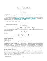
Recall that the FTA was implemented on January 1, 1989. The top panel of Þgure 1 plots
Canada’s average tariff rate against the United States in manufacturing. In 1988 it was 5.6
percent, a level too low to have had much effect. There are two problems with this claim.
First, tariffs tend to be lowest on less-processed manufactures and highest on processed ones.
4

Tariff Rates
Effective Tariff Rates
8%
6%
4%
2%
0%
20%
15%
10%
5%
0%
Figure 1. Canadian Tariff and Effective Tariff Rates
Canadian Tariff Rates Against:
Rest of the World
United States
80 81 82 83 84 85 86 87 88 89 90 91 92 93 94 95 96
Canadian Effective Tariff Rates Against:
Rest of the World
United States
80 81 82 83 84 85 86 87 88 89 90 91 92 93 94 95 96

For Canada this means that the tariff rate understates the effective rate of protection. The
bottom panel of Þgure 1 plots the effective rate of protection against the United States in
manufacturing. Effective rates of protection against the United States were twice as high
(11.3 percent in 1988) and have fallen more dramatically than nominal tariff rates. 2
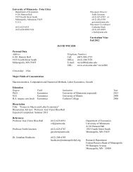
Second, low average tariffs disguise enormous differences in tariffs acrossindustries. Fig-
ure 2 plots a Lorenz curve for industry-level tariffs in 1988 and 1996. To derive this plot in
any year, say 1988, industries were sorted by their tariff rates. Let τ US
it be the Canadian tar-
iff against the United States in industry i in year t where i τ US
i+1,t. Let
nit be the percentage of Canadian 4-digit SIC industries with tariffs inexcessofτ US
it .There
are 213 industries so that, for example, an nit of 33 percent corresponds to 71 industries.
The Þgure plots τ US
it against nit. In 1988 almost 30 percent of all Canadian manufacturing
industries were sheltered behind a tariff in excess of 10 percent. By 1996 this number was
zero.
It is important to emphasize that Þgure 2 depends crucially on the level of aggregation.
If one moves from the plotted 4-digit data (213 industries) to 3-digit data (104 industries)
almost no industries had 1988 tariffs in excess of 10 percent. Thus the sample variation
associated with 4-digit disaggregation is a key feature of this study.
Another point to note is that the FTA called for reductions in U.S. tariffs against Canada.
I do not have U.S. tariff data at the level of disaggregation of interest. However, the
correlation between U.S. and Canadian bilateral tariffs in 1988 was very high (Magun et
2 Both the nominal and effective tariff rates were calculated at the 4-digit level as duties paid divided
by imports. They were aggregated up to all of manufacturing using 1980 Canadian production weights.
Appendix 1 provides details of my (standard) formula for the effective rate of protection.
5

Canadian Tariff Rates Against the U.S.
40%
35%
30%
25%
20%
15%
10%
5%
0%
Figure 2. Distribution of Tariffs Across Industries
1988
1996
0% 10% 20% 30% 40% 50% 60% 70% 80% 90% 100%
Percentiles of the Distribution of Canadian Manufacturing Industries
(n it )

al. 1988, Gaston and Treßer 1997, Head and Ries 1997). That is, Canada and the United
States were protecting the same industries. It is thus not surprising that with 2-digit SIC
data Gaston and Treßer (1997) found that once the Canadian tariff changes against the
United States are incorporated, it makes little difference if the U.S. tariffs against Canada
are added in. In addition, tariffs are positively correlated with effective tariffs and non-tariff
barriers to trade. In a regression setting this means that the tariff regressor will be picking
up the effects of U.S. tariffs, effective tariffs, and non-tariff barriers. This is precisely what
I want: When I analyze tariff reductions I am actually capturing a wider set of liberalizing
FTA policies.
2. The Data
In outlining a comprehensive assessment of the FTA the chief obstacle has been data prepa-
ration. Without high quality data all conclusions must be tentative. The database spans the
years 1980-96 and is at the 4-digit SIC level (213 manufacturing industries). The database
includes the most up to date information available and is unique in combining data from a
large number of disparate sources. All Canadian data are from Statistics Canada without
whose collective expertise nothing would have been possible. The variables may be divided
up into the following groups. (i) Imports, exports, and tariff duties from special tabula-
tions of the International Trade Division. (ii) Gross output, value added, number of plants,
employment, annual earnings, wages, and hours from special tabulations by the Canadian
Annual Survey of Manufactures (ASM) Section. (iii) The above ASM data by plant size,
again by special tabulation. (iv) Output and value-added deßators from the Input-Output
6

Division and the Prices Division. (v) Concordances from U.S. SIC (1987) and Canadian
SIC (1970) to Canadian SIC (1980) from the Standards Division.
Most of the U.S. data through 1994 are from the NBER Manufacturing Productivity
Database (Bartelsman and Gray 1996). The database was augmented and updated to 1996
using data from special tabulations done by the Bureau of Economic Analysis (BEA) and
from data available on the BEA and Bureau of Labor Statistics websites.
I will be working with industry-level data and industry-level data disaggregated by the
employment size of plants. I would have preferred using plant-level data. However, for legal
reasons these data have not yet been made publicly available. 3
3. Econometric Strategy
Let i index industries, let t index years, and let Yit be an outcome of interest such as
employment or productivity. The FTA was implemented on January 1, 1989. I have data
for the FTA period 1989-96 and the pre-FTA period 1980-88. For reasons to be explained,
it is useful to deÞne the FTA and pre-FTA periods without reference to data availability.
For choice of years t0 and t1with 1980

∆yis ≡
⎧
⎪⎨
⎪⎩
(ln Yi,t1 − ln Yi,1988)/(t1 − 1988) for s =1
(ln Yi,t0 − ln Yi,1980)/(t0 − 1980) for s =0
. (1)
∆yis approximates the annual compound growth rate of Yit during period s. Iaminterested
in a regression model explaining the impact of the FTA tariff cuts on industry outcomes of
interest:
where ∆τ FTA
is
∆yis = β∆τ FTA
is + γ∆xis + εis, s =0, 1 (2)
is a measure of the FTA mandated tariff concessions and ∆xis collects all
other determinants of ∆yis. The remainder of this section is devoted to a discussion of the
regression controls appropriate for equation (2).
3.1. The FTA Tariff Concessions
Interest in equation (2) focuses on the tariff term.Itistemptingtomeasure∆τ FTA
is
as the
change in Canadian tariffs against the United States during period s. However, as Þgure 1
above shows, tariffs were coming down against the rest of the world (i.e., against non-U.S.
trading partners) over this period. Thus, Canadian tariffs against the United States have a
strong trend that coincides with larger globalization trends. They thus potentially pick up
much more than just the FTA. Further, even in the absence of the FTA, tariffs wouldhave
come down as a result of the Uruguay Round. One can see this in Þgure 1 as the sharp drop
in Canadian tariffs against the rest of the world beginning in 1994. Let τ US
it be the Canadian
tariff against the United States in industry i in year t and let τ ROW
it
8
be the Canadian tariff

against the rest of the world. Then τ US
it − τ ROW
it
is the FTA mandated preferential tariff
concession extended to the United States. Its average annual change during the FTA period
(s =1)is
∆τ FTA
i1
³
≡ (τ US ROW
− τ ) − (τ i,t1 i,t1 US ROW
i,1988 − τ i,1988 )´ / (t1 − 1988) . (3)
Appendix table A1 lists the industries with the largest | ∆τ FTA
i1
of Þgure 1, ∆τ FTA
i1
and year t1.
|. In terms of the top panel
measures how the distance between the two lines changed between 1988
For the pre-FTA period, one expects the two lines to coincide because tariff rates were
primarily extended on a Most Favoured Nation (MFN) basis prior to 1988. One does not
see this for two reasons. First, the 1965 Canada-U.S. Auto Pact was a major exception to
MFN. I therefore let ∆τ FTA
i0
=((τUS ROW
i,t0 − τ i,t0 ) − (τ US
i,1980 − τ ROW
i,1980))/ (t0 − 1980) when i is an
automotive industry. 4 Second, while the underlying tariff rates on about 15, 000 commodities
usually obey MFN, they have been highly aggregated using import and production weights.
Aggregation causes the two lines to diverge. This raises a set of issues addressed in appendix
2. Since I do not want the results to be driven by aggregation bias, I impose ∆τ FTA
i0
when i is not an automotive industry.
As a tariff measure, ∆τ FTA
is
=0
has two advantages. First, it captures the core textual aspect
of the FTA. Second, its trend component is weak, indeed zero in the pre-FTA period. Thus,
much of the tariff data variability comes from the FTA period cross section. Implicitly, I
4 All results are the same with ∆τ FTA
i0
excluded from the analysis.
=0for the automotive sector or with the automotive sector
9

am comparing the performance of industries that were subjected to large tariff cuts with
the performance of industries that received small or zero tariff cuts. 5
3.2. The Secular Growth Control
I return now to the choice of ∆xis in equation (2). For political economy reasons, one
expects declining industries to have high tariffs (e.g.,Treßer 1993) and hence deep FTA
tariff cuts. One must therefore be careful not to attribute the effects of secular industry
decline to the FTA tariff cuts. Columns 1 and 2 of table 1 offer evidence on this by reporting
the cross-industry correlation of FTA period growth ∆yi1 with tariff cuts ∆τ FTA
i1
and pre-
FTA growth ∆yi0. The correlations are all positive, indicating that sluggish FTA period
growthcoincidedbothwithsluggishpre-FTAgrowthandwithlargeFTAperiodtariff cuts.
To prevent secular growth trends from being imputed to the FTA tariff cuts, I introduce
agrowthÞxed effect αi into equation (2):
∆yis = αi + β∆τ FTA
is
+ γ∆x 0
is + εis, s =0, 1. (4)
where ∆x 0
is is all other controls except αi. Asaresult,∆τFTA i1 canonlypickupFTAimpacts
on growth that are departures from trend growth. I now turn to the choice of ∆x 0
is .
5 It would be nice to exploit more of the within-industry changes in tariffs overtime. Inapreviousdraft
this was done by looking at speciÞcations in which all changes where annual i.e., there were 16 observations
per industry, one for each of the years in 1980-96. This means that there were 16 tariff changes recorded
for each industry. These annual-change results were similar to what will be repeated below. I no longer
report the annual change results because it is impossible to combine the annual change estimator with
adequate controls for business ßuctuations. As will become clear, controlling for business ßuctuations is
more important than squeezing out extra time-series variation in the data.
10

3.3. The U.S. Control
The 1990’s was a period of accelerating changes in technology as well as other determinants
of supply and demand. Thus, the secular growth captured by αi is not always a reliable
predictor of current growth. Further, these 1990’s changes were probably not conÞned to
Canada - they likely affected the United States as well. I thus control for underlying supply
and demand changes by introducing a U.S. control ∆yUS is into regression equation (4). ∆yUS is
is the U.S. counterpart to ∆yis. For example, if ∆yis is Canadian employment growth, ∆y US
is
is U.S. employment growth. Column (3) of table 1 reports the correlation of FTA period
Canadian growth ∆yi1 with U.S. growth ∆y US
i1 . The correlations are large and positive
which indicates that FTA period innovations in Canada and the United States shared a
common component. 6
It is tempting to argue that ∆y US
is is endogenous. That is, when Canadian industries do
well it is at the expense of their U.S. counterparts. If true, we should see it in one of two
ways. First, Canadian and U.S. growth should be negatively correlated. Yet I just showed
in column (3) of table 1 that these bivariate correlations are positive. Further, Gaston and
Treßer (1997) found positive multivariate correlations. (They looked at employment growth
using 2-digit data for the period 1980-93.) Thus, endogeneity is not evident in bivariate
6 The U.S. database is at the 4-digit level of 450 U.S. SIC industries whereas the Canadian data are at the
level of 213 Canadian SIC industries. I have converted the U.S. data into Canadian SIC using a Statistics
Canada electronic concordance called COMIND92 which is related to Statistics Canada’s catalogue 12-574
publication. Because some U.S. SIC industries do not go uniquely into a single Canadian SIC industry,
I have had to augment the Statistics Canada converter with more detailed U.S. data. Where there is no
uniqueness, U.S. industries were allocated to Canadian industries based on 5-digit U.S. value of shipment
weights. (The Þrst 4 digits are SIC industries, the last digit is a product code.) The weights used for year t
were year t data on either shipments, value added, or employment depending on the series being converted.
Data on 5-digit shipments are from the BEA website. With these data I was able to build a converter
that ‘steps down’ from over 1000 U.S. industry/products to 213 Canadian industries. I am indebted to my
research assistant Susan Zhu for taking on this mind-numbing, lengthy task.
11

or multivariate correlations of ∆yi1 with ∆y US
i1 . Second, if ∆y US
is is endogenous because
it was effected by FTA tariff cuts then ∆y US
is must be correlated with ∆τ FTA
i1 . In fact,
the correlation is virtually zero for each of the table 1 variables. The explanation for the
zero correlations is simple: The U.S. market is so large that the effect of the FTA was
swamped by more fundamental movements in industry demand and supply. It is exactly
these movements that I wish to proxy with ∆y US
is . I therefore amend equation (4) as follows:
∆yis = αi + β∆τ FTA
is
+ γ∆y US
is + δ∆x 00
is + εis, s =0, 1. (5)
where ∆x 00
is is all other controls except αi and ∆y US
is . I now turn to the choice of δ∆x 00
is.
3.4. The Business Conditions Control
A key issue for examining the FTA is the treatment of the early 1990’s recession. Figure
3 plots gross domestic product (gdp) for Canadian manufacturing. The data are in logs
relative to a 1980 base i.e., ln(gdpt/gdp1980). The FTA period recession stands out. General
business conditions can be introduced into equation (5) by including a regressor ∆zs that
measures movements in gdp, the exchange rate, Canada-U.S. interest rate differentials, and
other macro variables. However, one needs to allow industries to vary in their sensitivity to
general business conditions. That is, equation (5) needs a term ∆zs whose coefficient δi is
industry subscripted. Otherwise, if tariff cuts are deepest for the most cyclically sensitive
industries (e.g., low-end manufacturing), then the estimate of the tariff effect will be biased
12

ln(gdp t /gdp 1980 )
0.50
0.40
0.30
0.20
0.10
0.00
-0.10
Figure 3. Real Canadian Manufacturing GDP
Pre-FTA Period FTA Period
80 81 82 83 84 85 86 87 88 89 90 91 92 93 94 95 96 97 98
Notes : Data are from the series 'gdp at factor cost, 1992 dollars' from Statistics Canada's CANSIM database.

upward. I therefore amend equation (5) as follows:
∆yis = αi + β∆τ FTA
is
+ γ∆yUS is + δi∆zs + εis, s =0, 1 (6)
where I have replaced δ∆x 00
is with δi∆zs. αi, ∆τ FTA
is , ∆yUS is ,andδi∆zsare my regression
controls.
Estimating both the δi and the αi is a difficult problem, not least because it involves
estimating these 2 × 213 parameters with only 2 × 213 observations. Fortunately, there is a
simpler approach based on matching the FTA and pre-FTA business cycles. From Þgure 3,
there are a number of similarities between the 1980-88 and 1988-98 periods. Each begins a
year before the peak, enters a deep recession in the third year, and ends with a prolonged
expansion. This is not to minimize differences in the depth of the recessions or the pace of
their recoveries, but to point out useful similarities. By experimenting with the choice of
pre-FTA and FTA periods (i.e., t0 and t1 in equation 1), it is possible to place industries
at about the same point on the business cycle in each of the two periods. In this way, the
pre-FTA period data on business cycle sensitivity can be used to control for FTA period
business cycle sensitivity.
My preferred choice of periods uses t0 = 1986 and t1 = 1996 so that FTA changes cover
1988-96 and pre-FTA changes cover 1980-86. Relative to 1980-86, the 1988-96 period is one
year ahead as judged by the number of years into the expansion and less than one year
behind as judged by gdp growth. Clearly, there is some question about how best to choose
the periods. Fortunately, the empirical results are not particularly sensitive to this choice,
13

a fact that will be shown at length below. I therefore postpone further discussion of timing.
By the way, it is no coincidence that there were sufficient data for lining up the pre-FTA
and FTA business ßuctuations. In a previous draft I only had data back to 1984 because
that was the year that Statistics Canada changed its industrial classiÞcation from SIC(1970)
to SIC(1980). Obtaining data back to 1980 in order to match business ßuctuations involved
custom runs by Statistics Canada as well as the construction of a concordance between
Canadian SIC (1970) and Canadian SIC (1980) which, remarkably, existed previously only
in limited form. 7
3.5. Estimation
Moving to the formal estimation framework, I will difference equation (6) across the two
periods and use the fact that industries are at the same point on the business cycle in each
period (δi∆z1 = δi∆z0). Then
(∆yi1 − ∆yi0) =β(∆τ FTA
i1
− ∆τ FTA
i0 )+γ(∆y US
i1 − ∆y US
i0 )+υi. (7)
Such differencing eliminates 2 × 213 parameters from equation (6). Not only do the δi fall
out, but so do the αi along lines related to the Heckman and Hotz (1989) random growth
estimator. Equation (7), with an intercept, is my primary regression speciÞcation:
(∆yi1 − ∆yi0) =θ + β(∆τ FTA
i1
FTA
− ∆τ i0 )+γ(∆y US
i1
− ∆yUS
i0 )+υi. (8)
7 I am indebted to Paul Beaudry, Janet Currie, Paul Romer, Alwyn Young and other CIAR workshop
participants for insisting that I control for business cycles. I am also indebted to Richard Barnabé, Director
General of the Standards Division at Statistics Canada, for helping me to construct an SIC(1970) to
SIC(1980) converter.
14

The intercept is derived by adding a period dummy θs to equation (6) and deÞning θ ≡
θ1 − θ0.
I will also consider a simpler regression that eliminates the equation (6) secular growth
and business condition controls (αi and δi∆zs):
∆yis = θ + β∆τ FTA
is
+ γ∆y US
is + εis, s =0, 1. (9)
This speciÞcation helps pinpoint the impact of these controls on the estimate of β. I em-
phasize that equation (9) is used only for regression diagnostic purposes.
3.6. Endogeneity of Tariffs
Tariff cuts are not exogenous. They depend on industry characteristics e.g., Brock and
Magee (1978) and Treßer (1993). In the change-in-changes equation (8) setting, it is not clear
why endogeneity should be an issue. 8 However, one can always work up some story about
endogeneity. As such, I also consider instrumental variables (IV) estimates. The instrument
set consists of 1988 values for hourly wages (capturing protection for low-wage industries
as in Corden’s 1974 conservative social welfare function), the proportion of non-production
workers (capturing protection for unskilled industries), the level of output (capturing pro-
tection for large industries as in Finger, Hall, and Nelson’s 1982 high track protection for
large industries), imports, and exports. I also include all the cross—products. Since all these
8 ∆τ FTA
i1
FTA − ∆τ
i0
approximately equals ∆τ FTA
i1
(see the discussion following equation 3), and ∆τ FTA
i1
is largely determined by the tariff level in 1988. This in turn depends on industry characteristics in 1988.
There are two types of such characteristics, those expressed as levels in 1988 such as average wages and those
expressed as changes leading up to 1988 such as output growth. It is not clear why such levels or changes
should be correlated with changes in changes i.e., with the dependent variable ∆yi1 − ∆yi0 in equation (8).
15

variables are in 1988 levels, the assumption that they are uncorrelated with the double-
differenced error term is comfortable. Finally, I include ∆y US
i1 − ∆y US
i0 since this already
appears as an exogenous variable. I do not include any Canadian growth characteristics
such as ∆yi0 or ∆yi1 − ∆yi0 since these are arguably endogenous.
I have mixed feelings about the IV estimates. On the one hand, a number of factors
argue for emphasizing them. (i) The IV results invariably imply larger FTA impacts than do
the ordinary least squares (OLS) results. They thus strengthen my conclusions. (ii) TheIV
estimates are robust in that they are insensitive to the choice of instruments i.e., to different
variables, to the omission of cross-products, and to the omission of ∆y US
i1
− ∆yUS i0 .(iii) The
Þrst-stage R 2 s are always close to 0.4 which is arguably not ‘too’ high. On the other hand,
there are factors that argue against emphasizing the IV results. First, IV methods require
strong assumptions about instrument validity. Second and more important, the Hausman
test (Wu’s T2 test) rejects endogeneity for 17 of the 22 variables to be considered. For these
reasons, I will present the IV results, but not have much to say about them.
4. Empirical Results: Employment
Unlike most assessments of the impact of trade liberalization, this paper examines impacts
on a large number of performance indicators. I begin with employment. The results appear
in table 2. Since tables of this form will appear repeatedly, I carefully review it. Consider
the top block of rows which deal with the employment of all workers. The ‘Regression
SpeciÞcation’ columns state whether equation (8) or equation (9) is being estimated and
how the pre-FTA and FTA period changes are deÞned. For example, the Þrst line presents
16

estimates of equation (8) with the pre-FTA period changes deÞned over 1980-86 and the
FTA period changes deÞned over 1988-96. This is my preferred speciÞcation.
ReturningtotheÞrst line, the coefficient on the FTA tariff concessions is b β =1.51 which
indicates that the FTA reduced employment. The coefficient on the U.S. control is bγ =0.20.
The intercept is not reported. There are 213 observations and the R 2 is a modest 0.071.
In the second line, the pre-FTA period changes are re-deÞned to cover 1980-88 and in the
third line the FTA period changes are re-deÞned to cover 1988-94. As is apparent, our
results are only modestly sensitive to the choice of periods and hence to the implicit choice
of business-cycle control.
The last line gives estimates of the regression diagnostic equation (9). In this line there
are 426 (=2×213) observations because I have stacked the 2 periods. When the secu-
lar growth and business conditions controls are omitted, the FTA effect is much larger
( b β =2.29). This shows that in the absence of proper controls, it is easy to overstate the em-
ployment effects of the FTA. It thus vindicates the lengthy theoretical discussion of controls
in section 3.
The fourth row gives the IV estimate b β =2.70. As will generally be the case in this
paper, it is larger in magnitude than the OLS estimate. The column “Wu’s T2” gives the
p-value for the Wu-Hausman exogeneity test. The value of 0.106 indicates that endogeneity
is just rejected at the 10 percent level. Given the low power of the test, I will use Wu’s
T2 < 0.01 as a criterion for rejecting exogeneity.
The data distinguish between workers employed in manufacturing activities and non-
manufacturing activities. I will refer to these as production and non-production workers
17

since the distinction broadly follows that used in the U.S. Annual Survey of Manufactures
(ASM). In 1988, production workers earned 30 percent less than non-production workers.
An internal Statistics Canada memo also veriÞes that non-production workers are more
educated than production workers. Table 2 reports results separately for production and
non-production workers. The results for production workers are very similar to those of all
workers. Thus, the results for total employment are driven by production workers. The
FTA appears to have had almost no impact on non-production workers ( b β = 0.48 and
t =0.55). However, exogeneity is rejected and the IV estimate indicates that the FTA
raised non-production worker employment.
A common measure of average industry skill is the ratio of non-production workers to
production workers. Hence the change in this ratio is often referred to as ‘skill upgrading.’
The OLS results indicate that the FTA did not signiÞcantly contribute to skill upgrading
( b β = −1.35 and t = −1.35). However, the IV results paint a picture of statistically signiÞcant
FTA induced skill upgrading. This is consistent with a Feenstra and Hanson (1996a) story
involving Canadian outsourcing to low-wage, less-unionized Southern U.S. states. This was
an issue raised during the FTA negotiations.
5. Economic Impacts
For industry i, b β∆τ FTA
i1
is the log-point change in an outcome of interest such as employment
that is explained by the FTA mandated tariff cuts. To calculate the log-point change for all
of manufacturing one must compute the weighted average of the b β∆τ FTA
i1
where the weights
depend on industry size. See appendix 5 for details. The change in employment for all of
18

manufacturing appears in table 2. Consider the last line in the block of rows dealing with the
employment of all workers: ‘Observed Change = (-16%, -25%), Due to FTA = (-5%, -15%).’
Observed Change is the log point change in employment during 1988-96. In what follows I
will interpret these log point changes as percentage changes. The Þrst number in parentheses
(-16 percent) is the manufacturing-wide percentage change in employment. Employment fell
by 16 percent. Due to FTA is the log point change in employment estimated to have been
caused by the FTA mandated tariff cuts. With b β =1.51, I estimate that the FTA tariff
cuts reduced employment by 5 percent. Re-stated, about one-third (= 5/16) of the 1988-96
manufacturing employment losses are due to the FTA.
Of course, some industries experienced particularly large tariff cuts. I ranked the 213
manufacturing industries in my sample by the size of the FTA mandated tariff cuts (i.e.,
by the ∆τ FTA
i1 ) and examined the one-third of industries that experienced the deepest tariff
cuts. This group has 71 (= 213/3) industries. For these industries the production-weighted
average tariff cut was 10 percent, the smallest tariff cut was 5 percent and the largest
tariff cut was 33 percent. I will refer to these industries as the most impacted industries.
The industries are listed in table A1. As is apparent from table A1, these are ‘low-end’
manufacturing industries. Log point changes for these industries appear as the second
number in the parentheses following Observed Change and Due to FTA. For these industries,
employment fell by 25 percent and I estimate that the FTA reduced employment by 15
percent. Re-stated, about two-thirds (= 15/25) of the employment losses in the most
impacted industries were due to the FTA. These numbers point to the very large transition
costs of moving out of low-end, heavily protected industries. They are the most obvious of
19

the short-run costs associated with trade liberalization.
6. Earnings
Most commentators expected Canadian wages to suffer from competition from less-unionized,
less educated workers in the Southern United States. I assess this using annual earnings data
from ASM payroll statistics. See table 3. For all workers, the Observed Change row pro-
vides some evidence of downward earnings pressure. Earnings growth in the most impacted
industries was a scant 2 percent over 8 years compared to 5 percent for all industries. This
makes it particularly surprising that when inferences are based on a model with adequate
controls (i.e., equation 8), the FTA tariff concessions appear to have raised earnings. From
table 3, the tariff coefficient estimate is b β = −0.50 with a t-statistic of −2.61. Forthemost
impacted industries this translates into a modest, but positive 5 percent rise in earnings
over 8 years.
Inspection of table 3 reveals that the FTA earnings gains were completely driven by
earnings for production workers rather than non-production workers. This implies that
the FTA led to declining inequality as measured by the ratio of non-production worker
earnings to production worker earnings. This is conÞrmed by the table 3 results for ‘Earnings
Inequality.’ However, the reduction in inequality is not statistically signiÞcant.
Finally, table 4 shows that all of the earnings effect for production workers is due to FTA
effects on wages, not hours.
20

7. Imports
Table 5 presents results for the impact of the FTA tariff concessions on imports. The import
regressions do no include U.S. controls because this would make no sense. More sensible
controls can be introduced by scaling. In particular, I consider Canadian imports from the
United States as a share of Canadian output. I also consider Canadian imports from the
United States as a share of total Canadian imports. This captures import substitution.
From table 5, the FTA tariff cuts are a statistically signiÞcant determinant of these
import shares. From the Observed Change row, the FTA tariff cuts explain most of the
huge change in import shares experienced by the most impacted industries. For example,
the ratio of imports to output rose by 72 percent for the most impacted industries, a number
which is very similar to the 67 percent due to the FTA. Needless to say, the FTA cannot
explain the import surge among industries such as autos that were not effected by the FTA.
That is, the Due to FTA numbers for aggregate manufacturing are small.
For intra-industry trade, the results suggest that if anything, the FTA reduced such trade.
This is indicative of modest comparative advantage specialization. It is consistent with the
fuller discussion of specialization in Head and Ries (1999a). Note that my conclusion is not
statistically signiÞcant.
8. Output, Value Added and Number of Plants
Table 6 reports results for real output. Output is the value of shipments adjusted for
changes in inventories, goods in process, and goods for resale. Data are from a special
21

Statistics Canada run. I will discuss deßation issues in the next section. For now I note that
there is little sensitivity to choice of deßators. With an eye to later results on productivity,
I also prefer to work with output generated by production activities since it excludes non-
production activities such as in-house marketing, book-keeping and other service activities
for which productivity concepts are less clear. This said, results for production activities
and all activities are invariably similar. From the Observed Change row of table 6, output
rose by 9 percent during 1988-96 for all of manufacturing while it fell by 10 percent for the
most impacted industries. This is potentially strong evidence about the harm caused by the
FTA. However once controls for secular trends, business conditions, and U.S. movements
are added, this relationship is weakened (β =1.08 and t =1.76). The FTA reduced output
by a statistically insigniÞcant 11 percent for the most impacted industries.
Table 6 also reports results for real value added in production activities. Again, deßation
is discussed below. The most impacted industries experienced a 5 percent reduction in value
addedcomparedtoa6percentexpansioninvalueaddedforallofmanufacturing. However,
this relationship is neither statistically signiÞcant (t =0.37) nor economically large in the
multivariate regression setting of equation (8).
Over the 1988-96 period, the number of plants declined by 12 percent for all of manufac-
turing and by a staggering 23 percent for the most impacted industries. (See the Observed
Change row.) Once controls are added, the FTA effect becomes statistically small (t =1.74),
but remains economically large. For the most impacted industries, the FTA reduced the
number of plants by 8 percent. Thus, there remains evidence that the FTA led to plant
rationalization by accelerating exit.
22

To conclude, although the most impacted industries experienced large declines in output,
value added, and number of plants, FTA culpability appears to be only partial.
9. Labour Productivity
Ideally, one wants to examine productivity using a total factor productivity (TFP) measure.
Unfortunately, the Canadian ASM does not record capital stock or investment information.
There is thus little alternative but to work with labour productivity. The most common
measure of labour productivity is real value added per worker. This is the third measure
reported in table 7. There are several defects with this measure, two of which are easily
addressed.
The Þrst deals with the measurement of labour input. In Canada, but not in the United
States, there has been a strong trend towards part-time employment. By not correcting
for Canadian hours, measure 3 has a downward trend. Since this trend will be spuriously
correlatedwiththedownwardtrendintariffs, the estimated effect of the FTA on produc-
tivity ( b β ) will be downward biased. The Canadian data allow for an hours correction.
Unlike the U.S. data, value added is reported for production activities alone and thus can
be directly compared with the data reported for hours worked. Measure 1 of table 7 reports
bβ using Canadian real value added in production activities per hour worked and U.S. real
value added in all activities per employee. As expected, b β is larger for measure 3 than for
measure 1 (though both are large). Clearly, measure 1 is preferred.
The second data issue deals with deßators. 9 In table 7, measures 1 and 3 use output
9 I am indebted to Alwyn Young for encouraging me to examine this issue carefully.
23

deßators while measure 2 uses value-added deßators. Value-added deßators would have been
preferable had the U.S. deßator not been seriously ßawed for present purposes. It is at the
2-digit level (20 industries) and even at this highly aggregated level there are imputations
for instruments (SIC 38) and electric and electronic equipment (SIC 36). Measure 2 of table
7, the value-added deßated measure, thus has serious problems. This said, the b β based on
value-added deßators are very similar to the b β based on output deßators. This can be seen
by comparing measures 1 and 2 in table 7. 10
I now turn to a detailed review of the labour productivity results. Independent of
the measure of labour productivity, FTA tariff concessions raised labour productivity both
statistically and economically. For my preferred speciÞcation (the Þrst line of table 7),
theestimateoftheFTAtariff effect is b β = −1.56 with a t-statistic of −3.17. From the
Due to FTA row, this implies that the FTA raised labour productivity by 4.7 percent for
manufacturing as a whole and by 16.6 percent for the most impacted industries.
More generally, consider all the equation (8) OLS speciÞcations in table 7 that I have
reviewed so far i.e., the Þrst 3 lines for each measure. The b β range from -0.88 to -1.59 which
implies FTA induced productivity effects of 2.6 to 4.8 percent for manufacturing as a whole
and 9.3 to 16.9 percent for the most impacted industries. Thus, no matter which estimate
is used, large productivity gains obtain.
These numbers leave a greater impression when put on a compound annual basis. For
all of manufacturing, the FTA tariff concessions raised labour productivity by between 0.3
and 0.6 percent per year. For the most impacted industries, the tariff concessions raised
10 There are other problems with the deßators used in this study, but as an empirical matter these turn
out to be minor. I thus relegate them to appendix 4.
24

labour productivity by between 1.2 and 2.1 percent per year. Further, my preferred measure
1 puts the gains at the upper end of these intervals. These are enormous numbers. The idea
that an international trade policy could raise productivity so dramatically is to my mind
remarkable.
9.1. Some Additional Sensitivity
To further investigate robustness, I considered several additional speciÞcations for the mea-
sure 1 of labour productivity. These appear as the new block of 4 lines under measure 1.
(Similar conclusions emerge for the other measures.) In the Þrst of these lines ( b β = −1.52),
I exclude ∆y US
i1 as a regressor on the grounds that U.S. productivity growth in the high-tech
sector might be an inappropriate control for Canada. In the next line ( b β = −1.56), the 9
industries (observations) that comprise the automotive sector are deleted on the grounds
that this sector is distorted by the 1965 Auto Pact. In the next line ( b β = −1.38), I deleted
the 2 industries (observations) which, from table A1, might be viewed as having unusually
large FTA mandated tariff cuts. In the last line ( b β = −1.95), only those industries that
were among the 71 most impacted industries are included. (Here the sample size is down
to 71.) The similarity between the b β for the most impacted industries and for all of man-
ufacturing means that the estimates reported in table 7 adequately represent the former.
Lookingacrossthe4speciÞcations that I have reviewed in this subsection, it is clear that
the conclusions about large FTA induced increases in labour productivity are robust.
25

10. What Underlies Rising Labour Productivity?
Rising labour productivity could be driven by any number of factors. For example, capital
deepening and within-industry shifts to high productivity Þrms are obvious explanations.
In this section I take a systematic look at these and other explanations. I begin with a few
familiar equations. Let Q = A · F (L, K, M) be the production function for a representative
Þrm where Q is output, L is labour, K is capital, M is materials plus fuel, and A is a measure
of technical efficiency. Let αi (i = l, k, m) befactorshares.Forexample,αm = PmM/(PQ)
where P is the product price and Pm is the price of materials plus fuel. I allow for imperfect
competition with zero proÞts. Let µ be the elasticity of scale or, equivalently, the mark-up
of price over marginal cost. I will use lower case letters to denote log changes. For example,
a ≡ dA/A. Following Hall (1988), totally differentiate the log of the production function to
obtain
a is a common measure of productivity growth.
a = q − µ(αll + αkk + αmm). (10)
Now consider labour productivity growth. Value added is deÞned as V ≡ PQ− PmM.
Totally differentiating ln V − ln L, equating marginal revenue ∂PQ/∂Q with marginal cost
MC, and using MC = P (P/MC) −1 = Pµ −1 , one obtains an expression for labour produc-
tivity growth v − l:
v − l = q − µαmm − µ(1 − αm)l
. (11)
µ(1 − αm)
26

Consider the relationship between productivity growth a and labour productivity growth
v − l. In equation (10), substitute out αl using the zero-proÞt condition αl + αk + αm =1
and substitute out q − µαmm using equation (11) to obtain
a = µ {(1 − αm)(v − l) − αk(k − l)} . (12)
This equation provides a reference point for thinking about why labour productivity growth
v−l differs from productivity growth a. Interest focuses on the impact of trade liberalization
dτ on productivity i.e., on da/dτ. Fromequation(12),da/dτ depends on how µ, αm, (v −l),
αk, and(k − l) vary with dτ.
What follows is full of details so let me summarize it in advance. First, I will argue
empirically that d(k−l)/dτ and dµ/dτ are close enough to zero to be treated as second-order
effects. I will then compute da/dτ using data on the remaining terms. Empirically, the only
large term in the expression for da/dτ will be µ(1 − αm)d(v − l)/dτ. Sinceµ(1 − αm) ≈ 1/2
and d(v − l)/dτ is my estimate of the effect of the FTA on labour productivity, the effect of
the FTA on productivity is approximately half as large as its effect on labour productivity.
Finally, I will use data grouped by industry and plant size to argue that these productivity
effects are not due to shifts in market shares from low- to high-productivity plants. Rather,
they are due to plant turnover (entry and exit) together with rising technical efficiency.
10.1. Capital (d(k − l)/dτ)
4-digit capital stock does not exist for Canada. What is available is a wealth survey at
the 3-digit level for 1984-95. There are a number of problems with these data. First, at
27

the 3-digit level of 104 industries, much of the tariff variability disappears. Second, wealth
surveys are based on ownership rather than use so that most of the capital stock is assigned
to the Þnancial sector. (See Statistics Canada 1996). Third, the U.S. capital stock data
from the NBER productivity database are constructed very differently from the Canadian
data. With these caveats in mind, I proceed to estimation.
I estimate the usual equation (8) with ∆yis and ∆y US
is deÞned as changes in the log of the
Canadian and U.S. capital-labour ratios, respectively. The pre-FTA period changes cover
either 1984-86 or 1984-88 and the FTA period changes cover 1988-95. 11 Table 8 reports the
results. As is apparent, the FTA had no effect on the capital-labour ratio. To reÞne matters,
IalsodeÞned the Canadian capital-labour ratio on something closer to a production activity
basis: machinery and equipment divided by hours worked by production workers. Again,
there is no effectoftheFTAtariff cuts on the capital to labour ratio. Note that I am
precisely estimating zero effects. 12
None of this will surprise those involved in Canadian public policy where it is well known
that over the 1988-96 period, real Þxed investment grew by 74 percent in the U.S. compared
to only 15 percent in Canada. It is thus unlikely that the FTA labour productivity effect is
driven by capital deepening.
11 For this paper I updated the NBER productivity database from 1994 to 1996. However, I could not
update the capital stock data. Thus, for 1995 the U.S. capital stock data were extrapolated based on
1993-94 growth rates. This appears not to be important as judged by the fact that almost identical results
obtain when the FTA period changes cover 1988-94, thus excluding 1995.
12 SpeciÞcally, let bσ be the standard error of b β. If one replaces b β with b β ± bσ in the calculation of Due to
FTA, one still obtains effects that are less than 0.1 percent.
28

10.2. Scale (dµ/dτ)
From equation (12), the difference between productivity a and labour productivity v − l
depends on the scale of operations or mark-up µ. Work by Levinsohn (1993), Harrison
(1994), Krishna and Mitra (1998), and Pavcnik (2000) indicates that trade liberalization
has reduced mark-ups in developing countries. For the purpose of this section, which is
to investigate whether the FTA labour productivity results are driven by changes in µ, the
changes in µ documented by these authors are small. For example, one would need µ to
fall from 2.0 to 1.0 in order to argue that the FTA had no impact on productivity a. A
more realistic fall in µ, say from 1.1 to 1.0, would make little difference to my conclusions.
This point is explored in detail below.
Unfortunately, in the absence of good capital stock data, I cannot directly estimate either
µ or dµ/dτ. Nevertheless, there are some interesting insights to be garnered by examining
the effects of the FTA on proxies for µ. Very poor and dated proxies that hark back to
the pre-1980’s industrial organization literature are output per plant and value added per
plant. I estimate the usual equation (8) using these scale proxies. Note that I am back to
using 4-digit SIC data and that I do not have U.S. data for these scale proxies because U.S.
number-of-plants data are published only at 5-year intervals. The results appear in table 8.
As is apparent, the FTA impact on these proxies is statistically insigniÞcant and sensitive
to the choice of proxy.
I was initially surprised by the absence of FTA effects on output per plant. It contrasts
sharply with the computable general equilibrium literature. In many of those models it is
precisely scale effects that lead to much of the gains from trade. It is thus reassuring that
29

I arrive at the same conclusions as Head and Ries (1999b). It is all the more reassuring in
that I use a very different set of modelling assumptions. Tybout and Westbrook (1995) and
Tybout (2000) echo this theme of limited scale effects.
Mark-ups µ are the ratio of price to marginal cost. It is thus relevant to examine
prices. Returning to 3-digit data, the bottom of table 8 reports results for the impact of
the FTA on shipments deßators. The reduction in prices associated with the FTA tariff cuts
is statistically insigniÞcant and economically small.
To conclude, while I am conÞdent that the FTA had no impact on prices or output per
plant, I can only tentatively conclude from this that the FTA had no impact on scale or
mark-ups i.e., on µ.
10.3. Productivity (da/dτ)
The caveat-ridden conclusions of the last two subsections are that the FTA had little or no
effect on capital-labour ratios or scale economies. If so then a simple calculation relates FTA
induced productivity growth da/dτ to FTA induced labour productivity growth d(v −l)/dτ.
Differentiating equation (12) with respect to τ and using d(k − l)/dτ = dµ/dτ =0yields
da
dτ
= µ(1 − αm) d(v − l)
dτ
− µ
(
(v − l) dαm
dτ
+(k − l)dαk
dτ
)
. (13)
Table 9 calculates da/dτ for a particular set of assumptions about the terms in equation
(13). dτ is just a continuous version of the discrete change ∆τ FTA
i1 . d(v − l)/dτ is the
Due to FTA labour productivity effect from measure 1 of table 7. 13 v − l is the Observed
13 v is nominal value added growth. However, since we Þnd no evidence that the FTA effected value
30

Change data from measure 1 of table 7. k − l is the Observed Change data for machinery
and equipment per hour worked from table 8. For dαm/dτ and dαk/dτ, I use the observed
change in αm and αk during 1988-96 (times −1). This will overstate dαm/dτ and dαk/dτ,
but the associated terms are so small that any bias will have only second-order effects. For
the mark-up µ, Basu and Fernald (1997) and others argue that µ is small, close to unity
and no larger than 1.10. It makes no difference which µ²(1.00, 1.10) I use so that I settle
for µ =1.05. The reader can readily re-compute da/dτ for any value of µ by using equation
(13), table 9, and a hand-held calculator.
From table 9, the effect of the FTA on labour productivity is about twice as large as on a
i.e., on TFP. It raised TFP by 1.9 percent for all of manufacturing and by 7.7 percent for the
most impacted industries. On an annualized basis, the FTA raised TFP by a compounded
1.0 percent per year in the most impacted industries. To my mind, this number paints a
picture of very large long-run efficiency gains from trade liberalization.
Now that the reader has seen equation (13) and table 9, it is easy to show that it makes
little difference if the empirically motivated assumption dµ/dτ = 0 is relaxed. For the
most impacted industries (which are basically low-end manufacturing and hence subject to
constant returns to scale), a large change in µ would be 0.1 i.e., dµ/dτ = −0.1. Underthis
assumption, it is easy to show that the FTA effectforthemostimpactedindustriesfalls
from 7.7 percent to 6.7 percent. 14 That is, our estimate of the effect of the FTA tariff cuts
on TFP is not particularly sensitive to the assumption made about the effect of the FTA
added deßators, the change in nominal value added due to the FTA equals the change in real value added
due to the FTA.
14 From equation (12), ∂a/∂µ =(1 − αm)(v − l) − αk(k − l) ≈ 0.10 for the most impacted industries. If
dµ/dτ = −0.1 then ∂a/∂τ ≡ (∂a/∂µ)(dµ/dτ) ≈−0.010 or −1.0 percent.
31

tariff cuts on mark-ups.
Finally, one might ask if there is more direct evidence on TFP. The answer is yes. Using
some heroic assumptions about Canadian and U.S. data comparability, Statistics Canada
published 1990-95 TFP growth rates for 17 Canadian and U.S. industries. U.S. TFP growth
rates minus Canadian TFP growth rates appear in Þgure 4. I have ordered industries by the
depth of the FTA mandated tariff cuts: The most impacted industries are at the bottom and
the least impacted industries are at the top. Every one of the top 5 industries experienced
more rapid TFP growth in the United States than in Canada. Further, almost every one of
the bottom 5 industries experienced more rapid TFP growth in Canada than in the United
States. Figure 4 shows that Canadian TFP rose relative to U.S. TFP in those industries
that were most impacted by the FTA. This is exactly the same conclusion arrived at
econometrically in table 9.
10.4. Heterogeneity
It seems likely that part or most of the estimated FTA impact on productivity is not a gain
in technical efficiency, but industrial reallocation from low productivity to high productivity
plants. In this section I offer some informal evidence about the decomposition of FTA
labour productivity growth into its technical (within-plant) and allocative (between-plant)
components. I have 1988 and 1995 data on labour productivity grouped by industry and
plant size where plant size is deÞned by the number of employees e.g., all plants in SIC
industry 1011 with between 10 and 19 employees. The data are from special tabulations
by Statistics Canada and cover 204 of the 213 industries in my sample. There are 1,026
32

Figure 4. Annual TFP Growth Rate Differences, 1990-95
Industrial and Commercial Machinery
Printing and Publishing
Primary Metals
Food & Beverages
Electrical and Electronic Machinery
Petroleum Refining
Pulp and Paper
Transportation Equipment
Wood and Lumber
Fabricated Metal Products
Non-metallic Mineral Products
Chemical Products
Rubber and Plastic Products
Leather Products
Textiles
Furniture and Fixtures
Clothing
7.1%
-1.0% -0.5% 0.0% 0.5% 1.0% 1.5% 2.0% 2.5%
Difference Between U.S. and Canadian TFP Growth
Notes : The figure plots the annual percentage change in U.S. TFP less the annual percentage
change in Canadian TFP. Industries are sorted by the depth of the 1988-96 FTA-mandated
tariff cuts. Industries at the bottom of the figure experienced the deepest tariff cuts. For
Electrical and Electronic Machinery, the change of 7.1% is plotted as 2.2% in order to make
the figure clearer. Data are from Statistics Canada's The Daily , March 23, 1999.

industry-plant size cells and the median industry has 6 plant size groups. It is thus a rich
source of data. Let i continue to index industries and let j index plant size classes. Let yijt
be the log of some outcome of interest. The usual decomposition of total growth into its
within and between components is
X
i,j
yij,95ωij95 − X
yij,88ωij,88 =
i,j
X
(yij,95 − yij,88)ωij,88 +
i,j
X
(ωij,95 − ωij,88)yij,95
i,j
where ωijt is the usual cell weight for the industry-plant size cell (Σijωijt =1). 15 The three
terms in equation (14) are the ‘total,’ ‘within’ and ‘between’ changes, respectively. I will
denote them by ∆y T , ∆y W ,and∆y B , respectively.
Table 10 reports ∆y W , ∆y B , ∆y T and ∆y W /∆y T for variables of interest. The Þrst
observation is that 78 percent of labour productivity growth is within industry-plant size
cells. This is almost identical to the plant-level results reported by Baily et al. (1992) for
1982-87 U.S. TFP growth. Thus, most of FTA period labour productivity growth occurred
within industry-plant size cells. A secondary conclusion pointed to by the value added
and hours rows is that the productivity gains are coming from labour ‘shedding’: Within
industry-plant size cells, value added is not changing, but hours are falling.
It is still possible that the industries which experienced the deepest tariff cuts tended to
have share shifts favouring the most productive plants. To investigate the possibility of large
between-cell effects for the most impacted industries, I considered a variance decomposition
15 In the case of labour productivity, ωijt is (i, j)’s share of manufacturing value added. In the case of
output per plant, ωijt is (i, j)’s share of manufacturing output.
33
(14)

for each industry. That is, Þx industry i and compute
X
j
yij,95ω 0
ij95 − X
yij,88ω
j
0
ij,88 = X
(yij,95 − yij,88)ω
j
0
ij,88 + X
j
(ω 0
ij,95 − ω 0
ij,88)yij,95
where ω 0
ijt is the usual plant size weight for plant size j (Σjω 0
ijt =1). The three terms
in equation (15) will be denoted by ∆y T i , ∆y W i ,and∆y B i , respectively. The correlation
of ∆τ FTA
i1 with ∆y B i /∆y T i is a statistically insigniÞcant 0.04. That is, the most impacted
industries did not experience greater share shifting towards productive plants. Restated,
FTA induced labour productivity growth is unlikely to have been driven by shifts in market
share from low- to high-productivity plants.
There is another interesting result in table 10. For output per plant, growth between
industry-plant size cells accounts for 73 percent of total growth. This conÞrms what we
discussed before, namely, that any trend towards increased output per plant is associated
with a shift in market share to larger plants. By adding a plant size dimension, this result
extends the Head and Ries (1999b) observation that the FTA did not drive Þrms down
their average cost curves. It also extends the Tybout and Westbrook (1995) observations
for Mexico into a developed-country context.
Does the fact that most of the labour productivity growth was within industry-plant
size cells tell us that the observed labour productivity growth primarily reßects growth in
technical efficiency rather than growth in allocative efficiency? Not quite. I have ignored
entry and exit. While it is not aprioriclear whether plant turnover belongs in the ‘between’
34
(15)

or ‘within’ categories, Baldwin (1995) argues at length using 1970-79 Canadian plant data
that Canadian productivity growth due to plant turnover mostly occurred within industry-
plant size cells. Baldwin further Þnds that entering plants tended to be more productive
than exiting plants. Bernard and Jensen (1999) report a similar Þnding for the United
States. 16 Thus, labour productivity growth associated with entry and exit is likely part of
what is driving the observed labour productivity growth within industry-plant size cells.
This position is buttressed by the table 6 results which document that the FTA induced
large net exit.
Where is the rising technical efficiency coming from? Baldwin and Beckstead (2001)
argue that plants responded to the FTA tariff cuts by reducing the number of product lines.
Other sources of technical efficiency are also possible, including efficiency gains related to
the skill upgrading documented in table 2 above.
To conclude, FTA labour productivity growth does not appear to be caused by shifting
market share from low- to high-productivity plants. Rather, it appears to be explained both
by plant turnover (entry and exit) and rising technical efficiency within plants. 17
10.5. Productivity Conclusions
I examined the role of scale, capital deepening, materials usage, and plant heterogeneity
for my conclusions about labour productivity. If one is prepared to put aside the serious
problems caused by lack of good capital-stock data, then it appears that scale and capital
16 This may be related to Griliches and Regev’s (1995) ‘shadow of death.’ See Tybout (2000) for a review
of the literature that indicates how common is the Þnding that entering plants are more productive than
exiting plants.
17 We cannot be sure which is most important. Both Baily et al. (1992) and Griliches and Regev (1995)
Þnd that productivity gains are primarily due to within-plant gains rather than entry and exit.
35

deepening are not part of the FTA productivity story. If so, then half of the FTA impact
on labour productivity is attributable to an FTA impact on industry-level TFP. This latter
impact is large. Further, this change in industry-level TFP likely reßects a mix of plant
turnover and rising technical efficiency within plants.
While the absence of plant-level and capital stock data dampens my certainty about these
conclusions, the big picture is clearer. The most impacted industries are best characterized
as low-end manufacturing industries. See table A1. Thus, unless low-end manufacturing
experienced unusually high investment rates or enormous declines in mark-ups, the FTA
must have induced TFP growth. There is sufficient evidence at the 3-digit SIC level to be
conÞdent that low-end manufacturing did not experience an investment boom. Further,
the fact that low-end manufacturing typically has small mark-ups makes it impossible for
low-end manufacturing to have experienced enormous declines in mark-ups. Thus, it seems
likely that the FTA induced signiÞcant TFP growth through a combination of plant turnover
and rising technical efficiency within plants.
11. Conclusions
The FTA lives in two different worlds. For some, it is integral to employment losses and
eroding productivity relative to the United States. To others, it brought explosive trade
growth and large gains in manufacturing gdp. Both these views rest on aggregate numbers
for manufacturing. Neither is supported by a careful sectoral analysis. The following are
the main conclusions of sectoral analysis. I summarize these conclusions separately for
manufacturing as a whole and for the most impacted industries. The latter are the one-
36

third of industries which experienced the largest tariff cuts over the 1988-96 period. For
this group the tariff cuts ranged between 5 and 33 percent and averaged 10 percent.
(1) For the most impacted industries, the tariff cuts reduced employment by 15 percent,
reduced output by 11 percent, and reduced the number of plants by 8 percent. For man-
ufacturing as a whole, the numbers are 5, 3, and 4 percent, respectively. These numbers
capture the large adjustment costs associated with reallocating resources out of protected,
inefficient, low-end manufacturing. The fact that manufacturing employment and output
have largely rebounded since 1996 suggests that some and perhaps most of the reallocation
has been to high-end manufacturing.
(2) The tariff cuts raised labour productivity by a compounded annual rate of 2.1 percent
for the most impacted industries and by 0.6 percent for manufacturing as a whole. The tariff
cuts also raised total factor productivity by a compounded annual rate of 1.0 percent for
the most impacted industries and by 0.2 percent for manufacturing as a whole. We argued
that rising total factor productivity is not due to scale effects, capital deepening, or market
share shifts towards high productivity Þrms. Rather, it is due to a mix of plant turnover
and rising technical efficiency within plants. Dramatically higher productivity in low-end
manufactures and resource re-allocation to high-end manufactures are the key gains from
the FTA.
(3) Surprisingly, the tariff cuts slightly raised annual earnings, primarily by raising pro-
duction worker wages by 0.8 percent per year for the most impacted industries and by 0.3
percent per year for manufacturing as a whole. The tariff cuts did not effect earnings of
non-production workers or weekly hours of production workers. The FTA thus reduced
37

inequality, albeit minimally.
(4) For the most impacted industries, the tariff cuts explain almost all of the increased
trade with the United States and the increased U.S. share of Canadian trade.
Most of the effects of the FTA tariff cuts are smaller than one would imagine given the
heat generated by the debate. This heat is generated by the conßict between those who
bore the short run adjustment costs (displaced workers and stakeholders of closed plants)
and those who are garnering the long run productivity gains (consumers and stakeholders of
efficient plants). One cannot understand current debates about freer trade without under-
standing this conßict. The results here thus take us one step closer to understanding how
freer trade can be implemented in an industrialized economy in a way that recognizes both
the long-run gains and the short-run adjustment costs borne by workers and others.
38

Appendix
1. The Effective Rate of Protection: Let υj be value added in industry j per dollar
of output in the absence of tariffs. Let aij be the value of input of good i per dollar value of
the output of j in the absence of tariffs. Let τ j be the tariff rate against products in industry
j. Theeffective tariff τ e j is the amount by which the tariff structure (τ 1, ..., τ j,...,τ J) raises
value added in industry j. Following Basevi (1966),
τ e j = τ j +(τj − τ j) X
aijτ i/υj
i
where τ j = X
aijτ i/ X
For post-1992 effective rates of protection, the 1992 input-output table was used. In all
years, the effective rate of protection is calculated at the input-output ‘M’ level (which is
roughly at the 3-digit SIC level) and aggregated using production weights. The aggregated
data of Þgure 1 use 1980 production weights for aggregation and were smoothed using a
3-year moving average to eliminate a spike in 1993-94.
2. Tariff Aggregation Bias: Aggregation bias (the use of imports as weights for
aggregating tariffs to the 4-digit level) leads to violations of the Most-Favored Nation (MFN)
equality τ US
it = τ ROW
it for t ≤ 1988. Aggregation bias is only a problem in the present context
if it changes over time. Imposing τ US
i,1988 = τ ROW
i,1988 in equation (3) exacerbates such change
because it implicitly uses arbitrary aggregation weights for 1988 that are unrelated to the
import aggregation weights used for year t1. That is, it forces the aggregation weights to
change dramatically between 1988 and t1. This increases the change in aggregation bias
in the FTA period. As a result, I do not impose τ US
i,1988 = τ ROW
i,1988 in equation (3). To
39
i
i
aij.

investigate further, I also considered speciÞcations with ∆τ FTA
i0 =0replaced by ∆τ FTA
i0 ≡
((τ US ROW
i,t0 − τ i,t0 ) − (τ US
i,1980 − τ ROW
i,1980))/(t0 − 1980). This had little or no effect on the results.
3. List of Industries in Each Tariff Group: See table A1. Note that 12 of Canada’s
225 4-digit SIC industries were either excluded from the analysis because of incomplete data
or aggregated in order to ensure consistency over time. The aggregated industries are (new
name in parentheses): 1094 and 1099 (1098); 1511 and 1599 (1598); 1995 and 1999 (1998);
2911 and 2919 (2918); 2951 and 2959 (2958); 3051 and 3059 (3058); 3351 and 3359 (3358);
3362 and 3369 (3368).
4. Deßators:
U.S. Deflators: The value-added deßator is the gdp deßator reported on the BEA
website as of May 1999. The output deßator is the usual value of shipments deßator.
Through 1994, it is adjusted by Make tables as described in Bartelsman and Gray (1996).
After 1994, it is unadjusted. To see the effect of this series break, in table 7 compare the
Þrst and third lines for the output-deßated productivity measures. The Þrst line ends in
1996, the third in 1994. Since the estimates are similar, the splicing of the 1980-94 and
1995-96 deßator series plays little role. On a technical note, in converting deßators from
U.S. SIC to Canadian SIC, Tornqvist indexes were used.
Canadian Deflators: The value-added (output) deßator is derived by dividing nominal
value added (output) by real value added (output). The real and nominal series for value
added and output are from the Canadian input-output tables. The tables are available
through 1995. For 1996 both the value added and output deßators were spliced to the
Canadian ‘industry price indexes’ from CANSIM. This series is almost identical to the
40

input-output-derived output deßator, but not of course to the value added deßator. Again
from table 7, comparison of the Þrst line (ending in 1996) with the third line (ending in 1994)
reveals that the splice plays little role. The input-output tables are roughly at the 3-digit
Canadian SIC level (137 industries) so that the deßator values were repeated at the 4-digit
level (213 industries). It is difficult to evaluate the importance of this. Note though that
the simple correlation of tariff cuts ∆τ FTA
i1
with the output deßator is -0.04. This suggests
that cross-sectionally, the results are not being driven by a spurious correlation hidden here.
5. DeÞning ‘Observed Change’ and ‘Due to FTA’: Recall that Yi,1988 is the level
of, say employment, in industry i in 1988. The industry i change in employment over the
FTA period is approximately (∆yi1) Yi,1988 i.e., the log change times the initial level. The
change in employment among industries in any set I is approximately P
i²I (∆yi1) Yi,1988.
As a proportion of total employment it is P
i²I (∆yi1) Yi,1988/ P
j²I Yj,1988. This can be re-
written as P
i²I ∆yi1ωi where ωi ≡ Yi,1988/ P
j²I Yj,1988. 18 Using the fact that d ∆yi1 = b β∆τ FTA
i1
is the prediction of the impact of the tariff concessions, the predicted tariff-induced log
change in employment is P
i²I b β∆τ FTA
i1 ωi. Withthisinmind,Observed Change is deÞned
as 100 · 8 · P
∆yi1ωi and Due to FTA is deÞned as 100 · 8 · P bβ∆τ FTA
i1 ωi. Multiplying by 8
i²I
converts the average annual changes for the 8 FTA years into a total FTA period change.
For the compounded annual rates reported in this paper, the ‘8’ is removed. The b β used
in Due to FTA is the estimate from the Þrst-line speciÞcation (equation 8 with pre-FTA
period changes over 1980-86 and FTA period changes over 1988-96).
18 For the cases of production worker earnings and wages, ωi is based on total hours worked by production
workers. For the cases of skill upgrading and inequality ωi is based on total employment. For cases
where Yi,1988 is a ratio, ωi is based on the numerator of the ratio i.e., if Yi,1988 = ai,1988/bi,1988 then
ωi ≡ ai,1988/ P
j²I aj,1988.
41
i²I

References
Abowd, John M. and Lemieux, Thomas. “The Effects of Product Market Competition
on Collective Bargaining Agreements: The Case of Foreign Competition in
Canada,” in John M. Abowd and Richard B. Freeman, eds., Immigration, Trade, and
the Labor Market. Chicago: University of Chicago Press, 1991, pp. 343-67.
Baily, Martin Neil; Hulten, Charles and Campbell, David. “Productivity Dynamics
in Manufacturing Plants.” Brookings Papers: Microeconomics, 1992, pp. 187-249.
Baldwin, John R. The Dynamics of Industrial Competition: A North American Perspective.
Cambridge, MA: Cambridge University Press, 1995.
Baldwin, John R. and Beckstead, Desmond. “Changes in the DiversiÞcation of Canadian
Manufacturing Firms (1973-1997).” Mimeo, Statistics Canada, March, 2001.
Bartelsman, Eric J. and Gray, Wayne. “The NBER Manufacturing Productivity
Database.” National Bureau of Economic Research (Cambridge, MA) Technical Working
Paper No. 205, October 1996.
Basevi, Giorgio. “The United States Tariff Structure: Estimates of Effective Rates of
Protection of United States Industries and Industrial Labor.” Review of Economics
and Statistics, May 1966, 48(2), pp. 147-160.
Basu, Susanto and Fernald, John G. “Returns to Scale in U.S. Production: Estimates
and Implications.” Journal of Political Economy, April 1997, 105(2), pp. 249-83.
Beaulieu, Eugene. “The Canada-U.S. Free Trade Agreement and Labour Market Adjustment
in Canada.” Canadian Journal of Economics, May 2000, 33(2), pp. 540-63.
Borjas, George J.; Freeman, Richard B. and Katz, Lawrence F. “HowMuchDo
Immigration and Trade Affect Labor Market Outcomes?” Brookings Papers: Economic
Activity. 1997, (1), pp. 1-67.
Brock, William A. and Magee, Stephen P. “The Economics of Special Interest Politics:
The Case of the Tariff.” American Economic Review, May 1978 (Papers and
Proceedings), 68(2), pp. 246-50.
Bernard, Andrew B. and Jensen, J. Bradford. “Exporters, Jobs, and Wages in
U.S. Manufacturing: 1976-1987.” Brookings Papers on Economic Activity, 1995, pp.
67-112.
––––. “Exporters, Skill Upgrading, and the Wage Gap.” Journal of International
Economics, February 1997, 42(1-2), pp. 3-31.
––––. “Exporting and Productivity.” National Bureau of Economic Research (Cambridge,
MA) Working Paper No. 7135, May 1999.
42

Claussing, Kimberly A. “The Canada-U.S. Free Trade Agreement: Stepping Stone or
Stumbling Block.” Mimeo, 1995.
Corden, W. M. Trade Policy and Economic Welfare. Oxford: Clarendon Press, 1974.
Currie, Janet and Harrison, Ann E. “Sharing the Costs: The Impact of Trade Reform
on Capital and Labor in Morocco.” Journal of Labor Economics, July 1997, 15(3),
pp. S44-71.
Feenstra, Robert C. and Hanson, Gordon H. “Foreign Investment, Outsourcing, and
Relative Wages,” in R.C. Feenstra, G.M. Grossman and D.A. Irwin, eds., The Political
Economy of Trade Policy: Papers in Honor of Jagdish Bhagwati. Cambridge, MA:
MIT Press, 1996a, pp. 89-127.
––––. “Globalization, Outsourcing, and Wage Inequality.” American Economic Review,
May 1996b, 86(2), pp. 240-45.
––––. “Foreign Direct Investment and Relative Wages: Evidence from Mexico’s
Maquiladoras.” Journal of International Economics, May 1997, 42(3-4), pp. 371-93.
––––. “The Impact of Outsourcing and High-Technology Capital on Wages: Estimates
for the United States, 1979-1990.” Quarterly Journal of Economics, August 1999,
114(3), pp. 907-40.
Finger, J. Michael; Hall, H. Keith and Nelson, Douglas R. “The Political Economy
of Administered Protection.” American Economic Review, June 1982, 72(3), pp. 452-
66.
Freeman, Richard B. and Katz, Lawrence F. “Industrial Wage and Employment
DeterminationinanOpenEconomy,”inJohnM.AbowdandRichardB.Freeman,
eds., Immigration, Trade, and the Labor Market. Chicago: University of Chicago
Press, 1991, pp. 335-59.
Gaston, Noel and Treßer, Daniel. “Protection, Trade, and Wages: Evidence from
U.S. Manufacturing.” Industrial and Labour Relations Review, July 1994, 47(4), pp.
574-593.
––––. “Union Wage Sensitivity to Trade and Protection: Theory and Evidence.”
Journal of International Economics, August 1995, 39(1-2), pp. 1-25.
––––. “The Labour Market Consequences of the Canada-U.S. Free Trade Agreement.”
Canadian Journal of Economics, February 1997, 30(1), pp.18-41.
Griliches, Zvi, and Regev, Haim. “Firm Productivity in Israeli Industry:1979-1988.”
Journal of Econometrics, January 1995, 65(1), pp. 175-203.
Government of Canada. Canadian Gazette, Part I. Ottawa: Queen’s Printer for
Canada, January 1, 1994.
43

––––. NAFTA: A Partnership at Work. Ottawa: Department of Foreign Affairs and
International Trade, 1997.
Hall, Robert E. “The Relation between Price and Marginal Cost in U.S. Industry.”
Journal of Political Economy, October 1988, 96(5), 921-47.
Hanson, Gordon H. and Harrison, Ann. “Trade Liberalization and Wage Inequality
in Mexico.” Industrial and Labor Relations Review, January 1999, 52(2), pp. 271-88.
Harrison, Ann. “Productivity, Imperfect Competition, and Trade Reform: Theory and
Evidence.” Journal of International Economics, February 1994, 36(1-2) pp. 53-73.
Harrison,Ann,andHanson,GordonH. “Who Gains from Trade Reform? Some Remaining
Puzzles.” National Bureau of Economic Research (Cambridge, MA) Working
Paper No. 6915, January 1999.
Harrison, Ann and Ana Revenga. “TheEffects of Trade Policy Reform: What Do We
Really Know?” National Bureau of Economic Research (Cambridge, MA) Working
Paper No. 5225, August 1995.
Head, Keith and Ries, John. “Market-Access Effects of Trade Liberalization: Evidence
from the Canada-U.S. Free Trade Agreement,” in Robert C. Feenstra, eds., The Effects
of U.S. Trade Protection and Promotion Policies, Chicago: University of Chicago
Press, 1997, pp. 323-42.
––––. “Can Small-Country Manufacturing Survive Trade Liberalization? Evidence
from the Canada-U.S. Free Trade Agreement.” Industry Canada Working Paper Series,
1999a.
––––. “Rationalization Effects of Tariff Reductions.” Journal of International Economics,
April 1999b, 47(2), pp. 295-320.
Heckman, James J. and Hotz, V. Joseph. “Choosing Among Alternative Nonexperimental
Methods for Estimating the Impact of Social Programs: The Case of Manpower
Training.” Journal of the American Statistical Association, December 1989, 84(408),
pp. 862-74.
Helleiner, Gerald K. “Introduction” in Gerald K. Helleiner, ed., Trade Policy and Industrialization
in Turbulent Times, London: Routledge, 1994.
Krishna, Pravin and Mitra, Devashish. “Trade Liberalization, Market Discipline and
Productivity Growth: New Evidence from India.” Journal of Development Economics,
August 1998, 56(2), pp.447-62.
Krueger, Anne O. “Trade Policy and Economic Development: How We Learn.” American
Economic Review, March 1997, 87(1), pp. 1-22.
Levinsohn, James. “Testing the Imports-as-Market-Discipline Hypothesis.” Journal of
International Economics, August 1993, 35(1-2), pp.1-22.
44

Magun, S.; Rao, S.; Lodh, B.; Lavall, L. and Pierce, J. “Open Borders: An
Assessment of the Canada-U.S. Free Trade Agreement.” Economic Council of Canada
Discussion Paper No. 344, 1988.
Pavcnik, Nina. “Trade Liberalization, Exit, and Productivity Improvements: Evidence
from Chilean Plants.” National Bureau of Economic Research (Cambridge, MA)
Working Paper No. 7852, August 2000.
Revenga, Ana L. “Exporting Jobs? The Impact of Import Competition on Employment
and Wages in U.S. Manufacturing.” Quarterly Journal of Economics, February 1992,
107(1), pp. 255-84.
––––. “Employment and Wage Effects of Trade Liberalization: The Case of Mexican
Manufacturing.” Journal of Labor Economics, Part 2, July 1997, 15(3), pp.S20-43.
Rodriguez, Francisco and Rodrik, Dani . “Trade Policy and Economic Growth: A
Skeptic’s Guide to the Cross-National Evidence.” Centre for Economic Policy Research
(London) Discussion Paper No. 2143, May 1999.
Schwanen, Daniel. “TradingUp.”C.D. Howe Commentary, No. 89, March 1997.
Statistics Canada. “System of National Accounts: The 1997 Historical Revision of the
Canadian System of National Accounts, Detail Record of Issues, Discussion Notes,
and Decisions.” System of National Accounts Branch, draft, August 1, 1996.
Treßer, Daniel. “Trade Liberalization and the Theory of Endogenous Protection: An
Econometric Study of U.S. Import Policy.” Journal of Political Economy, February
1993, 101(1), pp. 138-60.
Tybout, James R. “Manufacturing Firms in Developing Countries: How Well Do They
Do, and Why?” Journal of Economic Literature, March 2000, 38(1), pp.11-44.
Tybout, James and Westbrook, M. Daniel. “Trade Liberalization and the Dimensions
of Efficiency Change in Mexican Manufacturing Industries.” Journal of International
Economics, August 1995, 39(1-2), pp. 53-78.
U.S. Congress. Study on the Operation and Effects of the North American Free Trade
Agreement. Washington, DC: Government Publications Office, July 1997.
45

Table 1. Correlates of FTA-Period Growth
Correlation of ∆yi1 with
∆yi0
∆τ FTA
i1
∆y US
i1
Variable (y) (1) (2) (3)
Employment .21 .24 .35
Output .30 .28 .50
Value Added .28 .19 .36
Number of Plants .13 .34
Notes: For concreteness in describing this table let y be the
log of employment. Then ∆yi1 is the 1988-96 FTA period log
change in employment, ∆yi0 is the 1980-88 pre-FTA period
log change in employment, ∆yUS i1 is the 1988-96 log change in
U.S. employment, and ∆τ FTA
i1 is the 1988-96 FTA-mandated
tariff cut. The table reports the correlation of ∆yi1 with ∆yi0
(column 1), ∆yi1 with ∆τ FTA
i1 (column 2), and ∆yi1 with
∆yUS i1 (column 3). These are cross-industry correlations using
213 industries (observations).

Table 2. Regression Results for Employment
Regression Specification a
Period Tariffs U.S. Control
Eqn. Pre-FTA FTA β t γ t Adj R 2
Wu's T2 b
Employment - All Workers
8 1980-86 1988-96 1.51 2.73 0.20 2.62 .071
8 1980-88 1988-96 1.16 2.33 0.16 2.44 .057
8 1980-86 1988-94 1.30 2.42 0.26 3.23 .075
8 1980-86 1988-96 2.70 2.90 0.17 2.06 .076 .106
9 1980-86 1988-96 2.29 6.31 0.21 3.91 .112
Observed Change = (-16% , -25%), Due to FTA = (-5% , -15%) c
Employment - Production Workers
8 1980-86 1988-96 1.62 2.55 0.22 2.58 .069
8 1980-88 1988-96 1.28 2.29 0.18 2.45 .058
8 1980-86 1988-94 1.62 2.61 0.31 3.44 .089
8 1980-86 1988-96 3.63 3.30 0.15 1.66 .091 .020
9 1980-86 1988-96 2.74 6.93 0.18 3.26 .117
Observed Change = (-17% , -29%), Due to FTA = (-6% , -16%) c
Employment - Non-Production Workers
8 1980-86 1988-96 0.48 0.55 0.12 1.03 -.002
8 1980-88 1988-96 0.66 0.78 0.10 0.97 .000
8 1980-86 1988-94 -0.27 -0.33 0.04 0.29 -.009
8 1980-86 1988-96 -3.04 -2.03 0.21 1.60 .018 .002 *
9 1980-86 1988-96 0.08 0.18 0.25 3.61 .026
Observed Change = (-17% , -17%), Due to FTA = (-1% , -5%) c
Skill Upgrading d
8 1980-86 1988-96 -1.35 -1.35 0.21 0.90 .005
8 1980-88 1988-96 -0.79 -0.86 0.14 0.66 -.004
8 1980-86 1988-94 -2.23 -2.20 0.03 0.11 .014
8 1980-86 1988-96 -5.76 -3.40 0.08 0.32 .058 .000 *
9 1980-86 1988-96 -2.60 -5.27 0.07 0.60 .059
Observed Change = (7% , 20%), Due to FTA = (5% , 13%) c
Notes: a ) The regression specification is given by the estimating equation (equations 8 or 9), the definition of the pre-
FTA period changes (1980-86 or 1980-88), and the definition of the FTA period changes (1988-96 or 1988-94).
b ) The Wu's T2 column is blank when the OLS estimator is reported and is filled when the IV estimator is reported.
The column reports the p -value for a Hausman test (specifically, Wu's T2 test). Rejection of exogeneity is indicated by
a p -value of less than 0.01 (and an asterisk).
c ) Observed Change is the FTA-period change in the dependent variable. Due to FTA is the FTA-period change
estimated to be caused by the FTA tariff cuts. The first number in parentheses reports the change for all 213 industries.
The second number reports the change for the 71 industries that experienced the largest tariff cuts. Estimates are based
on the estimated β that appear in the variable's first line e.g., β=1.51 for All Workers and β=1.62 for Production
Workers.
d ) Skill upgrading is the log of the ratio of non-production workers to production workers.
e ) The dependent variable is indicated in bold font at the start of each block of results e.g., 'Employment - All
Workers.' All dependent variables are in logs. For equation (8) there are 213 observations for all workers, 211
observations for production workers, 212 observations for non-production workers, and 211 observations for skill
upgrading. For equation (9) there are twice as many observations.

Regression Specification a
Table 3. Regression Results for Annual Earnings
Period Tariffs U.S. Control
Eqn. Pre-FTA FTA β t γ t Adj R 2
Wu's T2 a
Earnings - All Workers
8 1980-86 1988-96 -0.50 -2.61 0.19 1.82 .036
8 1980-88 1988-96 -0.37 -2.22 0.22 2.20 .031
8 1980-86 1988-94 -0.48 -2.57 0.21 1.82 .037
8 1980-86 1988-96 -1.02 -3.29 0.20 1.87 .056 .028
9 1980-86 1988-96 -0.28 -2.21 0.07 1.20 .007
Observed Change = (5% , 2%), Due to FTA = (2% , 5%) a
Earnings - Production Workers
8 1980-86 1988-96 -0.42 -2.06 0.11 1.14 .017
8 1980-88 1988-96 -0.32 -1.74 0.05 0.49 .005
8 1980-86 1988-94 -0.34 -1.68 0.21 1.97 .022
8 1980-86 1988-96 -0.57 -1.72 0.11 1.13 .011 .570
9 1980-86 1988-96 -0.11 -0.82 0.08 1.46 .001
Observed Change = (3% , 0%), Due to FTA = (1% , 4%) a
Earnings - Non-Production Workers
8 1980-86 1988-96 -0.01 -0.04 0.11 1.30 -.001
8 1980-88 1988-96 0.13 0.48 0.14 1.43 .002
8 1980-86 1988-94 0.24 0.93 0.13 1.45 .005
8 1980-86 1988-96 0.61 1.42 0.08 0.95 .009 .063
9 1980-86 1988-96 0.17 1.15 0.08 1.61 .006
Observed Change = (7% , 2%), Due to FTA = (0% , 0%) a
Earnings Inequality b
8 1980-86 1988-96 0.39 1.23 0.06 0.63 .001
8 1980-88 1988-96 0.44 1.35 0.04 0.38 .000
8 1980-86 1988-94 0.56 1.75 0.13 1.42 .016
8 1980-86 1988-96 1.15 2.20 0.03 0.31 .018 .062
9 1980-86 1988-96 0.27 1.58 0.00 -0.06 .001
Observed Change = (2% , 0%), Due to FTA = (-1% , -4%) a
Notes: a ) See notes a , b , c , and e of table 2.
b ) Earnings Inequality is the log of the ratio of non-production worker earnings to production worker
earnings.
c ) All variables are in logs. There are 213 observations for all workers, 211 observations for production
workers, 212 observations for non-production workers, and 211 observations for earnings inequality.

Regression Specification a
Table 4. Regression Results for Wages and Hours
Period Tariffs U.S. Control
Eqn. Pre-FTA FTA β t γ t Adj R 2
Hourly Wages of Production Workers
8 1980-86 1988-96 -0.59 -2.96 0.13 1.30 .038
8 1980-88 1988-96 -0.46 -2.56 0.13 1.39 .025
8 1980-86 1988-94 -0.51 -2.53 0.18 1.80 .036
8 1980-86 1988-96 -0.73 -2.30 0.13 1.33 .021 .559
9 1980-86 1988-96 -0.28 -2.16 0.04 0.74 .006
Observed Change = (3% , 0%), Due to FTA = (2% , 6%) a
Annual Hours of Production Workers
8 1980-86 1988-96 0.14 1.13 0.12 1.50 .006
8 1980-88 1988-96 0.08 0.77 0.02 0.26 -.007
8 1980-86 1988-94 0.14 1.12 -0.05 -0.60 -.002
8 1980-86 1988-96 0.13 0.64 0.12 1.49 .002 .953
9 1980-86 1988-96 0.19 2.62 0.06 0.96 .013
Observed Change = (0% , 0%), Due to FTA = (0% , -1%) a
Notes: a ) See notes a , b , c , and e of table 2.
b ) All variables are in logs. There are 211 observations for both wages and hours.
Wu's T2 a

Regression Specification a
Table 5. Regression Results for Imports
Period Tariffs U.S. Control b
Eqn. Pre-FTA FTA β t γ t Adj R 2
Canadian Imports from the U.S. as a Share of Canadian Output
8 1980-86 1988-96 -7.98 -6.33 . . .157
8 1980-88 1988-96 -4.68 -2.81 . . .032
8 1980-86 1988-94 -8.32 -6.26 . . .155
8 1980-86 1988-96 -15.37 -7.02 . . .228 .000 *
9 1980-86 1988-96 -7.70 -10.21 . . .197
Observed Change = (13% , 72%), Due to FTA = (2% , 67%) a
Canadian Imports from the U.S. as a Share of Total Canadian Imports
8 1980-86 1988-96 -7.80 -7.85 . . .225
8 1980-88 1988-96 -5.80 -6.27 . . .155
8 1980-86 1988-94 -6.89 -7.01 . . .187
8 1980-86 1988-96 -15.43 -8.52 . . .342 .000 *
9 1980-86 1988-96 -5.59 -10.73 . . .214
Observed Change = (4% , 24%), Due to FTA = (2% , 65%) a
Canadian Imports from the U.S.
8 1980-86 1988-96 -6.21 -5.36 . . .117
8 1980-88 1988-96 -3.09 -1.93 . . .013
8 1980-86 1988-94 -6.81 -5.79 . . .135
8 1980-86 1988-96 -11.99 -6.08 . . .171 .000 *
9 1980-86 1988-96 -5.31 -7.37 . . .113
Observed Change = (44% , 70%), Due to FTA = (2% , 52%) a
Canada-U.S. Intra-Industry Trade
8 1980-86 1988-96 0.76 1.45 . . .005
8 1980-88 1988-96 1.34 2.48 . . .025
8 1980-86 1988-94 0.72 1.39 . . .005
8 1980-86 1988-96 0.79 0.95 . . -.001 .962
9 1980-86 1988-96 1.20 3.62 . . .029
Observed Change = (3% , 8%), Due to FTA = (0% , -6%) a
Notes: a ) See notes a , b , c , and e of table 2.
Wu's T2 a
b ) The U.S. control is not included because it is meaningless here. Instead, controls are implicitly
introduced via scaling.
c ) All variables are in logs except intra-industry trade. There are 211 observations for the three import
variables and 208 observations for the intra-industry trade variable.

Table 6. Regression Results for Output, Value Added, and Number of Plants
Regression Specification a
Period Tariffs U.S. Control
Eqn. Pre-FTA FTA β t γ t Adj R 2
Gross Output in Production Activities
8 1980-86 1988-96 1.08 1.76 0.24 3.23 .064
8 1980-88 1988-96 0.93 1.73 0.23 3.36 .068
8 1980-86 1988-94 1.16 1.89 0.22 2.65 .047
8 1980-86 1988-96 2.54 2.43 0.20 2.62 .077 .079
9 1980-86 1988-96 2.40 5.86 0.33 6.73 .164
Observed Change = (9% , -10%), Due to FTA = (-3% , -11%) a
Value Added in Production Activities
8 1980-86 1988-96 0.25 0.37 0.23 3.23 .042
8 1980-88 1988-96 0.01 0.02 0.20 2.91 .031
8 1980-86 1988-94 0.36 0.52 0.18 2.09 .015
8 1980-86 1988-96 1.59 1.42 0.21 2.78 .051 .132
9 1980-86 1988-96 1.95 4.32 0.28 5.37 .106
Observed Change = (6% , -5%), Due to FTA = (-1% , -3%) a
Number of Plants b
8 1980-86 1988-96 0.97 1.74 . . .009
8 1980-88 1988-96 0.90 1.93 . . .013
8 1980-86 1988-94 1.32 2.28 . . .019
8 1980-86 1988-96 2.05 2.21 . . .019 .140
9 1980-86 1988-96 2.62 7.28 . . .109
Observed Change = (-12% , -23%), Due to FTA = (-4% , -8%) a
Notes: a ) See notes a , b , c , and e of table 2.
b ) The U.S. control for number of plants is omitted because the published data are only available at 5-year
intervals.
c ) All variables are in logs. There are 213 observations for each variable.
Wu's T2 a

Regression Specification a
Table 7. Regression Results for Labour Productivity
Period Tariffs U.S. Control
Eqn. Pre-FTA FTA β t γ t Adj R 2
1. Labour Productivity - Production Activities - Hours Adjusted - Output Deflators
8 1980-86 1988-96 -1.56 -3.17 0.30 3.32 .081
8 1980-88 1988-96 -1.31 -2.95 0.42 4.79 .126
8 1980-86 1988-94 -1.59 -2.87 0.13 1.10 .032
8 1980-86 1988-96 -2.17 -2.68 0.30 3.33 .069 .344
9 1980-86 1988-96 -0.87 -2.75 0.18 3.11 .030
8 b
1980-86 1988-96 -1.52 -3.03 . . .037
8 b
1980-86 1988-96 -1.56 -3.16 0.32 3.51 .090
8 b
1980-86 1988-96 -1.38 -2.45 0.03 3.33 .069
8 b
1980-86 1988-96 -1.95 -2.53 -0.07 -0.40 .059
Observed Change = (20.4% , 21.4%), Due to FTA = (4.7% , 16.6%) a
Wu's T2 a
2. Labour Productivity - Production Activities - Hours Adjusted - Value-Added Deflators
8 1980-86 1988-96 -1.51 -2.84 0.16 1.70 .039
8 1980-88 1988-96 -1.35 -2.73 0.17 1.82 .041
8 1980-86 1988-94 -1.34 -2.20 0.01 0.06 .013
8 1980-86 1988-96 -2.17 -2.49 0.17 1.75 .031 .335
9 1980-86 1988-96 -1.16 -2.84 0.23 3.77 .040
Observed Change = (20.0% , 18.6%), Due to FTA = (4.9% , 16.1%) a
3. Labour Productivity - All Activities - Not Hours Adjusted - Output Deflators
8 1980-86 1988-96 -1.03 -2.29 0.29 3.57 .069
8 1980-88 1988-96 -0.88 -1.95 0.30 3.36 .060
8 1980-86 1988-94 -0.92 -1.96 0.16 1.60 .018
8 1980-86 1988-96 -0.73 -0.98 0.29 3.55 .050 .603
9 1980-86 1988-96 -0.32 -1.12 0.22 4.33 .039
Observed Change = (23.0% , 21.1%), Due to FTA = (3.0% , 10.9%) a
Notes: a ) See notes a , b , c , and e of table 2.
b ) These rows report some alternative specifications. The first row (β = -1.52) omits the U.S. controls.
The second row (β = -1.56) deletes the 9 automotive-related industries (observations). The third row (β =-
1.38) deletes the 2 observations with the largest FTA mandated tariff cuts. The fourth row (β = -1.95)
deletes all but the 71 most impacted industries.
c ) All variables are in logs. There are 211 observations for measures 1 and 2 (unless indicated otherwise in
note c ) and 213 observations for measure 3.

Regression Specification a
Table 8. Investigating Labour Productivity
Period Tariffs U.S. Control
Eqn. Pre-FTA FTA β t γ t Adj R 2
Capital-Labour Ratio - All Capital - 3-digit SIC
8 1984-86 1988-95 -0.02 -0.20 -0.09 0.95 -.010
8 1984-88 1988-95 0.00 0.10 -0.13 1.35 -.002
Observed Change = (2.4% , 1.2%), Due to FTA = (0.0% , 0.0%) a
Capital-Labour Ratio - Machinery & Equipment - Hours Adjusted - 3-digit SIC
8 1984-86 1988-95 0.01 0.25 -0.11 2.64 .047
8 1984-88 1988-95 0.01 0.39 -0.10 2.41 .036
Observed Change = (0.8% , 0.8%), Due to FTA = (0.0% , 0.0%) a
Output per Plant - Production Activities - Output Deflators b
8 1980-86 1988-96 0.51 0.69 . . -.002
8 1980-88 1988-96 0.40 0.63 . . -.003
8 1980-86 1988-94 0.10 0.14 . . -.005
8 1980-86 1988-96 0.95 0.79 . . -.002 .646
9 1980-86 1988-96 -0.03 -0.06 . . -.002
Observed Change = (15% , 8%), Due to FTA = (-1% , -5%) a
Value Added per Plant - Production Activities - Output Deflators b
8 1980-86 1988-96 -0.35 -0.45 . . -.004
8 1980-88 1988-96 -0.58 -0.87 . . -.001
8 1980-86 1988-94 -0.71 -0.88 . . -.001
8 1980-86 1988-96 -0.02 -0.02 . . -.005 .750
9 1980-86 1988-96 -0.44 -0.92 . . .000
Observed Change = (11% , 12%), Due to FTA = (1% , 4%) a
Shipments Deflators - 3-digit SIC
8 1980-86 1988-96 0.19 0.73 0.54 7.41 .347
8 1980-88 1988-96 0.19 0.79 0.56 6.78 .302
8 1980-86 1988-94 0.10 0.37 0.64 7.48 .355
9 1980-86 1988-96 0.91 3.81 0.75 12.79 .464
Observed Change = (18% , 20%), Due to FTA = (0% , -2%) a
Notes: a ) See notes a , b , c , and e of table 2.
Wu's T2 a
b ) The U.S. controls for output and value added per plant are omitted because the data on the number of
U.S. plants are only published at 5-year intervals.
c ) All variables are in logs. The number of observations, listed in the same order as the 5 variables that
appear in this table, are 104, 103, 213, 213, and 104, respectively.

Table 9. The FTA Impact on TFP
All Industries
Most Impacted
Industries
TFP
1. da /d τ .019 .077
Labour Productivity
2. d (v - l )/d τ .047 .166
Other
3. αm .541 .520
4. v - l .204 .214
5. k - l .008 .008
6. d αm /d τ .016 .031
7. d αk /d τ -.040 -.040
Notes: a ) Row 1 is the log point change in TFP that is due to the FTA.
Row 2 is the log point change in labour productivity that is due to the
FTA. See measure 1 of table 7. Row 3 is the materials share in 1996.
Row 4 is the log point change (1988-96) in labour productivity. Row 5 is
the log point change (1988-96) in machinery and equipment per hour
worked. Row 6 (7) is the change in α m (α k ) over the 1988-96 period
(times -1). This change is entirely attributed to the FTA because the exact
attribution makes little difference. Row 1 is calculated using equation
(13) with µ = 1.05.
b ) All Industries is all 213 manufacturing industries. Most Impacted
Industries is the one-third of all industries that experienced the deepest
FTA-mandated tariff cuts.

Table 10. Decomposition of Growth into Within and Between Components
Decompositions
Within Between Total Within/Total
Labour Productivity
Labour Productivity 0.164 0.047 0.212 78%
Value Added -0.004 0.211 0.207 -2%
Hours -0.192 0.159 -0.034 572%
Output per Plant
Output per Plant 0.108 0.293 0.401 27%
Output 0.024 0.330 0.354 7%
Plants -0.266 0.023 -0.243 110%
Notes: 'Within' refers to within each of the 1,026 industry-plant size cells. There are 213
industries and the median industry has 6 plant sizes. Labour productivity is defined as in
measure 1 of table 7 (production activities, hours adjusted, output deflators). Output per plant
is defined as in table 8 (production activities, output deflators).

FTA
SIC INDUSTRY DESCRIPTION ∆τi1 Table A1. The 71 Most Impacted Industries
FTA
SIC INDUSTRY DESCRIPTION ∆τi1 1131 Brewery Products Industry -.331 3612 Lubricating Oil And Grease Industry -.079
3271 Shipbuilding And Repair Industry -.241 2641 Metal Office Furniture Industry -.079
1931 Canvas And Related Products Industry -.183 2811 Business Forms Printing Industry -.078
2433 Men's and Boy's Pants Industry -.170 1921 Carpet, Mat And Rug Industry -.078
2443 Women's Dress Industry -.162 1083 Sugar And Chocolate Confectionery Industry -.077
2491 Sweater Industry -.159 3751 Paint And Varnish Industry -.073
2451 Children's Clothing Industry -.159 2542 Wooden Kitchen Cabinet And Bathroom Vanity Ind. -.073
2441 Women's Coat and Jacket Industry -.157 1141 Wine Industry -.071
1993 Household Products Of Textile Materials -.156 3771 Toilet Preparations Industry -.070
2442 Women's Sportswear Industry -.154 3993 Floor Tile, Linoleum And Coated Fabrics Inds. -.070
2494 Hosiery Industry -.152 2721 Asphalt Roofing Industry -.069
1911 Natural Fibres Processing And Felt Processing -.150 3791 Printing Ink Industry -.069
2434 Men's and Boy's Shirt and Underwear Industry -.147 2492 Occupational Clothing Industry -.066
2432 Men's and Boy's Suit and Jacket Industry -.147 3542 Structural Concrete Products Industry -.066
2431 Men's and Boy's Coat Industry -.143 3021 Metal Tanks (Heavy Gauge) Industry -.066
2493 Glove Industry -.140 3029 Other Fabricated Structural Metal Products Inds. -.065
2496 Foundation Garment Industry -.137 3931 Sporting Goods Industry -.065
1712 Footwear Industry -.127 1821 Wool Yarn And Woven Cloth Industry -.061
2612 Upholstered Household Furniture Industry -.112 2733 Paper Bag Industry -.061
1998 Tire Cord Fabric Industry & Other Textiles Products -.108 3243 Non-Commercial Trailer Industry -.060
2611 Wooden Household Furniture Industry -.106 1621 Plastic Pipe And Pipe Fittings Industry -.058
2499 Other Clothing And Apparel Industries -.103 3311 Small Electrical Appliance Industry -.058
2581 Coffin And Casket Industry -.101 1051 Cereal Grain Flour Industry -.057
2495 Fur Goods Industry -.097 3032 Prefabricated Portable Metal Buildings Industry -.057
2444 Women's Blouse and Shirt Industry -.094 2941 Iron Foundries -.057
2649 Other Office Furniture Industries -.090 1093 Potato Chip, Pretzel And Popcorn Industry -.056
1041 Fluid Milk Industry -.089 3991 Broom, Brush And Mop Industry -.055
1991 Narrow Fabric Industry -.089 2792 Stationery Paper Products Industry -.054
2619 Other Household Furniture Industries -.089 1052 Prepared Flour Mixes And Prepared Cereal Foods -.054
3761 Soap And Cleaning Compounds Industry -.088 2819 Other Commercial Printing Industries -.052
1829 Other Spun Yarn And Woven Cloth Industries -.088 2799 Other Converted Paper Products Industries -.051
3242 Commercial Trailer Industry -.087 3031 Metal Door And Window Industry -.051
3792 Adhesives Industry -.084 2821 Platemaking Typesetting And Bindery Industry -.051
1713 Luggage, Purse And Handbag Industry -.082 1012 Poutry Products Industry -.051
2543 Wooden Door And Window Industry -.079 3594 Non-Metallic Mineral Insulating Materials Inds. -.049
1691 Plastic Bag Industry -.079
FTA Notes: ∆τi1 is the FTA mandated tariff concessions. It is defined in equation (3) with t 1 = 1996.