Computation and Multiplicity of Equilibria - Department of ...

Chapter 38 

COMPUTATION AND MULTIPLICITY OF EQUILIBRIA 

TIMOTHY J. KEHOE* 

University of Minnesota and Research Department, Federal Reserve Bank of Minneapolis 

Contents 

1. Introduction 2051 

2. Static exchange economies 2051 

2.1. Existence of equilibrium 2052 

2.2. Scarf's algorithm 2055 

2.3. The global Newton method 2057 

2.4. Regularity and the index theorem 2059 

2.5. Path following methods 2061 

2.6. Multiplicity of equilibria 2065 

2.7. Other computational methods 2068 

3. Equilibrium and optimization 2072 

3.1. Welfare theory and existence of equilibrium 2072 

3.2. Computation and multiplicity of equilibria 2075 

4. Static production economies 2078 

4.1. Existence of equilibrium 2078 

4.2. The index theorem and multiplicity of equilibria 2082 

4.3. A t~tonnement method 2085 

4.4. Computation in the space of factor prices 2086 

5. Economies with a finite number of infinitely lived consumers 2089 

5.1. Deterministic exchange economies 2089 

5.2. Dynamic production economies and dynamic programming 2092 

5.3. Stochastic economies 2099 

5.4. Differentiability and regularity 2102 

5.5. Computational methods 2103 

*I would like to thank participants in BoWo89 for helpful comments and suggestions, especially 

Robert Anderson, Donald Brown, Gerard Debreu, Hildegard Dierker, Michael Jerison, Reinhard 

John, Andreu Mas-Colell, Harald Uhlig and William Zame. I gratefully acknowledge support from 

Deutsche Forschungsgemeinschaft, Gottfried-Wilheim-Leibniz-F6rderpreis during BoWo89 and 

from National Science Foundation grants SES 87-08616 and SES 89-22036. 

The views expressed herein are those of the author and not necessarily those of the Federal 

Reserve Bank of Minneapolis or the Federal Reserve System. 

Handbook of Mathematical Economics, Volume IV, Edited by W. Hildenbrand and H. Sonnenschein 

© Elsevier Science Publishers B.V., 1991

6. Overlapping generations economies 

6.1. Existence of equilibrium 

6.2. Multiplicity of equilibria 

6.3. Computational methods 

7. Economies with taxes and externalities 

7.1. Static economies with taxes 

7.2. Dynamic economies with taxes and externalities 

7.3. Characterizing equilibria as solutions to optimization problems 

References 

2112 

2112 

2115 

2122 

2127 

2127 

2131 

2134 

2137

Ch. 38: Computation and Multiplicity of Equilibria 2051 

1. Introduction 

In recent years the Walrasian general equilibrium model has become an 

important tool for applied work in such fields as development economics, 

international trade, macroeconomics and public finance [see, for example, 

Shoven and Whalley (1984) and Lucas (1987)]. Unfortunately, economic 

equilibria are usually solutions to fixed point problems rather than solutions to 

convex optimization problems. This leads to two difficulties that are closely 

related: first, equilibria may be difficult to compute; second, a model economy 

may have more than one equilibrium. 

In this paper we explore these two issues for a number of stylized economies. 

We start with static exchange economies and then add a production technol- 

ogy. We later analyze economies with infinite numbers of goods, economies in 

which time and uncertainty play important roles. Studying economies of this 

sort is interesting not only for its own sake but because of the insights it 

provides into the properties of economies with large, but finite numbers of 

goods. Finally, we extend our analysis to economies that include distortionary 

taxes and externalities. 

Although our emphasis is on computational issues, the approach is fairly 

theoretical. As Scarf (1973, 1982) has stressed, a precondition for developing 

computational methods for finding an equilibrium is to know that one exists. 

Furthermore, existence proofs often suggest algorithms for computing equilib- 

ria. Consequently, much of this paper deals with proofs of the existence of 

equilibria for a variety of economies. The paper is also filled with simple 

numerical examples, however, that illustrate the theory and could serve as test 

problems for algorithms. The reader who wishes to implement any of the 

algorithms suggested here on the computer should consult a good book on 

numerical methods, such as Acton (1970), who provides a wealth of practical 

advice, and Press, Flannery, Teukolsky and Vetterling (1986), who provide a 

large number of useful computer programs. 

2. Static exchange economies 

We begin by reviewing results for exchange economies with a finite number of 

consumers and a finite number of goods. We use two alternative specifications 

of such an economy, the first in terms of utility functions and endowment 

vectors, the second in terms of aggregate excess demand functions. Although 

the first specification is in some sense the more primitive, we alternate between 

the two as is convenient.

2052 T.J. Kehoe 


Consider an economy with m consumers and n goods. Each consumer has 

preferences given by a utility function u i : R~---> R that is strictly concave and 

monotonically increasing. He is endowed with a vector w e = (W~l,..., wi,) that 

is strictly positive. An equilibrium of this economy is a price vector/3 E R~\{0} 

and an allocation (21 .... ,2m), where 2 ~ C R~, such that 

• 2 i, i= 1 ..... m, solves max ui(x ) subject to 15'x0. 

To motivate our assumptions on f, we can think of f as being derived from 

the first specification of this economy. Let x~(p) be the solution to the 

consumer's utility maximization problem. Our assumptions on u~ and w i imply 

that x i is continuous, at least for all strictly positive price vectors; that is 

homogeneous of degree zero, x~(Op) --xi(p) for all 0 > O, p E R~+ ; and that it 

obeys the budget constraint, p'xi(p)=--p'w ~. The aggregate excess demand 

function 

f(p) = £ (xi(p) -- W i) 

i=l 

therefore, is continuous, at least at all strictly positive price vectors, is 

homogeneous of degree zero and obeys Walras's law. 

Unfortunately, utility maximization does not imply that f is continuous on all 

R+\{0}. Rather, it implies that f is continuous and bounded below on all R++. 

For some, but not necessarily all, pOE R+\{0} where p~ =0, some i, if 

pk__~pO, pk E R++, then IIf(pk)ll---~oo. [See, for example, Arrow and Hahn 

(1971, Chap. 2)]. One way to handle the possibility that f becomes unbounded 

at price vectors that have some zero elements is to impose a constraint like 

m 

x~

Ch. 38: Computation and Multiplicity of Equilibria 

when some prices are zero does not play a significant conceptual role in any of 

the issues discussed in this paper, we shall ignore it. 

There is a close connection between equilibria of such economies and fixed 

points of continuous mappings of the simplex S = { p E R~ I e'p = 1, p 1> 0} 

into itself. (Here and subsequently, e = (1,..., 1).) To prove the existence of 

equilibrium we employ Brouwer's fixed point theorem. 

Brouwer's Fixed Point Theorem. Let S C R" be any non-empty, compact, 

convex set, and let g : S---> S be continuous. Then g leaves some £c E S fixed, that 

is, ;c = g( ;c ) . 

Homogeneity allows us to restrict our attention in studying equilibria to the 

simplex: if f(/~) ~ 0 for/3 ~ S, then f(fi) ~< 0 for fi --/~/(e'/3). S is non-empty, 

compact and convex. Consider the function g : S--~ S that associates with any 

point p ~ S the point g(p) E S that is the closest point in S to p + f(p) in terms 

of euclidean distance. In other words, g(p) solves the problem 

min ~(g-p-f(p))'(g-p-f(p)) subject to 

e'g = 1, g>~O. 

Since the objective function is strictly convex in g and continuous in p and the 

constraint set is convex, g(p) is a continuous function. 

Proposition 2.1. /3 is an equilibrium off if and only if it is a fixed point of g, 

/3 = 

Proof. g(p) solves the minimization problem that defines it if and only if 

there exists A E R such that 

g(p)- p - f(p)- Ae>~0, 

g(p)'(g(p) - p - f(p) - Ae) = O. 

If g(/3) =/3, then the second, the complementary slackness, condition becomes 

-/3'(f(/~) + Ae) = )t/3'e = A = O. 

The first condition then becomes f(/3)~< O. 

Conversely, if/3 is an equilibrium, we set A = 0 and observe that/3 satisfies 

the above conditions that define g(p). 

Remark. This result can easily be extended to economies where excess 

demand is a non-empty, bounded, upper-hemi-continuous, convex-valued cor- 

2053


respondence rather than a continuous, single-valued function. We need to alter 

g, however, because, as defined above, g(p) is not necessarily convex-valued. 

Let D be the convex hull of the image ofp + f(p) forp E S. Since fis bounded 

and upper-hemi-continuous and S is compact, D is compact. Let q : D-+ S be 

the function that associates any point p ~ D with the point q(p) E S that is 

closest to p. Now let g : D---~ D be the correspondence g(p) = q(p) +f(q(p)). 

In other words, instead of first adding excess demand and then projecting into 

the simplex, we first project into the simplex and then add excess demand. The 

advantage is that g is now convex-valued as well as being upper-hemi- 

continuous. By Kakutani's fixed point theorem, it has a fixed point/3 ~ g(/3). 

An easy argument, similar to that above, implies that/~ is a fixed point if and 

only if it is an equilibrium. In practice, however, working with a domain like D 

is often more difficult than with one like S. 

The above result is useful because it allows us to reduce the problems of 

computing equilibria and establishing the uniqueness of equilibrium to the 

analogous problems for fixed points. The question arises whether this is the 

easiest approach. In many circumstances it is. If the only assumptions that we 

make on f are those of continuity, homogeneity and Walras's law, then an 

argument due to Uzawa (1962) says that the study of equilibria is in a sense, 

equivalent to the study of fixed points. Suppose that y : S---~ S is continuous. 

Consider the function 4~'R+\{O}-+R n defined by 4,(p)=y(p/(e'p)) - 

A(p)p, where A(p) = y(p/(e'p))'p/(p'p). By construction, th is continuous, is 

homogeneous of degree zero and obeys Walras's law. 

Proposition 2.2 [Uzawa (1962)]. ~ b a fixed point of Y if only it is an 

equilibrium of ffa, that is, 4)(15) n, in other words, that there 

are at least as many consumers as goods. Then a series of results due to 

Sonnenschein (1973), Mantel (1974), Debreu (1974), McFadden, Mas-Colell,


Mantel and Richter (1974) and Mas-Colell (1977) says that the only assump- 

tions that we are justified in imposing on f are continuity, homogeneity and 

Walras's law; for any f that satisfies these assumptions there is an economy with 

n consumers whose excess demands aggregate to a function f* whose equilibria 

coincide with those of f and that agrees with f on any compact set of prices 

where f is continuous [see Sharer and Sonnenschein (1982)]. Imposing stronger 

restrictions on u i and w i, however, can sometimes make the study of equilibria 

easier than the study of fixed points. 

Interpretations of Uzawa's result are delicate. It is not surprising that we can 

show that the equilibrium existence theorem holds if and only if Brouwer's 

fixed point theorem does, since both are theorems given the axioms of modern 

mathematics. What is important is how easy and trivial the result is. Any 

theorem that proves the existence of a fixed point can be translated into a 

theorem that proves the existence of equilibrium by adding a few lines to the 

proof, and conversely. Any computer program that computes fixed points can 

be translated into a program that computes equilibria by adding a few lines to 

the code, and conversely. Any conditions that imply uniqueness of a fixed 

point can be easily translated into conditions that imply uniqueness of equilib- 

rium, and conversely. 

There is an important caveat to this interpretation of Uzawa's result. It 

relates fixed points to equilibria of economies specified in terms of aggregate 

excess demand functions. At this point it would seem that, to relate fixed 

points to equilibria of economies specified in terms of preferences and endow- 

ments of individual consumers, we would need to use some method, such as 

that of Geanakoplos (1984), that constructs an economy of n consumers for 

any arbitrary aggregate excess demand function. Thus, if we had an algorithm 

for computing equilibria of arbitrary economies specified in terms of prefer- 

ences and endowments, using it to compute fixed points would be complicated. 

We would first use Uzawa's method to turn the mapping whose fixed points we 

wanted to compute into an excess demand function. We would then use 

Geanakoplos's method to turn this excess demand function into n pairs of 

utility functions and endowments vectors. Although the first step is trivial, the 

second is not. Rather than go into details, however, let us postpone discussion 

of this issue to Section 3, where we shall see that there is another connection 

between fixed points and equilibria of economies specified in terms of prefer- 

ences and endowments. 

2.2. Scarf's algorithm 

Uzawa's result says that any algorithm that is guaranteed to compute equilibria 

of arbitrary economies specified in terms of aggregate excess demand functions


must be guaranteed to compute fixed points of arbitrary mapping of the 

simplex into itself. Scarf (1967, 1973, 1982) has developed such an algorithm. 

Numerous researchers have further improved algorithms of this type, known as 

simplicial algorithms; see, for example, Merrill (1971), Eaves (1972), Kuhn 

and Mackinnon (1975), Todd (1976a) and van der Lann and Talman (1980). 

This type of algorithm can also be used to compute fixed points of set-valued 

correspondences. 

In R" a k-dimensional simplex is the convex hull of k + 1 points, called 

vertices, v~,..., v k+l , that have the property that the k vectors v ~- v k+l 

k k+l 

.... v - v are linearly independent. The price simplex S, for example, has 

vertices e i, i = 1,..., n, where e i = 1, ej i =0, j¢ i. A face of a simplex is a 

lower dimensional simplex whose vertices are vertices of the large simplex. In 

R 3, for example, the point e I is a 0-dimensional face of S and the convex hull of 

e ~ and e z is a 1-dimensional face. A subdivision of S divides S into smaller 

simplices so that every point in S is an element of some subsimplex and the 

intersection of any two subsimplices is either empty or a face of both. 

Scarf's approach to computation of equilibria is based on a constructive 

proof of a version of Sperner's lemma: Assign to every vertex of a simplicial 

subdivision of S a label, an integer from the set {1,..., n}, with the property 

that a vertex v on the boundary of S receives a label i for which v~ -- 0. Then 

there exists a subsimplex whose vertices have all of the labels 1,..., n. 

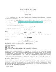
Scarf's algorithm for finding this completely labeled subsimplex is to start in 

the corner of S where there is a subsimplex with boundary vertices with all of 

the labels 2,..., n (see Figure 38.1). If the additional vertex of this subsimplex 

(0,0,1) 

I or2 

2or3 3 3 3 1 or3 

(1, 0, O) (0, 1, O) 

Figure 38.1


has the label 1, then the algorithm stops. Otherwise, it proceeds to a new 

subsimplex with all of the labels 2,..., n. The original subsimplex has two 

faces that have all of these labels. One of them includes the interior vertex. 

The algorithm moves to the unique other subsimplex that shares this face. If 

the additional vertex of this subsimplex has the label 1, the algorithm stops. 

Otherwise, it proceeds, moving to the unique subsimplex that shares the new 

face and has the labels 2,..., n. The algorithm cannot try to exit through a 

boundary face. (Think of what labels the vertices of such a face must have.) 

Nor can it cycle. (To cycle there must be some subsimplex that is the first that 

the algorithm encounters for the second time; but the algorithm must have 

previously encountered both of the subsimplices that share the two faces of this 

subsimplex with the labels 2,..., n.) Since the subdivision consists of a finite 

number of subsimplices, the algorithm must terminate with a completely 

labeled subsimplex. 

To see the connection of this algorithm with Brouwer's theorem, we assign a 

vertex v with a label i for which gi(v) >i v i. Since e'g(v) = e'v = 1, there must 

be such an i. Notice that, since gi(v) >i O, i can be chosen such that the labeling 

convention on the boundary is satisfied. A completely labeled subsimplex has 

vertices v 1 ,...,v n such that g~(vi)>~v~, i i=l,...,n. To prove Brouwer's 

theorem, we consider a sequence of subdivisions whose mesh, the maximum 

distance between vertices in the same subsimplex, approaches zero. Associate 

each subdivision with a point in a completely labeled subsimplex. Since S is 

compact, this sequence of points has a convergent subsequence. Call the limit 

of this subsequence ~. Since g is continuous, we know gi(~)/> xi, i = 1,..., n. 

Since e' g(.f) = e'.f = 1, g(Yc) = ~. 

Scarf does not consider an infinite sequence of subdivisions, which is the 

non-constructive aspect of this proof. Instead, he works with a subdivision with 

a small mesh. Any point in a completely labeled subsimplex serves as an 

approximate fixed point in the sense that II g(x) - xll


this algorithm to situations where g is an arbitrary continuous map and S is 

again the simplex. 

If S has no fixed points, we could define a map 

h(x) = A(x)(x - g(x)) 

where A(x)= ((x- g(x))'(x- g(x))) -1/2. This map would be a retraction of S 

into its boundary: it would continuously map S into OS and be the identity on 

0S. Hirsch proves that no such map could exist, thereby proving Brouwer's 

theorem. Smale proposes starting with a regular value of x- g(x), a point 

£ E 0S such that I - Dg(£) is non-singular. Sard's theorem says that the set of 

regular values has full measure and, in particular, that there exists such a point 

2. The algorithm then follows the solution to 

A(x(t))(x(t) - g(x(t))) = £. 

Since the path x(t) cannot return to any other boundary point, and since it 

cannot return to £ because it is a regular value, it must terminate at a fixed 

point (see Figure 38.2). 

Differentiating the above equation with respect to t, we obtain 

A(x)(l - Dg(x))2 + X(x - g(x)) = O. 

Smale shows that x(t) can be chosen as the solution to the differential equation 

(I - Og(x))x = t~(x)( g(x) - x) 

where /z(x) has the same sign as det[I-Dg(x)] and is scaled so that ~ has 

constant velocity. Except for the factor t~ this is a continuous version of 

Figure 38.2 

5


Newton's method for solving x - g(x) = 0: 

x,+, = x, - (I - Og(xt))-l(x, - g(xt) ) . 

2.4. Regularity and the index theorem 

Merely establishing the existence of equilibria and developing methods for 

computing them leaves important questions unanswered. Are equilibria 

unique? If not, are they locally unique? Do they vary continuously with the 

parameters of the economy? In recent years, economists have used the tools of 

differential topology to investigate these questions. Debreu (1970) has investi- 

gated the questions of local uniqueness and continuity with continuously 

differentiable excess demand functions. See Dierker (1982) and Mas-Colell 

(1985) for surveys of this and subsequent work. Analogous results to those 

derived in the differentiable framework can be obtained in a piecewise-linear 

framework applicable to Scarf's approach to computing equilibria. See, for 

example, Eaves and Scarf (1976) and Eaves (1976). 

Debreu (1970) defines a regular economy to be one that satisfies conditions 

sufficient for there to be a finite number of equilibria. Dierker and Dierker 

(1972) simplify these conditions to the requirement that the Jacobian matrix of 

excess demands_Df(~) with the first row and column deleted, the (n- 1)× 

(n - 1) matrix J, is non-singular at every equilibrium. The first row is deleted 

because of Walras's law, the first column because of homogeneity. We are left 

with a square matrix because, as Wairas (1874, Lesson 12) pointed out, the 

number of equations equals the number of unknowns in the equilibrium 

conditions. The inverse function theorem implies that every equilibrium of a 

regular economy is locally unique. Since the set S is compact and the 

equilibrium conditions involve continuous functions, this implies that a regular 

economy has a finite number of equilibria. 

Let us rewrite the equilibrium conditions as f(p, b) = 0 where b E B and B is 

a topological space of parameters. If f and its partial derivatives with respect to 

p are continuous in both p and b, then the implicit function theorem implies 

that equilibria vary continuously at regular economies. Furthermore, in the 

case where B is the set of possible endowment vectors w i, Debreu uses Sard's 

theorem to prove that, for every b in an open set of full measure in B, f(., b) is 

a regular economy. When B is the function space of excess demand functions 

with the uniform C ~ topology, an open dense set of B consists of regular 

economies. Consequently, if we are willing to restrict attention to continuously 

differentiable excess demand functions, a restriction that Debreu (1972) and 

Mas-Colell (1974) have shown in fairly innocuous, almost all economies, in a 

very precise mathematical sense, are regular. 

2059


Dierker (1972) has noticed that a fixed point index theorem could be used to 

count the number of equilibria of a regular economy. Let us define the fixed 

point index of a regular equilibrium/~ as sgn[det(I- Dg(/~))] whenever this 

expression_is non-zero. Dierker shows that the index can also be written as 

sgn(det[-J]). The index theorem says that ~ index(/~)= +1 where the sum is 

over equilibria of a regular economy. This result is depicted in Figure 38.3 

where n =2, Pl = 1 -P2, and gl(Pl, P2) = 1 -g2(P~, P2). Here index(/~) = 

sgn(1 - Og2/Op2 ) and a regular economy is one where the graph of g does not 

become tangent to the diagonal. 

Mas-Colell (1977) shows that any compact subset of S can be the equilibrium 

of some economy f. If we restrict ourselves to regular economies and n ~> 3, 

then the only restrictions placed on the number of equilibria are those given by 

the index theorem. (If n = 2, an equilibrium with index -1 must lie between 

two with index + 1.) This implies that the number of equilibria is odd and that 

there is a unique equilibrium if and only if index(/~) = +1 at every equilibrium. 

It is easy to see that there are an odd number of solutions to Scarf's 

algorithm and to Smale's global Newton method. To see this in the case of 

Scarf's algorithm, let us argue that there are an odd number of completely 

labeled subsimplices. The path followed from the corner missing the label 1 

leads to a unique subsimplex. Suppose there is an additional completely 

labeled subsimplex. Then it shares the face with labels 2,..., n with a unique 

other subsimplex. Restart Scarf's algorithm at this subsimplex. Either the 

additional vertex to this subsimplex has the label 1, in which case it is 

completely labeled, or it does not, in which case it has another face with all of 

the labels 2,..., n. Move to the unique other subsimplex that shares this face 

and continue as before. The algorithm cannot encounter any subsimplex in the 

O(P) 

0 

Figure 38.3 

P


path from the corner to the original subsimplex. (To do so there must be some 

subsimplex in the path that is the first that it encounters; but it must have 

previously encountered both of the subsimplices that share the two faces of this 

subsimplex with the labels 2,..., n.) The algorithm must therefore terminate 

in yet another completely labeled subsimplex. Consequently, all completely 

labeled subsimplices, except the original one located by the algorithm starting 

in the corner, come in pairs. There is a definition of index of a completely 

labeled subsimplex that agrees with that of a fixed point/~ in the case where the 

mesh of the subdivision is sufficiently small and f is regular [see Eaves and 

Scarf (1976) and Todd (1976b)]. The original subsimplex located by the 

algorithm starting in the corner has index + 1. All other completely labeled 

subsimplices come in pairs as described above, one with index + 1 and one with 

index - 1. 

Likewise, it can be shown that the global Newton method has an odd 

number of solutions. Starting at ~ on the boundary the algorithm locates one, 

which has index + 1. All other solutions are matched up in pairs, one with 

index +1 and one with index -1. Indeed, it is a general feature of these and 

related algorithms that, unless they are restarted at a fixed point different from 

the one originally computed by the algorithm, they always lead to fixed points 

with index +1. This, combined with Mas-Colell's (1977) result about the 

arbitrariness of the number of fixed points, suggests that, unless for some 

reason we know that index(/~)= +1 at every fixed point, there can be no 

method except for an exhaustive search that locates all fixed points. There is an 

important possible exception to this remark involving the all-solutions al- 

gorithm of Drexler (1978) and Garcia and Zangwill (1979, 1981). This method, 

which depends on being able to globally bound g using complex polynomial 

functions, is further discussed in the next section. 

2.5. Path following methods 

Much recent work on the computation of fixed points has been based on the 

idea of path following. The idea is to follow the path of solutions to H(x, O) = 0 

where H : S × [0, 1] ~ R n is chosen so that H(x, 0) = 0 is trivial to solve and 

H(x, 1) = x - g(x), which means a solution to H(x, 1) = 0 is a fixed point. The 

function H is called a homotopy [see Garcia and Zangwill (1981) for a survey 

and references]. 

Suppose that g : S---~ S is twice continuously differentiable. Define 

H(x, O) = x - (1 - 0)Y - Og(x) 

where £ is an interior point of S. Notice that, for any 1 > 0 >/0 and x E S,


(1 - 0)~ + Og(x) is also interior to S. We start at the trivial solution H(£, 0) --- 0 

and follow the solution path until we reach the boundary where 0 = 1 and 

H(x, 1) = x - g(x) = 0. We require that 0 be a regular value of H(x, O) in the 

sense that the n × (n + 1) matrix DH(x, O) has rank n whenever H(x, O) = O. 

Sard's theorem says that we can always choose £ so that this condition is 

satisfied and, indeed, that it is satisfied for almost all £. (It is here that second 

differentiability is important.) The implicit function theorem then implies that 

solutions to H(x, 0) = 0 form a compact one-dimensional manifold with bound- 

ary, a finite number of paths and loops, and that the boundary points of this 

manifold are also boundary points of S × [0, 1]. By construction, H is such that 

(£, 0) is the only possible boundary solution except for points where 0 = 1, 

where solutions are fixed points of g (see Figure 38.4). 

Although the path that starts at (£, 0) cannot return to the boundary where 

0 = 0, it need not be monotonic in 0. Consequently, we do not want to think of 

the path in terms of x as a function of 0. Rather, let us write y(t) = (x(t), O(t)). 

Differentiating H(y(t))=--0 with respect to t, we obtain 

DH(y)~ = O. 

This is a system of n linear equations in n + 1 unknowns that has an infinite 

Figure 38.4 

0


number of solutions. One is 

))i "~" (-1) "-~+~ det DH(y)_~. 

Here DH(y)_ i is the n × n matrix formed by deleting column i from DH(y). 

That 0 is a regular value of H implies that at every point y along the path some 

matrix DH(y)_ i is non-singular. To see that the above differential equation 

does indeed follow the solution path to H(y) = 0, we suppose that DH(y)_I is 

non-singular and rewrite DH))= 0 as 

n+l 

E DiH))i =-D1H))I 

i=2 

where DiH is column i of DH. We choose ))1 ~ (--1) n det DH 1 and solve for 

))2 .... , ))n+l using Cramer's rule: 

.9 = Oet[D2H'" D ~ 1H(-1)n+~(det DH1)DIHDi+~H'" D~+~H] 

+ det DH 1 

= (-1) n-i÷1 det DH_ i . 

As with the global Newton method, we have reduced the problem of 

computing fixed points to that of solving a system of ordinary differential 

equations. To solve such equations, we can use a variety of methods, such as 

the Runge-Kutta method or the Bulirsch-Stoer method [see, for example, 

Gear (1971) and Stoer and Bulirsch (1980, Chap. 7)]. The homotopy approach 

can also be applied to piecewise-linear problems [see, for example, Merrill 

(1971), Eaves (1972), Kuhn and MacKinnon (1975), Eaves (1976) and Eaves 

and Scarf (1976)]. 

The homotopy approach yields a very simple proof of the index theorem. 

Notice that at 07, 0) 

O = det[DH(£, O)_(n+l)] ~-- det I = 1 > O. 

Following the path of solutions to H(x(t), O(t)) = O, O may change signs, but 

when 0 = 1 

O = det[DH(x, 1)_(n+l)] = det[I- Dg(x)] 

must be non-negative. (Takeanother look at Figure 38.4.) If 0 is a regular 

value of x - g(x), if the economy is regular, then det[I- Dg(x)] > 0. Other 

fixed points come in pairs, with each one the endpoint of a path that starts and 

ends on the boundary where 0 = 1. At one endpoint 0 ~< 0 and at the other 

I> 0. In the regular case we define index(~) = sgn(det[I - Dg(~)]). Summing


over all fixed points, all solutions to H(x, 1) = 0, yields +1. This proof of the 

index theorem is easily extended to maps that are continuously differentiable 

only of first, rather than second, order [see Garcia and Zangwill (1981, Chap. 

22)1. 

A fascinating possibility presented by the path following idea is that of being 

able to compute all of the fixed points of a function g : S--> S. The all-solutions 

algorithm of Drexler (1978) and Garcia and Zangwill (1979) is easiest under- 

stood in terms of computing zeros of polynomials. We first approximate 

g(x) - x by a finite order polynomial f : S---~ R" and then extend fto a function 

f : R"--> R n. Weierstrass's approximation theorem says that we can choose f to 

approximate g(x) - x arbitrary closely on S [see, for example, Lang (1983, pp. 

49-53)]• We then convert f into a complex function by allowing both its 

domain and range to be C n, the space of complex n vectors. We can expand the 

, - , .~_ 

vector z E C n into a vector z* E R 2n by writing z =(z~ + Zzl,..• , Z2n 1 

Z~ni). Consequently, we can expand f into f* : RZn---> R 2n by writing f(z) = 

(f~(z*) + • /2\ ~*tz*li ] '" .., f2, * 1( z * ) + f2n(Z * * )t). " We now discuss a method that 

can compute all the zeros of f*. Notice that not all of the zeros of f* are 

approximate fixed points of g; some may be complex and some may lie outside 

of S. 

Letting rnj be the highest order of the polynomial fj(z), we consider the 

homotopy H : C n × [0, 1]--> C ~ defined by the rule 

Hj(z,O)=(1-O)(z~ 'n'+')- l)+Ofj(z), ]=1 .... ,n. 

At 0 = 1, solutions to H(z, 0)= 0 are zeros of f. At 0 = 0, Hi(z, 0)= 0 has 

m i + 1 solutions 

zj = cos(21ra/(mj + 1)) + i sin(2~a/(mj + 1)), a - 0, 1 ..... rnj . 

n + 

Consequently, there are IIj= 1 (rnj 1) solutions to H(z, 0) = 0. We can expand 

• , 

H into H 

2n 

: R 

~ 

× [0, 1] 

2n 

R . The crucial insight involved in the all-solutions 

algorithm is that any solution path to H*(z*, 0) = 0 is monotonic in 0, 

0 = det[DH*(z*, 0)_(2n+1) ]/> 0. 

The 

[ 

proof is simple: DH*(z*, 0)_(2,+1) consists of 2 × 2 blocks of the form 

oH oH ] 

o-i oHl l


r i r 

Here zj = z~j_ 1 is the real part of zj, zj = z~. is the imaginary part, and H i and 

H i are the real and imaginary parts of H i. The Cauchy-Riemann equations, 

which follow easily from the chain rule, say that 

OHT_ OHI OHT_ OHI 

oz; oz', ' 

Consequently, the 2 × 2 blocks that make up DH*(z*, 0)_(2n+l) all have the 

special form 

aij bij] 

-bij aqj" 

These matrices have important properties: their special form is preserved when 

such a matrix is multiplied by a scalar or inverted; it is also preserved when two 

such matrices are added or multiplied together. Consequently, performing 

Gaussian elimination on these 2 x 2 blocks, we can reduce the 2n × 2n matrix 

DH*(z*, 0)_(2n+l) to a lower block triangular matrix with n such 2 x 2 blocks 

on the diagonal. The determinant is the product of the determinants of these 

blocks, each of which is non-negative. 

Since 0 is monotonic along any path, there can be no paths that both start 

and end at 0 = 0 or at 0 = 1. To guarantee that every solution at 0 = 1 is the 

endpoint of a path that starts with 0 = 0, we need to rule out paths diverging to 

infinity for 0~ (1 - 0). Consequently, Hi(z, O) = 0 

cannot hold for any path along which Ilzll--, ~ and 0 ~< 0 < 1. Following each of 

the paths that starts at 0 = 0 either leads to a zero of f or diverges to infinity at 

0 = 1. No path can start at 0 = 1 and diverge to infinity going backwards, 

however, so this method necessarily locates all of the zeros off [see Garcia and 

Zangwill (1981, Chap. 18) for further discussion]. 

This method can easily be applied to functions other than polynomials. What 

we need is a function f : R'---->.R" than can be extended to C" and polynomials 

(zqi-1) such that some f~(z)/(zq'-l)--->O as Ilzll--'~. The all-solutions 

algorithm is obviously a promising direction for future research. 

2.6. Multiplicity of equilibria 

By constructing an example of an economy with an equilibrium with index -1, 

we can easily construct an example of multiplicity of equilibria.


Example 2.1. Consider a static exchange economy with two consumers and 

two goods. Consumer i, i = 1, 2, has a utility function of the form 

2 

Ui(X1, X2) 2 i, b, _ 1)/bi 

= ajl, xj 

j=l 

where aj i ~ 0 and b i < 1. This is, of course, the familiar constant-elasticity-ofsubstitution 

utility function with elasticity of substitution ~i = 1/(1 - b;). Given 

an endowment vector (wil, w2), i consumer i maximizes this utility subject to his 

budget constraint. His demand functions are 

2 

i i 

"Y j Z pkWk 

xij(pl P2) = k=l i -= 1, 2, j = 1 2 

2 , ~ " 

p~i Z ilrli 

YkPk 

k=l 

Here 7ii = (a'y j. The two consumers have the (symmetric) parameters given 

below. 

Commodity 

Consumer 1 2 

1 1024 1 

2 1 1024 

w; 

b I = b 2 = -4, 

Commodity 

Consumer 1 2 

l 12 1 

2 1 12 

1 2 1 2 

Of course "ql =72 = 1/5, Yl = Y2 =4 and Y2 = Yl = 1. 

This economy has three equilibria, which are listed below. 

Equilibrium 1: pl = (0.5000, 0.5000) 

Commodity 

Consumer 1 2 u i 

1 10.400 2.600 -0.02735 

2 2.600 10.400 -0.02735


Equilibrium 2:p2 = (0.1129, 0.8871) 

Commodity 

Consumer 1 2 u~ 

1 8.631 1.429 -0.10611 

2 4.369 11.571 -0.01497 

Equilibrium 3:p3 = (0.8871, 0.1129) 

Commodity 

Consumer 1 2 u~ 

1 11.571 4.369 -0.01497 

2 1.429 8.631 -0.10611 

This example has been constructed by making p~ = (0.5, 0.5) an equilibrium 

with index - 1 

3.2 -3.2 ] 

"~'Jt/~') '~'- : -3.2 3.2 ' 

index( p l ) = sgn(-3.2) = - 1. 

Remark. A similar example has been constructed in an Edgeworth box 

diagram by Shapley and Shubik (1977). 

Two assumptions have played significant roles in discussions of uniqueness of 

equilibria since the time of Wald (1936). They are gross substitutability and the 

weak axiom of revealed preference. Gross substitutability says that, if p/> q 

and Pi =- qi for some i, then f/(p) >~f,(q) and, if f(p) = f(q), then p = q. (This 

actually combines the two conditions often known as weak gross substitutabili- 

ty and indecomposability.) The weak axiom of revealed preference says that if 

p'f(q) ~ 0 and q'f(p) ~< 0, then f(q) = f(p). 

The argument that gross substitutability implies uniqueness is easy: Suppose 

that there are two vectors p, q, such that f(p) = f(q)~ 0. It must be the case 

that p, q > 0. Otherwise, for example, pg = 0 and 2p ~> p would imply f/(2p) > 

f/(p), which would contradict homogeneity. Let ,/=max qJpj. Then ,/p 

satisfies ,/p >t q, ,/Pi = qi some i. Consequently, f(,/p) = f(p) = f(q) = 0 implies 

,/p = q. It is also easy to show that, when f is continuously differentiable, gross 

substitutability implies that index(/~) = + 1, since 0fi(/~) / Opj >I O, i ~ j implies, 

in general, that -J is a P matrix, a matrix with all of its leading minors positive 

[see Hahn (1958) and Kehoe (1985b)]. 

The weak axiom implies that the set of equilibria is convex. If f is regular, 

this implies that it has a unique equilibrium. Suppose that there are two vec- 

tors p,q such that f(p)=f(q)~O. Then p(O)=Op+(1-O)q, 0~


satisfies p(O)'f(p) O, 

otherwise q'f(p(O)) 0 unless p =/~ and that 

L( p) = ( p - ~)'1~ = -Yfl P) .


Unless p is an equilibrium, f(/3)= 0 and the weak axiom imply that L(p)< O. 

Arrow, Block and Hurwicz (1959) further argue that gross substitutability 

implies that the weak axiom holds in comparisons with an equilibrium vector of 

an exchange model; that f(/3) = 0 implies yf(p) > 0 unless f(p) = f(/3). Con- 

sequently, tfitonnement is also globally asymptotically stable if f satisfies gross 

substitutability. 

If, however, f does not satisfy the weak axiom or gross substitutability, the 

tfitonnement process may not converge to an equilibrium. In fact, Scarf (1960) 

constructs a simple example with unique equilibria in which, unless p(0)= ,6, 

the process converges to a limit cycle. Indeed, the Sonnenschein-Mantel- 

Debreu result on the arbitrary nature of aggregate excess demand implies that 

the behavior of tfitonnement is also arbitrary. See Hahn (1982) for a survey of 

results related to tfitonnement. From our point of view there are two points 

worth noting. First, the process can be generalized to allow different adjust- 

ment speeds 

/ii = 0if~(p) , i=1 .... ,n. 

For any 0 i > 0, i = 1,... , n, the process remains globally stable iff satisfies the 

weak axiom or gross substitutability. In general, however, changing the weights 

0 i can greatly affect the stability properties of t'~tonnement. Second, if we want 

to avoid problems with negative prices we have to alter the process to 

something like 

/ii =/fi(P)[o if pi>0 or fi(p) >0, 

otherwise. 

Although/i can be discontinuous at a point where Pi = 0, it can be shown, as 

done for example by Henry (1972, 1973), that the path p(t) is continuous. 

Van der Laan and Talman (1987) have developed a tfitonnement-like 

algorithm that is guaranteed to converge under weak regularity assumptions: 

start with an initial price vector/~ interior to the simplex. The algorithm sets 

pj/fij = min[p,/fi,,..., P,/fi, l if fj(p) < 0, 

PJ/fii=max[pl//)l,''', P,/fin] iffj(p)>0. 

When fj(p) = O, pj is allowed to vary to keep market j in equilibrium. The set 

of points that satisfy these conditions generically form a collection of loops and 

paths in S. The algorithm operates like the global Newton method and the path 

following methods described earlier, following the path that starts at fi until 

another endpoint is reached. This endpoint is an equilibrium.


Walras (1874, Lessons 12 and 24) originally conceived of tfitonnement as 

clearing one market at a time. With linear equations the analogous process is 

called the Gauss-Seidel method. The idea is to update a guess at a solution to 

the equations 

fj(l, P2, P3 .... , Pn) = 0, j = 2,... , n 

one equation at a time: Given the guess p2k,..., p~, we let p/~+~ be the 

solution gi(p k) to 

f~(1 gz(pk),., g,(pk), k k 

, ", Pi+~,''',Pn)=O, i=2,...,n. 

In the case where f is linear, this method converges if there exists some Oj > O, 

j = 2,..., n, such that 

oi >~ , i,]=2 .... ,n, 

OPi j:~i Opj 

with strict inequality some i [see Young (1971) for a collection of conditions 

that guarantee convergence of this method]. This, however, is the familiar 

diagonal dominance condition satisfied by the Jacobian matrix of an excess 

demand function that exhibits gross substitutability. Consequently, it is pos- 

sible to show that, if Df(~) satisfies gross substitutability at some equilibrium 

/~, there is some open neighborhood N of/~ such that if p0 C N, the non-linear 

analog of this algorithm converges to/~. The weak axiom does not guarantee 

diagonal dominance, and it is easy to construct examples that satisfy the weak 

axiom but for which this method is unstable. 

Perhaps the most popular method for solving systems of equations such as 

g(p) =p is Newton's method, 

p k =p k-l_Ak(/_Dg(pk-1)) l(pk-l_g(pk-~)). 

Frequently, the scalar A k > 0 is chosen by a line search to make ]] pk _ g(pk)]] 

as small as possible. Furthermore, the elements of Dg are usually approxi- 

mated numerically rather than calculated analytically. In many versions of this 

algorithm I- Dg is never explicitly inverted. Rather, an approximation to its 

inverse is successively updated; these are called quasi-Newton methods. See 

Ortega and Rheinboldt (1970) and Jacobs (1977) for surveys of these methods. 

An important warning is in order here: Most work in the mathematical 

programming literature on Newton-type methods relates to minimizing a 

convex function h : R n---~ R,


x k = x k-1 _ AkD2h(xk-1)Dh(xk-1) , . 

Although this does amount to solving the system of equations Dh(x) = 0, this 

system has two special properties. First, D2h is symmetric and positive 

semi-definite. Second, A k can always be chosen small enough so that h(x k) 

decreases at every iteration. Unless I- Dg satisfies strong integrability condi- 

tions, these sorts of properties do not carry over to solving for equilibria. 

Arrow and Hahn (1971, Chapter 12) have shown that a continuous version 

of Newton's method 

t~ = - (I - Dg( p))- '( p - g(p)) 

is globally stable if det(I- Dg(p)) never vanishes. (We ignore the minor 

technical problem caused by the potential discontinuity of Dg; as in the case of 

t~tonnement where some price is zero, p(t) can be shown to follow a 

continuous path.) In this case, the index theorem implies that there is a unique 

fixed point /~ =g(/~). L(p)= ½(p-g(p))'(p-g(p)) provides a Liapunov 

function: L(p)>0 unless p = g(p), and 

L(p) = (p - g(p))'(l - Dg(p))15 = -(p - g(p))'(p - g(p)) . 

Consequently, L(p) < 0 unless p =/3. 

Although this method may cycle if (I- Dg(p)) is singular for some p, L(p) 

always serves as a local Liapunov function near a regular equilibrium/~. That 

is, every regular equilibrium/3 has some open neighborhood N such that, if 

p(0) E N, this method converges to/L This suggests a stochastic method for 

computing equilibria, which is frequently used in practice: Guess a value for 

p(0). Apply Newton's method. If it does not converge, guess a new value for 

p(0). Continue until an equilibrium is located. Since every open neighborhood 

of an equilibrium occupies a positive fraction of the volume of the price 

simplex, this method must eventually work. 

Newton's method is in some sense the simplest algorithm that has this local 

convergence property for any regular equilibrium. Saari and Simon (1978) and 

Traub and Wozniakowski (1976) show that, in a precise sense, any locally 

convergent method must use all of the information in g(p_) and Dg(p). 

Furthermore, Saari (1985) shows that for any step size A k/> A > 0, there are 

examples such that a discrete version of Newton's method is not even locally 

convergent. Since we cannot always choose A k so that lip- g(p)ll is decreas- 

ing, we have to bound A~ from below so the method does not get stuck away 

from an equilibrium. Saari shows that this may result in the method overshoot- 

ing the equilibrium.


Notice that the global Newton method has a global convergence property. It 

uses global information, however, because it is only guaranteed to work if 

started on the boundary or at an equilibrium with index -1. Otherwise, it may 

cycle [see Keenan (1981)]. Notice too that the global Newton method diverges 

from any equilibrium with det[l-Dg(/3)]


o~,u,(x'(,~)) + p' ~ (w'- x'(o~)) 

i=l i=l 

E + E (w'- 

i=1 i=1 

>t ~ aiui(x') + p(a)' ~ (w'- x') 

i=1 i=1 

for all p~>0 and (xl,... ,xm)~>0. 

Similarly, each consumer solves his utility maximization problem in equilib- 

rium if and only if there exists Ai ~> 0 such that 

u,(i') + a,p'(w' fc') >1 u,(, i) + ~,p'(w' ~' > ' 

- - x ) ~ ui(x ) + i,p'(w' - x') 

for all A~ 1> 0 and xi~ O. Notice that the strict monotonicity of ui implies that 

A~ > O, otherwise we would violate the second inequality simply by increasing 

x i. Dividing the second inequality through by '(i and summing over i-- 

1,..., m produces 

E ~' E - E (1 /,X~)u,(x ) ~ (w' - x') 

i~l i=1 i=l i=1 

for all (x 1 .... , x m) >i O. Moreover, since ,3' Xi~ 1 (w' - 2') = 0 because of strict 

monotonicity and E i~ 1 (w' - ~')/> 0 because of feasibility, 

i~l i=1 i=1 i=1 

for all p/> 0. Consequently, every competitive equilibrium solves the above 

Pareto problem where a~ = 1/A i, i= 1 ..... m and p(a)=ft. This can be 

viewed as a proof of the first welfare theorem. 

Notice, too, that, if (xl(a),..., xm(a)) is a solution to the Pareto problem 

for arbitrary non-negative welfare weights a, it must be the case that 

i 

~,u,(x (~)) + p(~)'(x'(~) - 2(~))/> ~,u,(x') + p(~)'(x'(,~) - x ~) 

for all xi~ 

> O. Otherwise the allocation that replaces xi(a) with the x g that 

violates this inequality but leaves xJ(a), j # i, unchanged would violate the 

conditions required for (if(cO,... , xm(a)) to solve the Pareto problem. Since 

p'(ff(a)- xi(a))= 0 for all p, this implies that any solution to the Pareto 

problem is such that, if a i > O, xi(a) maximizes ui(x ) subject to p(a)'x


(xl(a),... ,xm(ol)) as an equilibrium with transfer payments ti(a)= 

p(a)'(xi(a) - wi), i = 1,..., m. 

Suppose now that ot i = 0, some i. Then our earlier argument implies 0 ~> 

p(a)'(x~(a)-x ~) for all x~>~0. Combined with p(a)>~O, this implies that 

p(a)'xi(a) -- 0, that consumers with zero weight in the welfare function receive 

nothing of value at a solution to the Pareto problem. Since the strict monoto- 

nicity of ug implies p(a) ~ 0 and since w ~ > 0, we know that te(a ) > 0 if a i = 0. 

Our arguments have produced the following characterization of equilibria. 

Proposition 3.1. A price-allocation pair (/3, ~l,...,.f,,) is an equilibrium if 

and only if there exists a strictly positive vector of welfare weights (&l, • • • , &m) 

such that (£c I, . . . , fc m) solves the Pareto problem with these welfare weights, that 

/3 is the corresponding vector of Lagrange multipliers, and that/3'(~i _ w i) = O, 

i=1,... ,m. 

Remark. The assumption that w i is strictly positive serves to ensure that the 

consumer has strictly positive income in any equilibrium and, hence, has a 

strictly positive welfare weight. Weaker conditions such as McKenzie's (1959, 

1961) irreducibility condition ensure the same thing. Unless there is some way 

to ensure that the consumer has positive income, or, with more general 

consumption sets, can afford a consumption bundle interior to his consumption 

set, we may have to settle for existence of a quasi-equilibrium rather than an 

equilibrium. In a quasi-equilibrium each consumer minimizes expenditure 

subject to a utility constraint rather than maximizing utility subject to a budget 

constraint. 

Unless we are willing to assume that ui, i= 1,..., m, is continuously 

differentiable, there may be more than one price vector p(a) that supports a 

solution to the Pareto problem because of kinks in u i. This makes t(a) a 

point-to-set correspondence. Nevertheless, it is still easy to prove the existence 

of equilibrium using an approach due originally to Negishi (1960). 

Proposition 3.2 [Negishi (1960)]. There exists a strictly positive vector of utility 

weights (dq, . . . , &m) such that 0 E t(&). 

Proof. The strict concavity of each ui, i= 1,..., m, and continuity of 

Z m aiUi(X i) in a implies that x z R" 

i=1 :R+\{O}---~ is a continuous function. 

Furthermore, p:R+\{0}---~R n is a non-empty, bounded, upper-hemi-con- 

tinuous, convex-valued correspondence. Consequently, the correspondence 

t : R+\{0}--~ R m defined by the rule 

= - w


is also non-empty, bounded, upper-hemi-continuous and convex-valued. It is 

homogeneous of degree one since xi(a) is homogeneous of degree zero and 

p(a) is homogeneous of degree one. It also obeys the identity 

2 ti(a)~p(a)' ~ (xi(Ol) -- Wi)~--0. 

i=1 i~l 

Let S C R m now be the simplex of utility weights. Since S is compact, t is 

bounded and upper-hemi-continuous and ti(a ) < 0 if a E S with a i = O, there 

exists 0 > 0 such that 

g(a) -- a - Ot(a) 

defines a non-empty, upper-hemi-continuous, convex-valued correspondence 

g" S---~S. By Kakutani's fixed point theorem there exists & ~g(&). This 

implies that 0 E t(3). 

Remark. The correspondence f : R+\{O}--~R m defined by the rule 

f(a) = - ti(a )/a i has all of the properties of the excess demand correspondence 

of an exchange economy with m goods. 

3.2. Computation and multiplicity of equilibria 

Negishi's approach provides an alternative system of equations a = g(a), that 

can be solved to find equilibria. Mantel (1971), for example, proposes a 

tfitonnement procedure & =-t(a) for computing equilibria. Similarly, we 

could apply Scarf's algorithm, the global Newton method, a path following 

method, the non-linear Gauss-Seidel method, or Newton's method to compute 

the equilibrium values of a. 

We have reduced the problem of computing equilibria of an economy 

specified in terms of preferences and endowments to yet another fixed point 

problem. The obvious question, in analogy to Uzawa's (1962) result, is 

whether any arbitrary g:S----~S, S C R m can be converted into a transfer 

function t(a). The answer is obviously yes if the only properties that t needs to 

satisfy are continuity, homogeneity of degree one and summation to zero. 

Bewley (1980), in fact, proves the analog of the Sonnenschein-Mantel-Debreu 

theorem is the case where t is twice continuously differentiable and n i> 2m: for 

any such transfer function t there is an economy with m consumers and n goods 

that generates it. In closer analogy with the Sonnenschein-Mantel-Debreu 

theorem, however, it is natural to conjecture that this result holds for t 

continuous and n/> m.


Example 3.1 (2.1 revisited). The Pareto problem for the exchange economy 

with two goods in Example 2.1 is 

2 2 

~'~ 1/," 1 xb 

max ffl Z., ajttxj) - 1)/b + c~ 2 ~, ajttx~)2" 2,b _ 1)/b subject to 

j=l j=1 

1 _1_ X~ ~ 1 ...]_ 2 

xj w i w~, j=l,2, 

Xj ~>0 

(It is only in the case b~ = b 2 that we can obtain an analytical expression for the 

transfer functions.) The first-order conditions for this problem are 

il ixb-1 

otia/[xj) -- pj = O, i = 1, 2, j = 1, 2. 

These are, of course, the same as those of the consumers utility maximization 

problem when we set ai = 1/A~. The difference is that here the feasibility 

conditions are imposed as constraints, and we want to find values of a i so that 

the budget constraints are satisfied. In the previous section the budget con- 

straints were imposed as constraints, and we wanted to find values of pj so that 

the feasibility constraints were satisfied. 

The solution to the Pareto problem is 

: 

2 

(aiaij) n ~ w~ 

2 

2 (aka~) n 

k=l 

, i=1,2, j=l,2. 

Here, once again, 7/= 1/(1 - b). The associated Lagrange multipliers are 

pj(o,) = 

Equilibria are now solutions to the equation 

ti(oq, a2) = p(a)'(xi(a) - w i) = O, i = 1, 2. 

Since tl(a)+ t2(a)-----0 , we need only consider the first equation. Since t I is 

homogeneous of degree one, we can normalize a~ + ot 2 = 1. There are three


solutions, each of which corresponds to an equilibrium of Example 2.1. They 

are a I = (0.5000, 0.50000), a 2 = (0.0286, 0.9714) and a 3 = (0.9714, 0.0286). 

In some cases equilibria solve optimization problems that do not involve 

additional constraints like ti(a ) = 0. Two notable cases are (1) where utility 

functions are homothetic and identical but endowments arbitrary and (2) 

where utility functions are homothetic but possibly different and endowment 

vectors are proportional. In the first case, considered by Antonelli (1886), 

Gorman (1953) and Nataf (1953), the equilibrium allocation (~1 ..... ~m) 

maximizes U(~im=l X') subject to feasibility conditions; here u is the common 

utility function. In the second case, considered by Eisenberg (1961) and 

Chipman (1974), the equilibrium allocation maximizes Eim~ 0; log ui(xi); here 

u~ is the homogeneous-of-degree-one representation of the utility function and 

0 i is the proportionality factor such that w ~= 0 i Zjm=l W j. 

The characterization of equilibria as solutions to optimization problems is 

useful to the extent to which it is easy to find the optimization problem that an 

equilibrium solves. The Negishi approach is useful in situations in which the 

number of consumers is less than the number of goods and the Pareto problem 

is relatively easy to solve. 

It is worth noting that there is always a trivial optimization problem that an 

equilibrium (~,/)) solves: 

min(llx - £[l 2 + lip -/3ll2) • 

The only way that we can find this problem, however, is to compute the 

equilibrium by some other means. Another point worth noting is that the 

Pareto problems that we have considered are convex problems, which have 

unique solutions that are easy to verify as solutions and relatively easy to 

compute. Any fixed point problem, and hence any equilibrium problem, can be 

recast as an optimization problem, 

mini[ p - g(p)[[ 2 . 

Because the objective function is not convex, however, it is relatively difficult 

to compute equilibria using this formulation. Nevertheless, this problem does 

have one aspect that makes the solution easier than that of other non-convex 

optimization problems: Although we may possibly get stuck at a local mini- 

mum, at least we know what the value of the objective function is at the global 

minimum, II/~ - g(/))l[ 2 = o. 

A recent development that may allow efficient solution to non-convex 

optimization problems is the simulated annealing algorithm. This algorithm, 

developed by Kirkpatrick, Gelatt and Vecchi (1983), is based on the analogy


between the simulation of the annealing of solids and the solution of combina- 

tional optimization problems [see van Laarhoven and Aarts (1988) for a survey 

and references]. Although this method has been applied principally to com- 

binatorial problems, which involve discrete variables, there have been some 

applications to continuous optimization problems (see, for example, Vanderbilt 

and Louie (1984) and Szu and Hartley (1987)]. So far, this method has not 

been applied to solve economic problems, however, and it remains an intrigu- 

ing direction for future research. 

4. Static production economies 

We can add a production technology to our model in a variety of ways. Perhaps 

the easiest, and in many ways the most general, is to specify the production 

technology as a closed, convex cone Y C R n. If y @ Y, then y is a feasible 

production plane with negative components corresponding to inputs and 

positive components to outputs. We assume that -R+ C Y, which means that 

n 

any good can be freely disposed, and that Y 91 R+ = {0}, which means that no 

outputs can be produced without inputs. 

The production cone specification assumes constant returns to scale. With 

the introduction of fixed factors, it can also account for decreasing returns. It 

cannot account for increasing returns, however, which are not compatible with 

the competitive framework that we employ here. See Chapter 36 for a survey 

of results for economies with increasing returns. 


In an economy in which consumers are specified in terms of utility functions 

and endowment vectors, an equilibrium is now a price vector/) E R+\{0}, an 

allocation (~,... , :fro), where ~ E R~, and a production plan 3~ E Y such that 

• x, /=1,... ,m, solves 

max ui(x ) subject to/)'x


• /)'y~~O,j=l,...,k . 

j=l 

For example, h(Zl,Z2, z3)='O(-Zl)°(-z2) 1 °--Z 3 is the familiar Cobb- 

Douglas production function. (Of course, the activity analysis specification 

is a special case of this one since, for example, h(zl, z 2, z3) = min[-zl/au, 

--z2/a2j ] -- z3/a3j is a concave production function.) 

Another alternative is to allow decreasing returns to scale, where the 

production function hi is strictly concave. In this case, the problem of maximizing 

p'z subject to hi(z)>~ 0 has a unique solution zJ(p). Unless z](p) = 0 there 

are positive profits 7r](p)=p'zJ(p) that must be spent. Letting 0~>~0, 

Em 

i=~ 0i 

i 

--- 1, j = 1 ..... k, be profit shares, we change the budget constraint of 

consumer/to p'x


Consider the set 

S r={PER "le'p=l,p'y


passing through g with normals (g(p) -p -f(p)) separates g(p) from Sy. If 

(p + f(p)) E St, then g(p)=p + f(p) and the inequality is trivial. 

Suppose that /3 =g(/3). Then the above inequality becomes q'f(/3)


functions. Let at(p) be the restricted profit corresponding to the production 

function hi(z), the value of the objective function at the solution to 

max p'z subject to ht(z ) >! O, Ilzll = 1. 

(For production functions with only one output i a restriction like z i= 1 is 

more natural than Ilzll = 1.) if this problem has a unique solution zt(p), then 

at(p) is continuously differentiable and, by Hotelling's lemma, Dat(p)= 

zt(p) ' [see, for example, Diewert (1982)]. In this case g(p) is found by solving 

min ½(g-p-f(p))'(g-p-f(p)) subject to 

at(g)


Once again, if f satisfies the weak axiom, the set of equilibria is convex, and 

in the regular case there is a unique equilibrium. Unfortunately, even if f 

exhibits gross substitutability, the economy need not have a unique equilib- 

rium, as the following example illustrates. 

Example 4.1. Consider a static production economy with two consumers and 

four goods. Consumer i, i = 1, 2 has a utility function of the form 

Ui(X 1 , X 2, X 3, X4) 2 aij log x~ 

j=l 

4 

• i i i 

where a'j i> 0. Given an endowment vector (wi~, w2, w3, w4), consumer i maxi- 

mizes this utility function subject to his budget constraint. The aggregate excess 

demand function is 

£(Pl' Pe' P3' P4)= ~(i=I 

4) 

i ~ pkWik 

aj k=l 

4 

i 

Pj ~ ak 

k=l 

The consumers have the parameters given below. 

Commodity 

j=1,2,3,4. 

Consumer 1 2 3 4 

1 O.8 0.2 0 0 

2 0.1 0.9 0 0 

w'j 

Commodity 

Consumer 1 2 3 4 

1 0 0 10 0 

2 0 0 0 20 

The production technology is specified by a 4 x 8 activity analysis matrix 

A = 

-1 0 0 0 3 5 -1 -1_!]] 

0 -1 0 0 -1 -1 5 

0 0 -1 0 -1 -1 -1 " 

0 0 0 -1 -1 -4 -3 

(The first four columns are disposal activities.)


This economy has three equilibria, which are listed below together with the 

welfare weights for which the corresponding Pareto problem yields the same 

equilibrium. 

Equilibrium 1: 

pl= (0.2500,0.2500,0.2500,0.2500), 

yl= (0,0,0,0,5.00000,0,5.0000,0), 

a 1= (0.3333,0.6667). 

Commodity 

Consumer 1 2 3 4 u i 

1 8.000 2.000 0 0 1.8022 

2 2.000 18.000 0 0 2.6706 

Equilibrium 2: p2 = (0.2500,0.2222,0.3611,0.1667), 

y~=(0,0,0,0,5.1806,0.3611,4.4583,0), 

a = (0.5200,0.4800). 

Commodity 

Consumer 1 2 3 4 ui 

1 11.555 3.250 0 0 2.1935 

2 1.333 13.500 0 0 2.3719 

Equilibrium 3: 

p~=(0.2500,0.2708,0.1667,0.3125), 

Y3 (0, 0, 0, 0, 4.3690, 0, 5.1548, 0.1190), 

a (0.2105,0.7895). 

Commodity 

Consumer 1 2 3 4 u i 

1 5.333 1.231 0 0 1.3807 

2 2.500 20.769 0 0 2.8217 

This example has been constructed by making pl = (0.25, 0.25, 0.25, 0.25) be 

an equilibrium with index (pl)= -1. 

-40 0 32 

,, o -8o 8 

/-/J~// I 0 0 0 

0 0 0 

{ [800 

index(p~) = sgn |det | 0 

\ 

index( p l ) = sgn(-416) = - 1. 

72 

8 7 2 1 

0 0 -1 -1 

0 0 -1 - 

1 1 0 

0 3 0


That this example has multiple equilibria means that gross substitutability 

does not imply the weak axiom. Kehoe and Mas-Colell (1984) prove that gross 

substitutability does indeed imply the weak axiom if n ~< 3, so at least four 

goods are needed for this example. Kehoe (1985b) presents an example with 

multiple equilibria in which the f exhibits strong gross substitutability, 0f~/ 

Opj > 0. The simple form of a Jacobian matrix in this example, which satisfies 

gross substitutability but implies a violation of the weak axiom is due to 

Mas-Colell (1986) [see also Hildenbrand (1989) and Kehoe (1986)]. 

Unfortunately, as Herbert Scarf has demonstrated to the author, the weak 

axiom is the weakest condition on f that guarantees that a production economy 

has a unique equilibrium. Suppose that there are two distinct price vectors p 

and q such that p'f(q)~< 0 and q'f(p)

2086 TJ. Kehoe 

Lagrange multipliers y such that 

q-f(p)+ B(p)y=O, y@'(p)q=O. 

At q = 0 this becomes f(/)) =/~(/~)y. 

Let B(p) be the n x I submatrix of/~ whose columns are associated with 

strictly positive Lagrange multipliers. Then we can solve explicitly for q to 

obtain 

D = (I - B(p)(B'(p) B(p))- 1B '( p))fl p). 

Like the tfitonnement process for exchange economies, this process leaves ]l P 11 

constant. Also like the tfitonnement process for exchange economies, this 

process is globally asymptotically stable if the weak axiom of revealed prefer- 

ence holds in comparisons between arbitrary price vectors p and the equilib- 

rium price vector/~. Suppose that p ~ Y*. Then f(/3) ~ Y implies p'f(fi)


reduction in dimension of this sort to carry out exhaustive searches to verify 

that two large-scale applied general equilibrium models have unique equilibria. 

We begin with the activity analysis case. A production economy (f, A) has a 

generalized input-output structure if it satisfies the following conditions: 

• There are h 0 such that 

m 

Ej~ aj/>O, i=1 .... ,n- h. 

• Every good that can be produced is actually produced at every equilibrium. 

To ensure that this final condition holds, we could require that fg(p)~>0, 

i = 1,..., n - h, for all p or, what is almost the same thing, that consumers 

have no endowments of produced goods. In the case where h = 1 these 

conditions are those of the non-substitution theorem [see Samuelson (1951)]. 

Let p E R n-h now be the vector of prices of produced goods and q E R h be 

the vector of factor prices. Partition A into 

[A:] 

where A~ is (n-h) × k and A 2 is h × k. Similarly, partition f(p, q) into 

(f~(p, q), f2(p, q)). 

In the case where A consists of 2n - h activities, n disposal activities and an 

n × (n - h) matrix B with .one activity to produce each of the produced goods, 

the reduction of the search to the space of factor prices is easy. Our 

assumptions imply that the (n - h) × (n - h) matrix Ba is a productive Leontief 

matrix. Under a mild indecomposability assumption, B~ -~ is strictly positive. 

The equilibrium condition B133 =fl(/~, q) implies that )3 = B~-lfl(/~, q), and 

the zero profit condition/~'B~ + 4'B 2 = 0 implies that/~ = -(B2Bl-1)'4 . We are 

left with the equilibrium condition B2~ =f2(/% 4). We define the function 

q," Rh+\ {0} ~ R h by the rule 

~b(q) =f2(-(B2Bl')'q, q) - B2B ~f'(-(B2Bl')'q, q). 

It is easy to verify the ~0 is continuous, is homogeneous of degree zero and 

obeys Walras's law because f satisfies these properties. Notice that ~0(q) = 0 is 

equivalent to 

f2(/~, q) = B2B?' fl(P, 4) = B2f~. 

Consequently, 4 is an equilibrium of the h-good exchange economy qJ is and 

only if (/~, q) is an equilibrium of the n-good production economy (f, A).


When there is more than one possible activity for producing each good the 

situation is slightly more complicated. To calculate qJ(q) we start by solving the 

linear programming problem 

min -q'Azy subject to A~y = e, y >~0. 

Our assumptions imply that this problem is feasible and has a finite maximum. 

The non-substitution theorem says that the solution is associated with a feasible 

basis, 

-q'B2] 

B, J~ 

that is, a matrix of n - h columns associated with positive activity levels yj that 

does not vary as the right-hand side varies, although the activity levels 

themselves do. Furthermore, there is a vector of prices p such that p'B~ + 

q'B 2 = 0 and p'Aa + q'A 2 40 [see Gale (1960, pp. 301-306)]. When the basis 

is uniquely defined, we can proceed as above. 

There may, however, be more than one feasible basis possible in the 

solution. Although the linear programming problem may be degenerate, the 

economy itself need not be. Such is the case in Example 4.1, where the 

economy has this generalized input-output structure with n = 4 and h = 2. At 

two of its three equilibria, this example has 3 >2 = n- h activities in use. 

When there is more than one feasible basis possible, the demand for factors 

becomes a convex-valued, upper-hemi-continuous correspondence; 0 E qJ(O) is 

then the equilibrium condition [see Kehoe (1984) for details]. 

With more general production technologies, the situation is similar to the 

activity analysis case with many activities. For any vector of factor prices q we 

find the cost minimizing production plan for producing an arbitrary vector, say 

e, of produced goods. This plan is associated with a vector of prices p(q), 

which can be plugged into the demand function f l to find the production plan 

that satisfies the feasibility condition in the produced goods markets. This 

production plan induces a demand for factors of production. We systematically 

vary q to make the excess demand for factors equal zero. 

The transformation of an economy with production into an exchange 

economy in factors is also useful for developing conditions sufficient for 

uniqueness of equilibrium. If q, satisfies the weak axiom of revealed preference 

or gross substitutability, for example, then there is a unique equilibrium. 

Mas-Colell (1989) uses this approach to show that an economy with a 

generalized input-output structure in which all utility functions and production 

functions are Cobb-Douglas has a unique equilibrium because q, then exhibits 

gross substitutability. (He also reports that similar results have been obtained


by Michael Jerison.) Mas-Colell (1989) further generalizes this to the assump- 

tion that utility and production functions are super-Cobb-Douglas in that they 

locally exhibit as much substitutability as a Cobb-Douglas function. The 

precise condition on u : R~_ ~ R, for example, is that for every x E R~ there 

exists a Cobb-Douglas function u x : R~ ~ R and a neighborhood U x of x such 

that Ux(X ) = u(x) and ux(z) % > 0 is a discount factor• We assume that 

ui:R ~ R is strictly concave and monotonically increasing and that w i is 

strictly positive• 

Let p, = (Pat ..... Pn,) be the vector of prices in period t. An equilibrium of 

this economy is a price sequence /Sa,/~2,..-, where /~, E R~\{0}, and an 

allocation (3~1, • . • , X ^m ), Xl, î X2, î . . ., where xtER+, 

î n 

î ~i 

• Xl,X2,... , solves 

t-1 

max ~'i ui(x,) subject to 

t=l 

PtXtlO, 

t=l t=l 

m î rn i 

• ~i=I Xt ~ Ei=I W, t = 1, 2 .....


Using the Negishi (1960) approach, we characterize equilibria as solutions to 

social planning problems. This approach has been applied to dynamic 

economies by Bewley (1982) and Yano (1984). 

Consider the Pareto problem 

max a i ~. yi-lui(xl) subject to 

i=l t=l 

xt~ , t= 1,2 ..... 

i=l i=1 

i 

Xt>~O , 

for a vector ~ of strictly positive welfare weights. Using the same reasoning as 

before, we can argue that, if oz i = 1/Ai where Ai is the equilibrium value of the 

Lagrange multiplier for the budget constraint of consumer i, then the competitive 

allocation (~1 ..... ~m) solves this problem where pt(a)= Pt is the vector 

of Lagrange multipliers for the feasibility constraint in period t. Consequently, 

the first welfare theorem holds for this economy. 

The crucial step in the reasoning is taking the necessary and sufficient 

condition for the solution to the consumer's maximization problem, 

"yit-I/~i()~:) ~_ i~ i ~ pt(wAt i )c:)~ ~ ~it 1 ui'xt)lAi\ _]_ ~i ~ P't( wt-" 

t=l t=l t=l t=l 

>I uitx,)+ Xi 

t=l t=l 

for all A i/>0 and x 11>0, dividing through by Ai>0, and summing over 

consumers to produce 

i=1 t=l t=l i=l 

i=1 t=l t=l i=1 

_ for all xl ~> 0. Since E~=I p,w A, i must be finite for the consumer's utility maximization 

problem to have a solution, Ei_ m 1 E~= _ 1 ptw ~' must also be finite. 

The second welfare theorem holds for this economy as well. The transfer 

payments needed to decentralize a solution to the Pareto problem 

(xl(a),..., xm(a)) as an equilibrium with transfer payments are 

• 

pt(a) (xt(oz ) - w') , i= l .... , m . 

ti(ol) = t i 

t=l


Once again we can argue that t is a convex-valued, bounded, upper-hemi- 

continuous correspondence. Consequently, Proposition 3.2 applies and there 

exists a vector of welfare weights 6 such that (p(&), (xl(&),... , xm(~))) is an 

equilibrium 0 ~ t(&). 

It is possible to extend our analysis to the more general stationary prefer- 

ences described by Koopmans, Diamond and Williamson (1964). This exten- 

sion is most easily done using the dynamic programming framework described 

in the next section. 

Example 5.1. Consider a simple economy with one good in each period and 

two consumers. Suppose that ul(xt) = Uz(Xt) = log x t and that w 1 = w 2 = 1. The 

only difference between the two consumers is that 71 < Y2- A solution to the 

utility maximization is characterized by the conditions 

tlti ~ 

7i lXt = hiPt , P,Xl : Pt - 

t=l t=l 

An equilibrium satisfies these conditions and the condition that demand equals 

supply: 

1 2 

c t +c t =2, t=l,2,.... 

The Pareto problem is 

ce 

t 1 1 t--I 2 

max a 1 Y 1 log x t + O~ 2 E 72 log X~ subject to 

t=l t~l 

1 2 

x t +xt =2, t=l,2,.... 

A solution to this problem is characterized by the conditions 

t 1 " 

aiy i /x' t=p,, i=1,2, 

and the feasibility conditions. These equations can easily be solved to yield 

i 2ai7~ -1 

xt= t-1 t-1 , i=1,2, 

Og17 1 ~- O~27 2 

t 1 

Pt = ½(O~17t1-1~- 0/272 )" 

The transfer payments needed to implement as a competitive equilibrium the 

allocation associated with the weights a I and o~ 2 are, therefore,


Ol__l Ol 2 

t,(a I , otz)= ~f, p,(x~ - 1)t=l 

1 Yl 1-T2 ' 

t2(a,, a2) = E pt(x~ - 1) - -a2 Ot~l 

t=l 1 T2 1--Yl 

Notice that these functions are continuously differentiable, are homogeneous 

of degree one and sum to zero. The unique equilibrium is found by setting 

these transfer payments equal to zero. It is (&l, &2)= ((1- y~)/(2-y 1 -Yz), 

(1 - 3,2)/(2 - y~ - Yz)). 

5.2. Dynamic production economies and dynamic programming 

It is possible to analyse economies with production and durable goods in much 

the same way as we have just done with exchange economies. Frequently, 

however, it is convenient, both for computing equilibria and for studying their 

properties, to recast the problem of determining an equilibrium of a dynamic 

economy with production as a dynamic programming problem. 

Consider an economy with m infinitely lived consumers and n C perishable 

consumption goods. Each consumer has a utility function E ~=~ y'-lui(xt). Here 

u i is strictly concave and monotonically increasing and y is a discount factor 

common to all consumers; we later discuss heterogeneous discount factors. The 

endowment of these goods held by consumer i in each period is w ~ ER+; nc it 

may include different types of labor. In addition, there are n k capital goods, 

reproducible factors of production. The endowment of these goods held by 

consumer i in the first period is kil E R~+ k. 

There are many ways to specify the production technology. One of the 

easiest is to define an aggregate production function h : R~ ~ × R~ ~ x Rn~---~ R 

that is continuous, concave, homogeneous of degree one, increasing in the first 

vector of arguments, and decreasing in the second and third. A feasible 

production-consumption plan in period t is then a triple that satisfies 

i=1 

Here k t is the input of capital goods, kt+ 1 is the output of capital goods that can 

be used in the next period and Eiml (x I - w') is the net output of consumption 

goods. To keep the equilibrium path of capital stocks bounded, we assume that 

there exists a vector k max ~ R+ k such that if [[kt[[/> l[kmax][ and [[kt+l[ [ >/[kt[[, 

where kt, kt+xER~ k, then h(kt, kt+l,Z)-Z n i=1 w i ; in other 

words, it is not feasible to sustain a path of capital stocks with Ilk,[[ i> [kmax[[. 

A simple example of such a function h is


h(k,, kt+ 1 , Zlt , z2t ) =~Kt~-zlt) ,o.. ..1-o + (1-/3)kt-kt+ 1 -Zzt. 

Here there is a single capital good, k~, and two consumption goods, leisure, zl,, 

and consumption z2t. The feasibility constraint says that consumption and 

investment net of depreciation must be less than the output of a Cobb-Douglas 

production function. 

An equilibrium of this economy is a sequence of prices for the consumption 

^ ^ n c . 

goods p~, P2,.-. , where/~, E R+\{0}, a price fER+ k for the initial capital 

stock; an allocation, X "~ 1 , X ~ 2 , . . . where 21E R+ ~, for each consumer i; a 

sequence of net outputs of consumption goods 21, 2 2 ..... where ~, E R~c; and 

a sequence of capital goods/c~,/cz ..... where /c, ~ R+ k such that 

• 

hi î 

Xl,X2~... solves 

max ~ , 1 

7 ui(x,) subject to 

t=l 

At 

PtX¢ ~ E ptw ~t i + r ^r kl, i x~>~O. 

t=l t=l 

• zl, z2," "- , and kl,/~2,- .. solve 

max ~ /~,z, - ~k I subject to 

t=l 

h(kt, kt+ I,z,)~>0, t=l,2 ..... 

kt~0 . 

m 

m hi Zt +Ei=lwi' t=1,2,.... 

• ~'i=1 Xt z 

• ~iml kil = k,. 

Again, an equilibrium is Pareto efficient and solves a Pareto problem of the 

form 

max of. i y uAxt) subject to 

i=1 t=l 

h(kt, kt+l,~(xi-wi)t~O, t=l,2 .... , 

\ i=1 

/ 

i=1 

i 

Xt, k t ~ 0 , 

for an appropriate vector a of strictly positive welfare weights. 

2093


In principle, we have all that we need to characterize equilibria of this 

economy: using the Lagrange multipliers 7 5 for this problem and the derivatives 

of h, or subgradients if h is not continuously differentiable, we can 

calculate 

et(a) -- -Tr,(a)D3h ( kt(o O, k,+,(a), (xi(a) - w') ) , t=1,2,..., 

i=1 

r(a) = 1r~(a)Dlh ki,, k2(a ), (x a) - w i , 

--i=I i=l 

t=l 

p,(a) (x,(a) - w i) - r(a)'kSl , i = 1 ..... m . 

Once again, equilibria are solutions to the equation t(a)= 0. 

We can greatly simplify the characterization of solutions to the Pareto 

problem, and computation of equilibria, however, using the theory of dynamic 

programming [see Bellman (1957) and Blackwell (1965); Harris (1987), 

Sargent (1987) and Stokey, Lucas and Prescott (1989) provide useful sum- 

maries and economic applications]. Given an aggregate endowment of capital 

in the first period kl ~ R+ ~, an aggregate endowment of consumption goods in 

each period w ~ R+ c and welfare weights a ~ R+\(0}, we define the value 

function V(kl, w, ~) as 

~ t-1 / ix 

max ~i 7 uitx,) subject to 

i=1 t=l 

i 

xt, k t/> 0. 

i=l 

, • . . , 

It is easy to show that V is continuous, concave in k I and w and convex in a. 

If it is continuously differentiable, the envelope theorem allows us to 

D1V(k 1, w, a) as a price vector of capital, r', and D2V(kl, w, ce) as a price 

vector for the present value of the endowment of consumption goods, E~_l p',. 

If V is not continuously differentiable, we can work with subgradients. ]Ben- 

viniste and Scheinkman (1979) provide genera! conditions that ensure the V is 

continuously differentiable.] The value of the total endowment of consumer i is 

DIV k~, w j, ~ k~ + D2V k~, w ], Ol W i . 

-j=l j~l -j=i j=l


To calculate the transfer functions ti(a), we need to calculate the value of 

expenditures. To do this in terms of the value function, we introduce m con- 

sumer specific goods and define U i : R~+ c × R"~+ --* R as Ui(x, y) = YiUi(x/Yi). 

Notice that U i is homogeneous of degree one and that Ui(x, e) = ui(x) where 

e = (1 ..... 1). We endow consumer i with the entire aggregate endowment of 

one unit of yi. We now define V(kl, w, y, a) as the maximum of weighted sum 

of the augmented utility functions subject to the feasibility constraints. If xl is 

the optimal consumption of consumer i in period t, its value is 

yt-'ot, Dui(xl)x I = ,yt-'otiDiUi(xl, e)x I . 

Since Ui is homogeneous of degree one, we know that 

DiUi(xl, e)x I = Ui(xl, e)- D2Ui(x I, e)e . 

Using the envelope theorem, we can show that 

and that 

E t-1 .re i OW i i 

31 aiUil, Xt, e) = a i ~ kl, w, e, a 

t=l - i=1 

~1 oliD2Ui(xl, e)e = OV • i 

t-, k',, w,e, . 

t=l - i=1 

Consequently, the value of the expenditures of consumer i is 

t=l 

~1 OlitllUitXt, e)xl = ol i ~ At' 

) 

, w,e,a 

i=1 

ka, w, e, a . 

OYi t'= 1 i= 1 

We can now define the transfer function t : R+\{O} ~ R m as 

OV k~, w j, e, a - k~, w j, e, a 

ti(ot) = Oli ~i - j=l ~Y/ j=l 

- OlV , w i, e, a - , w j, e, ot w i . 

-j=l j=l j=l "= 

If V is continuously differentiable, t is a continuous function. If V is not 

continuously differentiable, t is a non-empty, upper-hemi-continuous, convex- 

)


valued correspondence. Once again, t is homogeneous of degree one and 

satisfies the identity 

i=1 

ti(ol ) -~ O . 

See Kehoe, Levine and Romer (1989b, 1990) for details. Furthermore, if 

a E R+\{0} and a i = 0, then ti(a) < 0. The same argument as in the proof of 

Proposition 3.2 now implies the existence of equilibrium° 

Using dynamic programming theory, we can investigate the properties of V 

and, therefore, of t. We define the return function v(k,, kt+ ~, w, y, ~) as 

max ~ aiUi(x i, y) subject to 

i=1 

h(kt, kt+l, ~ Xi- w) >~O, xi >~o. 

i=1 

If h(k,,k,+l,-W)


be shown to be necessary [see Peleg and Ryder (1972), Weitzman (1973) and 

Ekeland and Scheinkman (1986)]. 

An alternative approach to finding the value function involves solving the 

functional equation 

V(kt, w, y, a) = max[v(k,, kt+l, w, y, a) + yV(kt+l, w, y, c01 

subject to kt+ ~ t> 0 

for the function V. The vector kt+ 1 = g(kt, w, y, a) that solves this problem is 

referred to as the policy function. Calculating optimal paths is much easier 

using the policy function than it is using the Euler equations: we simply run the 

n k first-order difference equations 

kt+l=g(kt,~ wi, e, ot) 

i=1 

forward from k x without worrying about the transversality conditions. The 

difficulty is in finding the policy function g. Keep in mind that, using either the 

Euler equation approach or this second, the dynamic programming approach, 

we must somehow calculate the equilibrium values of a. 

Example 5.2. Consider an economy with two consumption goods, leisure and 

consumption, and one capital good. There is a representative consumer with 

utility 

E ~/t--lu(l,, Ct)~-- ~ ,yt-I log c t . 

t=l t=l 

(This function does not actually satisfy our assumptions because u is not strictly 

concave in I t and it is not continuous at c t = 0; this is not essential, however.) 

The endowment is (w, 0) of labor and consumption every period and k 1 of 

capital in the first period. The production function is 

0 1-0 

h(k t, k,+,, Zl, , Z2t ) = r/kt(-Zl, ) - k,+, - z2t. 

The return function is 

v(k t, kt+l, w, y, a) = ay log(~qk~w 1-° - kt+l) - ay log y. 

This return function is special in that we can analytically solve for the value 

function V(kt, w, y, a). This example is a member of a class of examples first 

studied by Radner (1966). Notice that we do not allow the per period


endowment of consumption to vary from zero; if we do, we cannot solve for 

the value function analytically. The value function has the form a~ + a 2 log k t. 

Using the functional relation 

a 1 + a 2 log k t = max[ay log(rlkTw 1-° - kt+l) - ay log y 

subject to k,+l I>0, 

+ 3"(a 1 + a 2 log k,+l) ] 

we first solve for k,+ 1, then substitute in the results and solve for a~ and a 2. We 

obtain 

V(k t,w,y,a)- ozy [logr/(1-y0)+ 3,0 

1 --- 3' ~ log 3,70 - log y 

The policy function is 

g(k,, w, y, a) = ~ i o,o 

3"vrl w K t . 

1-0 

+ 7 ~ log w + -0 - 3'0 log kt ] j 

1-ytl 

1 3"0 

Notice that, for any initial value kl, the sequence kl, k2, . . . converges to the 

steady state /~= (3"Orl)l/1-°w. To see this, consider 

log k,+ I = log yOrlw 1 o + 0 log kt. 

Since 0< 0 < 1, log k, converges to (log 70"qwa-°)/(1 - 0). 

The Euler equation is 

1-010-1 

yvrl w K t 1 

_ 1-OkO 

'rl wl-°k°''t kt+l 'rlw .~t 1 - kt 

=0, t=2,3,.... 

We know the initial value k 1, but we need a value for k 2 to get started. If we 

use any value other than k 2 = 3"O'owl-°k~, however, we eventually have a 

negative capital stock, at which point the different equation breaks down, or 

we violate the transversality condition. (To see this rewrite the Euler equation 

as a first-order linear difference equation in K t = kt+ik~°.) 

Since this example has a representative consumer, the transfer function is 

identically equal to zero. Although the transfer function itself is not particular- 

ly interesting, we can use the value function V(kt, w, y, a) to find the 

equilibrium value of the endowment


0 

r = Dy(k,, w, 1, 1) = (1 - yO)k, 

~, 1-0 

P,t=DzV(k,,w,I,1)= (1-)(1-y0)w" 

t=l 'y 

Consequently, 

rkl + t=l pltw- 1 3' 

is both the value of the endowment and the value of expenditures. 

Remark. This example is a special case of the model developed by Brock and 

Mirman (1972). Long and Plosser (1983) work out a multisector version of a 

model with the same functional forms that permit an analytical solution. 

Many extensions of this sort of analysis are possible. One is to economies 

with more general preferences of the sort described by Koopmans, Diamond 

and Williamson (1964). Letting tc = (c,, c,+~,...), these preferences satisfy the 

functional relation 

U(,c) = W(c,, u(,+lc)) 

for an aggregator function W:R~+ C x R---~R that satisfies certain properties 

[see, for example, Lucas and Stokey (1984), Dana and Le Van (1987) and 

Streufert (1990)]. 

Another possible extension is to retain additively separable utility functions 

but allow heterogeneous discount factors. One approach is to allow the return 

function v(kt, kt+l, w, y, or, t) to vary over time as the solution to maximizing 

m t i 

Zi= 1 ai(fli/[31) Ui(x, y) subject to feasibility constraints; here/31 is the largest 

discount factor [see Coles (1985)]. 

Yet another extension is to allow kt and x, to grow without bound. This is 

particularly useful in growth models of the sort considered by Romer (1986) 

and Lucas (1988). For an example that fits clearly into the competitive 

framework used here, see Jones and Manuelli (1990). In this sort of model care 

must be taken to ensure that x t cannot grow so fast that the present value of 

utility can become infinitely large. 

5.3. Stochastic economies 

The analysis of the previous section can be easily modified to include random 

events. To do so, we follow the approach of Arrow (1953) and Debreu (1959) 

2099


in indexing goods by both date and state of nature. Suppose that in period t 

one of a finite number of events 77, = 1 .... 1 can occur. A state is a history of 

events s, = (~7~ ..... r/,), a node on the event tree. The event T~t can effect 

preferences, endowments or technology. Since the set of date-state pairs is 

countable, the analysis of Section 5.1 can be applied to prove the existence of 

equilibrium. We can again reduce the problem of computing an equilibrium to 

finding a set of welfare weights for which the corresponding Pareto efficient 

allocation can be decentralized as a transfer equilibrium with all transfers equal 

to zero. 

Suppose that the probability of event i is ~i > 0 where E tj=x .n'j = 1. The 

induced probability distribution even states is given by zr(st) = zrnl. • • zrn. Let S 

be the set of all possible states; let t(s) be the date in which s occurs, that is, the 

length of the history s; let s 1 be the history of length t(s) - 1 that coincides 

with s; and let "qs -- T/t(s), that is, the last event in the history s. Assuming that 

consumers maximize expected utility, we can write the Pareto problem as 

max 20~i E t(s)-I i 

~/ "JT(S) Ui(X (S), rh) subject to 

i=l sES 

i=1 

xi(s), k(s) ~ O. 

i=1 

w(ns)),ns >-0, s~S, 

Here k I is the amount of capital before the event in the first period occurs. 

As before, we define the return function v(k,, k,+l, ~,, w, y, a) as 

max 2 aiUi(x i, Y, nt) subject to 

i=1 

h( kt, kt+ l , £ xi - w(rlt), "rlt) >~ O, xi >~ o . 

i=1 

(Notice that now w is a vector of dimension n c x l.) The value function 

V(kl, ~71, w, y, a) can be found by choosing k(s), s ~ S, to solve 

max ~'~ 7'(s)-llr(s)v(k(s_l), k(s), "qs, w, y, a) subject to k(s) >!0. 

sES 

Once again we can characterize solutions to the Pareto problem using either 

the Euler equations


l 

Dzv(k, a, kt, "0,-1, w, y, a) + y ~ %Dav(k t, k,+ a, "0, w, y, a) = 0 

rl=l 

and an expected value version of the transversality condition or using the 

functional equation 

V(k,, '0. w, y, a) = max[v(k,, k,+l, "0. w, y, a) 

subject to k,+ 1/>0. 

' ] 

+ y ~ %V(k,+a, "0, w, y, a) 

rt=a 

This approach can be generalized to allow events to be elements of a 

continuum. In this case xi(s) and k(s) are functions and we can rewrite both 

Euler equations and the dynamic programming functional equation using 

integrals. We can further generalize the probability distribution to be a Markov 

process [see Stokey, Lucas and Prescott (1989) for details]. 

Example 5.3 (5.2 rev&ited). Consider an economy identical to that in Exam- 

ple 5.2 except that 

h(kt, kt+j,zlt, z2,,'0,) 10, ,i-o 

~-- "0tKt~--Zlt) -- kt+ 1 -- Z2t 

where "0, = "01 with probability % and '0, = '02 with probability %. The return 

function is 

v(k,,k,+ 1,'0, w, y,a)= . , .0 1-0 

, ay log~'0,x, w - k,+l) - ay log y , 

the Euler equation is 

0 O-lwl-O 010-1 1--0 ] 

1 %'01 k , "/T2 "02 K t w 

-- .0 -- 1-0 -[- "~ ~ ~ C 1 q- ~ - - ' ~ ' - - - = 0 ; 

"0t_lKt_l w -- k, "01Kt W "02Kt w -- Kt+ 1 

the value function is 

ay [ y0 

V(kt, "or, w, y, a) - fTy log(1 - TO) + ~ log TO 

1-3/ 

3' (% log "01 + % log "0z) + ~ log 'or - log y 

+ 1_-w70 

1-0 O-3,O ] 

+ ~ l o g w + ~ l o g k t ;


and the policy function is 

g(k,, ~,, w, y, o~) = yO~7,w ~-°k~ . 

In the case where ~/t is a continuous random variable, for example, when 

log~q, is normally distributed with mean zero and variance cr 2, the Euler 

equation and the value function are easily modified and the policy function 

remains the same. (This latter feature does not hold in general, however.) 

Once again our analysis can be extended in many directions. For an example 

of a stochastic equilibrium with recursive preferences that are not additively 

separable, see Epstein and Zin (1989). 

5.4. Differentiability and regularity 

The analysis of the previous two sections allows us to easily extend the 

regularity analysis for static exchange economies to dynamic production 

economies. In economies where the value function V(k 1, w, y, ~) is continuously 

twice differentiable (C2), the transfer function t is continuously differentiable 

(C~). In this case the analysis is very similar to that of static exchange 

economies: An equilibrium is a vector of welfare weights ~ for which t(t~) = 0, 

a system of m equations in m unknowns. Since t is homogeneous of degree 

m 

one, we can eliminate one unknown with a normalization. Since r,t= t ti(a ) =- O, 

we can eliminate one equation. A regular economy is one for which the 

Jacobian matrix of the transfer function Dt(&) with the first row and column 

deleted, an (m - 1) × (m - 1) matrix, is non-singular at every equilibrium. As 

with static exchange economy, a regular dynamic economy with production has 

a finite number of equilibria that vary continuously with the parameters of the 

economy. Kehoe, Levine and Romer (1990) have extended Debreu's (1970) 

analysis to show that almost all economies with C 2 value functions are regular. 

The problem has been to develop conditions that ensure that the value 

function is C 2. As we have mentioned, Benveniste and Scheinkman (1979) 

have shown that V is C 1 under fairly general conditions on u i and h. Araujo 

and Scheinkman (1977) show that under suitable conditions on u i and h that a 

C 2 value function follows from a global turnpike property. In other words, if 

all socially optimal paths converge to a unique steady state (which may depend 

on the welfare weights o~), then V is C 2 and equilibria are generically 

determinate. Recently, Santos (1989a, b) has shown that V is C 2 under far 

more general conditions. The most restrictive of these conditions serves only to 

ensure that k t remain uniformly separated from the boundary of R n+ k. [Montrucchio 

(1987), Boldrin and Montrucchio (1988) and Araujo (1989) present


earlier partial results.] A different approach to proving that value functions are 

C 2 in stochastic economies has been pursued by Blume, Easley and O'Hara 

(1982). 


The case of computing equilibria depends on how easy it is to solve dynamic 

programming problems. In this section we discuss two popular procedures, 

value function iteration and linear-quadratic approximation. These and a 

variety of other methods, together with applications to an example similar to 

Example 5.3, are discussed in a collection of papers edited by Taylor and Uhlig 

(1990). 

Consider a dynamic programming problem expressed in terms of the func- 

tional equation 

V(k,, b) = max[v(k,, k,+l, b) + TV(kt+l, b)] subject to k,+ 1/>0. 

Here b is a vector of parameters that includes the variables (w, y, a) discussed 

previously. The standard approach to proving the existence of a solution V to 

this functional equation relies on the contraction mapping theorem. 

Contraction Mapping Theorem. Let S be a complete metric space with metric 

d : S---> R +. Suppose that T : S--> S is a contraction with modulus fl ; that is, 

suppose that, for some 0


give the space of functions V(., b) a topological structure. Let S be the set of 

continuous bounded functions that map R+ k into R with 

d(V 1, V 2) = suplVl(k, b) - vz(k, b)[. 

k 

S is a complete metric space. There is a technical problem in that the return 

function v, and therefore the value function V, may not be bounded. We can 

get around this problem either by bounding v in a way that does not affect 

solutions or by using special properties of the mapping T [see, for example, 

Bertsekas (1976, Chap. 6) or Stokey, Lucas and Prescott (1989, Chap. 4)]. In 

either case, the generalization is straightforward but technically tedious, and 

we shall ignore it. 

Proposition 5.1 [Blackwell (1965)]. There exists a unique V E S that satisfies 

the functional equation of the dynamic programming problem. 

Proof. Consider the mapping T : S--~ S defined by 

(TV)(k,, b) = max[v(k,, k,+l, b) + yV(k,+l, b)] subject to k,+ l t>0. 

If v and V are bounded and continuous, then so is TV. It therefore suffices to 

demonstrate that T is a contraction: 

d(TV 1, TV 2) = suplmax[v(k,, kt+ 1 , b) + yVl(kt+l, b)] 

k t kt+l 

-max[v(kt, k,+l, b) + yg2(kt+l, b)]] 

kt + I 

t 

~suplyV (k,+~, b)- yVZ(kt+,, bll. 

kt + I 

This last expression is just yd(V I, V2), which means that T is a contraction 

with modulus y. 

Remark. It is easy to prove that V satisfies such properties as being mono- 

tonically increasing and concave in k,. Using the properties of v, we can argue 

that, if V is monotonically increasing and concave, then so is TV; that is, T 

maps the subset of S whose elements are monotonically increasing and concave 

into itself. Since this set is itself a complete metric space, the fixed point 

1~" = TV lies in it. 

To implement this approach on the computer, we need to discretize the 

space of capital stocks. In particular, let K = {k 1 , k 2, ..., k, l}, kj E Rn+ ~, be a


finite, but large, set of capital stocks. The method of successive approximation 

treats V as an 1 dimensional vector [see Bertsekas (1976, Chap. 5)]. Starting 

with a simple guess for V °, for example, V°(kj, b)= O, j = 1 .... , l, we 

compute V'+l(kj, b) by solving 

max v(kj, k, b) + yV'(k, b) subject to k E K. 

The same argument as the proof of Proposition 5.1 establishes that this 

procedure is a contraction magping. Furthermore, if the grid K is fine enough, 

then its fixed point is a good approximation to the true value function V. 

Variants on this method do not restrict k to the finite set K in the above 

maximization but interpolate or use polynomial approximations [see, for 

example, Tauchen (1990)]. 

Unfortunately, although the method of successive approximation is guaran- 

teed to converge, convergence can be very slow. An algorithm that greatly 

speeds convergence involves applying Newton's method to the equation 

v= v(v) 

where we think of T as a mapping R z into R ~. This method is known as the 

policy iteration algorithm. [See Bertsekas (1976, Chap. 6); Rust (1987) and 

Christiano (1990) discuss variations and present economic applications.] The 

updating rule is 

V "+' = V" - [I- DT(V')]-t[V" - T(V')]. 

Although the l × l matrix [I - DT(V')] is very large if the grid K is very fine, it 

typically contains a large number of zeros. 

To apply these sorts of methods to stochastic problems, we must discretize 

the distribution of events ~7 if it is not already discrete. In the case of the 

method of successive approximation, for example, we compute V "+l(ki, rlj , b) 

by solving 

max v(k~, k, 7t j, b) + y ~ 7r(v)V'(k, ~7, b) 

where k is restricted to the grid K and 77 ranges over the discrete distribution of 

in the summation. 

Example 5.4 (5.2 revisited). Consider the functional equation 

V(k t, b) = max[log(bk~ - kt+l) + yV(k,+l, b)] subject to kt+ 1 >!0.


Because of the special form of this problem we can solve for V(k,, b) 

analytically using the method of successive approximation. Let V°(k,, b) = 0 

for all k,, b. Maximizing log(bk 7 - k,+~) with respect to k,+~, we obtain the 

policy function 

g~(k,, b) =0 

and the value function 

Vl(k,, b) = log b + 0 log k,. 

Now maximizing [log(bk~-k,+1)+ yVl(k,+,, b)] with respect to k,+l, we 

obtain the policy function 

g2(kt, b)= ( 3"06 )k 0 

\l+yO! ' 


b 

3"Ob 

V2~t.ct,lt. b) = log -1 + - 3'0 +3'logb+y01og -1+3'0 - + 0(1 + 3'0) log k,. 

In general, at iteration n we obtain the policy function 

[1 (3"0)"-113"0bk: 

g" ( k , , b)= ~ - - ~-~r 


[ ] 

gn(k,, b) = i=i ~ 3i-i log 1 - (3'0)" i+1 

n-, [ [3"Ob(1_(3"O)n i)] 

-~- 3"0 E 3i 1 1 -" (3"0) ni] log ..... 

~=~ 1-3,0 J 1-(3,0) n '+~ 

+ o[ l_- (_3"O )" ] log k, 

1-yO J " 

In the limit these converge to 

g(k,, b) = 3"Obk~ , 

3'0 ] 0 

1 

V(k,, b)- 1 - 3' [log b(1 - 3"0) +~log3,0b + ~ log k, . 

L


Writing 

g (k,,b)= " o 

" aokt , 

n n 

V"(k,, b) = a] + a 2 log k t , 

we compute successive approximations for the problem with 7 = 0.95, 0 = 0.3 

and b = 2. 

n a~ a~ a~ 

l 0 0.693147 0.3 

2 0.443580 0.869208 0.3855 

5 0.567306 1.150158 0.418791 

10 0.569995 1.719038 0.419579 

0.57 2.672261 0.419580 

Remark. Notice that the successive approximations for V converge monotoni- 

cally. It is a general property of this algorithm that, if V~(k, b) > V°(k, b) for 

all k, then V"+~(k, b) > Vn(k, b) for all k. This property, which is the result of 

v(k,, k,+l, b) increasing in kt, is frequently useful for proving convergence 

when v is unbounded and for developing more efficient algorithms [see, for 

example, Bertsekas (1976, Chap. 6)]. 

Value function iteration methods can be very costly in terms of computer 

time when the number of state variables, nk, is more than two or three or if 

there is uncertainty. Another solution method that is popular in applications is 

to solve the linear-quadratic approximation to the original problem (see, for 

example, Bertsekas (1976, Chap. 4), Kydland and Prescott (1980, 1982) and 

Sargent (1987)]. The idea is to approximate the return function v(k I, k,+l, b) 

by a quadratic function or, equivalently, to linearize the Euler equations. The 

approximate model can then be solved exactly. 

We start by computing a steady state, a capital stock /~ ~ R'+ k that satisfies 

the Euler equation 

D2v(f¢ , k, b) + yD~v(k, k, b) = O. 

The problem of computing a steady state can be easily formulated as a fixed 

point problem. Let S= {k~R+k[l[k[[


Notice that K(k) is continuous and maps S into S and that S is non-empty, 

compact and convex. Consequently, K has a fixed point/~ = K(/~) that can be 

computed using the methods of Section 2. Unfortunately, although the 

dynamic programming problem itself always has a unique solution because of 

the concavity of o, there may be multiple steady states [see Burmeister (1980, 

Chap. 4) for a discussion]. 

We approximate v(k,, k,+~, b) by the second-order Taylor series 

O(Xt, Xt+l) = V + DlVX t + D2vxt+ l 

1 t ~ t t 

+ ~(XtOlUX t + Xt+lD22oXt+1 + xtD12oxt+ 1 + Xt+lD21vXt) . 

Here, for example, D~v is the 1 × n k gradient vector of v with respect to its first 

vector of arguments evaluated at (k, k, b) and Dllv is the n k × n~ matrix of 

second derivatives, also x, = k, - k. There are two approaches to solving the 

dynamic programming problem with v replaced by its quadratic approximation 

g. The first is like the method in Example 5.2: we guess the functional form of 

g(x,), in this case a quadratic, 

("(x,) = a, + a~x, + lx;A3x, 

where a~ is 1 × 1, a 2 is n k × 1 and A 3 is n k × nk, and then solve for al, a 2 and 

A 3. The second method is to directly attack the linear Euler equations 

D21vxt_ l + (TDllO + O220)x t + yDi2oxt+ l = O. 

If we follow the first method, we solve 

to find 

,' 1 t A x 

max g(x,, x,+l) + y(a 1 + a2x t + ~x, 3x,) 

x,+ 1 = -(D22u + YA3)-l(D21vx, + ya 2 + D2v' ) . 

Since we know that x, = 0 implies xt+ 1 = 0 because/~ is a steady state, we can 

easily solve 

a 2 = -T-1D2v ' = Dlv' , 

al=v/(1-y ) . 

Plugging xt+ ~ =-(D22v + yA3)-~D21vx, into the functional equation that de- 

fines V, we obtain the matrix equation


A 3 = Dllv - D12o(O22v + TA3)=ID21v , 

often called the Riccati equation. One approach to solving this is to guess A~ 

and iterate 

A" 3 = DllV - DlzV(D22v + yA~-l)-IDalv . 

Bertsekas (1976, Chap. 3) presents conditions under which this algorithm 

converges. 

Alternatively, we could turn the linear Euler equations into the system of 

2n k first order difference equations 

Xt+! = -T-ID12oD21U -Dtzv-l(Dll v + 3' 1Dz2v)JL x, j - 

Denote the 2n k × 2n k on the right side of the equation as G. As long as the 

eigenvalues of G are distinct, we can write G=XAX -~, where A is the 

2n k x 2n k diagonal matrix of eigenvalues of G and X is the 2n k × 2n k matrix 

whose columns asre the associated eigenvectors. The theory for systems with 

repeated eigenvalues is similar but more tedious; we ignore this possibility, 

however, because it is easy to show that having distinct eigenvalues holds for 

almost all v [see, for example, Hirsch and Smale (1974, Chap. 7)]. Writing 

L x, =xA, ,x l[X,] 

Xt+ 1 X2 X2 ' 

we see that x, converges to zero if and only if the 2n k x 1 vector 

c=X ,[x,] 

LX2J 

has non-zero elements only where the corresponding eigenvalues h i has mod- 

ulus less than one. This means that the vector (xl, x2) must lie in the subspace 

of R "k, called the stable subspace of G, spanned by the (possibly) complex 

eigenvectors of G associated with eigenvalues less than one in modulus. 

An easy way to see this is to rewrite the above relationship as 

2n k 

= CiA i [~iZi] 

Xt+l i=1 

where (Zi, I~iZi) ~ C 2n is the eigenvector associated with h i and also write 

2n k 

= C i ~iZi 

X2 .= "


For x, to converge to zero, the vector c must be such that (x 1, x2) is a linear 

combination of eigenvectors associated with stable eigenvalues. If x t converges 

to zero, then k t = X t + k satisfies the transversality conditions 

!im y'-~D~v(k, k, b)k, = O. 

A case of particular interest is when exactly half, n k, of the eigenvalues of G 

are stable and the other half are unstable. This case is often called saddlepoint 

splitting of the eigenvalues. If this condition holds, we can uniquely solve 

2n k 

X I ~ Z CiZi 

i-1 

for the n k constants c i associated with the stable eigenvectors and use the result 

to uniquely determine x 2. There would be a continuum of solutions if there 

were more than n k stable eigenvalues. If, however, there were fewer than n k 

stable eigenvalues, then there would be, in general, no solution at all that 

converges to the steady state. 

Since v and its quadratic approximation b ~ are concave, we would not expect 

there to be multiple solutions to the dynamic programming problem. (Re- 

member, however, that there may be multiple equilibria corresponding to 

different welfare weights a.) To see that there cannot be more than n k stable 

eigenvalues of G, we can write the characteristic equation as 

det[Dz,v + A(yDllv + Oz2v ) -+- AZ'YOl2 v] = 0. 

Suppose that there is a vector x G R nk such that 

[DzlO + A(TD11 v + Dz2V ) q- A2TD12v]x =- O. 

Then, since Dl,v and Dz2v are symmetric and D21v = D12v' , 

x'[D21v + I~(yD~,v + D220 ) + I~yD,2v ] = 0 

where/~ = (yA) 1 Consequently, if A is an eigenvalue of G, so is (yA) ~. This 

implies that n k eigenvalues are smaller than y 1/2> 1 in modulus and n k 

eigenvalues are larger. 

If y is close to one, then we would expect the eigenvalues of G to exhibit 

saddlepoint splitting. Indeed, there are turnpike theorems that guarantee 

convergence to a steady state in this case [see McKenzie (1987) for a survey of 

such results]. If y is not close to one, there may be less than n k stable 

eigenvalues, and the solution may converge to a cycle or even exhibit chaotic 

dynamics [see, for example, Ryder and Heal (1973), Benhabib and Nishumura


(1979) and Boldrin and Montrucchio (1986)]. Indeed, Boldrin and Montruc- 

chio (1986) prove that, if K is a compact subset of R n* and g : K---> K is twice 

continuously differentiable, then there exists a return function v and a discount 

factor y such that g is the optimal policy function. Since the dynamics of the 

solution path are governed solely by the policy function, this says that 

equilibrium dynamics are arbitrary. The construction used in the proof of this 

theorem, not surprisingly, relies on small discount factors. 

Example 5.5 (5.2 revisited). The return function v(k,, k,+l, b)=log(bk~- 

k,+~) can be linearized around the steady state/~= (yOb) l/~z-°) as 

log (+ (y~7) Ix, - ~-lx,+ 1 

-- 1[((1 -- 0)(~(k)-' -J- ('~c) 2)x~ -J- (-2x~+ 1 - 2y-'( Zx,x,+,]. 

1 2 

Here (= bk ° - f:. The value function ~'(kt) = a I + a2x , + ~a3x t is such that 

a 1 = (log c)/(1- 0), a 2 = (y~?)-i and a s can be solved for using the Riccati 

equation 

= -2 --4 

a 3 -((1 - 0)('~(]~) -1 Jr- ('~() 2) _ ")/ c (~a 3 - c 2) 1 . 

There are two solutions to this equation, a 3 =--(1- "y0)T 20 1(-2 and a 3 = 

(1-O)y ld 2 the first of which is the non-positive number (in general, 

negative semi-definite matrix) that we need for V to be concave. The policy 

function is ~(x,) = Ox,. 

An alternative for finding this policy function is to analyse the Euler 

equation 

--2 -1--2 ~-'=0 

c x,+,-((1-o)((£) ~+ -1(-2+( 2)x, +~ c x,_, 

The corresponding characteristic equation has two roots, A = 0 and A = (A0)-~, 

only the first of which satisfies < 1. 

To see the relative accuracy of the linear-quadratic approximation, we again 

consider the model where 3' =0.95, 0=0.3 and b =2 and solve for the 

equilibrium path_for k, starting at k 1 =0.1 using both the linear-quadratic 

policy function, k + O(k, - k), and the true policy function, "yObk~. 

Exact Linear-Quadratic 

1 0.1 0.1 

2 0.285677 0.343580 

3 0.391415 0.416654 

4 0.430196 0.438576 

5 0.442563 0.445152 

10 0.447958 0.447964 

0.447971 0.447971


Remark. This example has the property that the 1~ is the second-order Taylor 

series approximation to V and ~ is the first-order approximation to g; this is not 

a general feature of this method. An alternative approach is to use the 

linear-quadratic approximation where x,--(log k,- log k). For our specific 

example, such an approximation is exact as can be easily verified. 

Another promising approach to approximating solutions to dynamic pro- 

gramming problems relies on restricting the policy functions that solve the 

Euler equations to a finite dimensional function space. The linear-quadratic 

approximation restricts the policy function to being linear. Other possibilities 

include polynomials of a fixed finite order or various finite sequences of 

polynomial and trigonometric functions. For an exposition and economic 

applications of these methods, known as minimum weighted residual methods, 

see Judd (1989). A closely related method, which parameterizes the expecta- 

tions of next period's value function, rather than the policy function, using a 

finite dimensional approximation to the function space, has been proposed by 

den Haan and Marcet (1990). 

6. Overlapping generations economies 

Even though they have an infinite number of goods, the economies in the 

previous section are relatively easy to study because the two welfare theorems 

allow us to characterize their equilibria as solutions to welfare maximization 

problems. Many dynamic economies have equilibria that do not solve such 

maximization problems. An important example is the overlapping generations 

model originally studied by Samuelson (1958). Frequently, to approximate 

equilibria of such an economy on the computer, we must truncate it so that it 

has a finite number of goods. Studying the properties of economies with infinite 

numbers of goods, however, provides insights into the properties of those with 

large, but finite, numbers of goods. 


To keep the discussion simple we focus on exchange economies. Overlapping 

generations economies with production can be analysed using a similar ap- 

proach [see, for example, Burke (1986) and Muller and Woodford (1988)]. 

Consider a stationary economy with n goods in each period and in consumers 

who live for two periods in the generation born in period t, t = 1, 2 ..... In 

addition there are m 0 consumers, generation 0, who live only in the first 

period. Balasko, Cass and Shell (1980) present a simple procedure for convert-


ing a model in which consumers live for k periods into one in which they live 

for two: Redefine generations -k+2,-k+ 1 ..... 0 to be generation 0, 

generations 1, 2 .... , k - 1 to be generation 1, and so on. Similarly, redefine 

periods. Notice that the number of goods in each period and the number of 

consumers in each generation increase by a factor of k- 1. The important 

feature of the procedure is that each redefined generation lives for two 

redefined periods. 

n2n 

Each consumer in generation t has a utility function u s : K+ ~ R that is 

strictly concave and monotonically increasing and an endowment (wSl, w2)E 

R z"++. Faced with prices Pt, Pt+~, the consumer solves 

max ui(x,, x,+l) subject to 

t t ~ p i t i 

ptxt-F Pt+lXt+l ~PtW1 + Pt+lW2 , 

Xt, Xt+ 1 ~0. 

Each consumer in generation 0 solves the problem 

max Uio(Xl) subject to 

r r i0 

plx~ t0. 

Here M s is the consumer's endowment of fiat money, which can be positive, 

negative or zero. 

We define the aggregate excess demand functions 

m 0 

Zo(Pl) = E 

S=l 

[Xl iO (Pl)- w~O] ' 

Y(P,, Pt+l) = ~ [Xt i, (Pt, Pt+l)-- W1], i 

i=l 

z(Pt, P,+1) ~ lxi' ¢ • 

= t t+I~P,, P,+I) - w'2] 

S=I 

These functions are continuous at least for strictly positive prices; they are 

rn 0 i0 m i m i 

bounded below by -Zi= 1 w 2 , -Zi= 1 w 1 and -Zs= 1 w2, respectively; y and z 

are homogeneous of degree zero while z 0 is homogeneous of degree zero if and 

only if M i = 0, i = 1,..., m0; and z0, y and z obey the following versions of 

Walras's law:


m o 

p[zo(pl )- ~ M,, 

i=l 

P~Y(Pt, P,+,) + P;+~x(pt, Pt+l)=-0 . 

An equilibrium of this economy is a price sequence/31,/32,.., such that 

z0(/31) + Y(P~, P2) ~ 0, 

z(/~, 1,/3,)+y(/3,,/3,_~)~0 and B>max[Em° 1 w0+ 

rn i w " t ¢ 

Ei= 1 wl, Ei: 1 (w' 1 + wi2)] such that e p,+i/e p, < _a implies Ilz(p, p,+l)l] > B; 

second, there exists 6 > _a such that e'p,+i/e'p, > 6 implies ]]y(p,, P,+I)]] > B. 

See Balasko, Cass and Shell (1980) for conditions on preferences and endow- 

ments that imply these conditions.


Proposition 6.1 [Balasko, Cass and Shell (1980) and Wilson (1981)]. There 

exists an equilibrium ~, P2, • • • for the overlapping generations model without 

fiat money. 

Proof. Consider the economy truncated at period T. Proposition 2.1 and 

Brouwer's fixed point theorem imply that it has an equilibrium (/31 .... , ,fir). 

Consider now the sequence of prices pr=~t/(e'~l ), t= 1,..., T, pr= e, 

t=T+l,T+2,....Ourassumptionsonyandzimplythatpr, t=l, 2,..., 

is an element of the non-empty, compact and convex set 

St= {pER n [ p>~0,_a t-~


Once p~ and P2 are determined, the second condition acts as a non-linear 

difference equation determining p~+~ as a function of (p~_~, p~). In this section 

we focus attention on the behavior of equilibrium price paths near a steady 

state Pt =/3t-~p, where p E R~\{0} and /3 E R++, to the second condition, 

t-2 

z(/3 p,/3'-'p) + y(/3t-'p, /3'p) = z(p, /3p) + y(p,/3p) = 0. 

We are interested in prices that converge to a steady state, (p,, p,+~)/ 

]](pt, p,+l)[]---~(p,/3p)/]](p,/3p)][ as t---~ ~. 

Focusing on prices that start and remain in some neighborhood of a steady 

state has two advantages. First, the implicit function theorem says that, if 

Dzy (p,/3p) is non-singular, a condition that according to Kehoe and Levine 

(1984) holds almost always, Pt+l can be calculated as a unique, continuously 

differentiable function of (P,-1, Pt) in some neighborhood of (p,/3p). In 

general, there may be multiple solutions Pt+l. Second, the local stable manifold 

theorem says that the qualitative behavior of the non-linear dynamical system 

generated by the equilibrium conditions is almost always the same as that of its 

linear approximation [see Scheinkman (1976) and Irwin (1980, Chap. 6)]. 

Furthermore, using the same sort of redefinition of generations and periods 

that we use to transform an economy with consumers who live for many 

periods into one in which they live for two, we can formally transform an 

economy with a k cycle, (pl, p2, ..., pk), into an economy with n × k goods 

in each period in which this cycle is a steady state. What we are missing 

therefore is a study of chaotic equilibria that converge neither to steady states 

nor to cycles. See Benhabib and Day (1982) and Grandmont (1985) for 

examples of such equilibria. 

There are two types of steady states, those in which there is fiat money and 

those in which there is not. Using Walras's law and the equilibrium conditions, 

we can show that 

P;Zo(Pl) = -P~Y(P~, P2)= P;z(Pl, P2) ...... P;Y(P,, P,+~). 

Let M = -p'y(p,/3p). Walras's law, p'y(p,/3p) +/3p'z(p,/3p) = 0 and the 

steady state condition imply that (/3 - 1)p'y(p,/3) = 0; that is,/3 = 1 or M = 0. 

Kehoe and Levine (1984) prove that these two possibilities almost never occur 

simultaneously. Steady states in which /3 = 1 and M ¢ 0 are called monetary 

steady states; those in which /3 ¢ 0 and M = 0 are called real steady states. 

Proving the existence of, and computing, steady states of each type is similar to 

doing the same for static exchange economies. Monetary steady states are 

given by a price vector p E R+\{0} that satisfies 

f(p) = z(p, p) + y(p, p) = o.


Here the function f has all of the properties of the excess demand function of a 

static exchange economy. Real steady states are given by a pair (p,/3) that 

satisfies 

z(p,/3p) + y(p,/3p) = O, 

p'y(p, tip) = O. 

Using arguments similar to those in Section 2, Kehoe and Levine (1984) 

characterize the solution to this system of equations as the solution to a fixed 

point problem in R "+~. As well as proving the existence of each type of steady 

state, they argue that there is almost always a finite number of each type, and 

they provide index theorems that imply uniqueness conditions for each type. 

Let us now study the question of how many equilibria converge to the steady 

state (p,/3p) by linearizing the equilibrium conditions. Making use of the 

homogeneity of y and z, which implies that their derivatives are homogeneous 

of degree minus one and that 

Dly p +/3D2y p = D~zp +/3D2z p = O, 

we write the linearized system as 

Dey p + (D~y + Dzo)p~ = Dzop - Zo(p) - y(p, tiP), 

D2yp,+~+(D~y+/3Dzz)p t+/3D~zp, ~=0, t=2,3 ..... 

Here D2y is, for example, the n x n matrix of partial derivatives of y with 

respect to its second vector of arguments evaluated at (p, tiP). 

We can write the equilibrium conditions in periods t = 2,3,... as the 

first-order system qt = Gq,-i where q, = (Pr, Pt+l) and 

[ ° , ] 

G= _/3Dzy-lDlZ _Dzy l(Dly + /3D2z) . 

As in the linear-quadratic model of Section 5.5, the stability properties of this 

difference equation are governed by the eigenvalues of G. The homogeneity of 

y and z imply that/3 is an eigenvalue since 

Differentiating Walras's law and evaluating the result at (p,, Pt+l)= (P, tiP) 

implies that


y' + p'D~y +/3p'D~z = 0, 

z' + p'D2y +/3p'D2z = 0. 

Consequently, 1 is another eigenvalue since 

[ /3p' D,z - p' DzylG = [ /3p' D~z - p' Dzy ] . 

In the case where/3 = 1, these are generally the same restriction and we have 

information only about one eigenvalue. 

Again solutions to the difference equation q, = Gq,_~ take the form 

2n 

c,,,-,r z, 

P,+1 ~ i [,~/z/j 

i=1 

where the (possibly) complex constants c~ are determined by the initial 

conditions 

i=l 

To ensure convergence to the steady state (p,/3p) we need to put positive 

weight on the eigenvector (p,/3p) and zero weights on eigenvectors (z i, Aizi) 

for which the modulus ]A~I is greater than/3. 

The situation is in many ways similar to that in the linear-quadratic model of 

Section 5. In place of the n k initial conditions k I of the 2n k conditions (kl, k2) 

that we need to start up the difference equation, we have n restrictions 

Dzy p + (D,y + Dzo)pl = DzoP - Zo(p) - y(p, /3p) 

on the 2n required initial conditions (Pl, P2)' Unlike the linear-quadratic 

model, however, there is no need for there to be fewer than n stable 

eigenvalues of G. 

By counting the number of eigenvalues of G less than/3 in modulus, we can 

determine the dimension of the stable manifold, the sets of points (Pl, P2) E 

R 2n that serve as starting values for the implicit difference equation generated 

by the equilibrium conditions in periods t= 2, 3,..., and converge to the 

steady state (p,/3p). If we then subtract the number of restrictions on (pl, P2) 

implied by the equilibrium conditions in the first period, we can, in general, 

determine the dimension of the manifold of equilibria that converge to the 

steady state. We need to distinguish between two cases, economies without fiat 

money and economies with fiat money. The distinction is crucial because 

Walras's law and the equilibrium conditions in the first period imply that


[/3P'Dlz -P'D2Y] Pz 

m 0 

i=1 

This, in turn, implies that the eigenvector associated with the eigenvalue A = 1 

m 0 

must receive zero weight c i in the initial conditions if Ei= 1 Mi = 0 and must 

receive non-zero weight if E~2' 1 Mi ~ 0 [see Kehoe and Levine (1985, 1990b) 

for details]. In the case where there is fiat money, the dimension of the set of 

equilibria is generically n ~ + 1 - n, where n" is the number of eigenvalues with 


In addition to these consumers, there are two others, an old consumer who 

lives only in period 1 and a middle-aged consumer who lives in periods 1 and 2. 

The old consumer, consumer -1, derives utility only from consumption of the 

single good in the first period, so we need not specify a utility function. If he 

has M 1 units of fiat money, which may be positive, negative, or zero, his 

excess demand function is 

z3t(pl) = M_,/pl • 

The middle-aged consumer, consumer 0 has the utility function 

2 

/-10(X 2 , X3) = Z a J (xi+ b l - 1)/b , 

j=l 

an endowment stream of goods, (w °, w3°), and an endowment of fiat money, 

M o. His excess demand functions are 

2 

pkWk+l + M o 

- 0 

z~(p,,p2)= 2 -w j, j=2,3. 

Pj 1 ~ Yk+~Pk 

k=l 

The equilibrium conditions for this economy are 

1 0 

z3 (P~)+ z2(P~, Pz)+ Z,(P,, P2, P3) =0, 

z°3(Pl, P2) + z2(Pl, P2, P3) + zI(P2, P3, P4) = 0, 

z3(Pt-2, P,-,, Pt)+Zz(P,-1,P,,Pt+,)+zl(Pt, Pt+,, P,+2) =0, t=3, 4- 

The equilibrium condition for period t, t = 3, 4,..., can be linearized at a 

steady state (1,/3,/32) as 

/32Dlz3P, 2 + (/32D2z3 q- /3Dlz2)Pt-I + (/32D3z3 q-/3D2z2 q- D1Zl)P, 

+ (/3DBZ 2 + D2Zl)p,+l + JBZlPt+ 2 ---- 0 . 

Here all derivatives are evaluated at the (1,/3,/32). Corresponding to the 

condition that D2Y is non-singular in the general two-period-lived case is the 

condition that D3z I is non-zero. Corresponding to the eigenvalues of G are 

the roots of the fourth-order polynomial


/32DIZ 3 + (/32D2z 3 q--/3DIZ2)A + (/32D3z 3 +/3D2z 2 + DIZI)A 2 

4- (/3D3z 2 + D2z1)A 3 q- D3zlA 4 = 0 . 

The consumer has a = 1, b = -4, and (wl, w2, w3) = (5, 20, 1). To calculate 

the roots of the fourth-order polynomial, which determine the determinacy 

properties of equilibria near a steady state, we start by evaluating the deriva- 

tives of excess demand at (Pt, Pt+l, Pt+2) = (1,/3, /32). At/3 = 1, for example, 

these derivatives are 

Dlzl D2zl D3Zl] I-3.0869 4.9881 -1.9013] 

Dlz2 D2z2 D3z2/= -0.9650 2.6201 -1.6551 / . 

DIZ3 O2z 3 D3z3_ ] -0.8401 3.7803 -2.9402J 

(Notice that, since this matrix has some negative off-diagonal elements, 

(z~, z 2, z3) violates gross substitutability.) The polynomial that we are inter- 

ested in is 

-0.8401 + 2.8153A - 3.4070A 2 + 3.3330A 3 - 1.9013A 4 = 0. 

The four roots are A = 1, 0.4860, 0.1335 + 0.9441i and 0.1335 - 0.9441i as can 

easily be verified. This example has four steady states. The steady states and 

the corresponding roots are listed below. 

fl Other roots 

0.0976 1 -0.0102 0.3845 

0.4286 1 0.1275 ± 0.3337i 

1 0.4861 0.1335 ± 0.9441i 

903.6581 1 -1196.3574 2.2889 

As the steady state/3 = 0.4286 the modulus of the pair of complex conjugates is 

0.3572; at/3 = 1 it is 0.9535. 

To generate examples with multiplicity of equilibria, we can choose the 

initial two consumers, generations -1 and 0, so that (1,/3,/32,/33) satisfies the 

equilibrium conditions in the first two periods. When /3 = 0.4286, we can 

generate an example without fiat money that has a one-dimensional manifold 

of equilibria since ffs=2 and riS+l-n=l. (To do so we set (w °,w~)= 

(12.0650, 1).) When/3 = 1, we can generate an example with fiat money that 

has a two-dimensional manifold of equilibria since n ~= 3 and nS+ 1-n = 2 

[see Kehoe and Levine (1990b) for details]. 

A similar analysis of the possibility of indeterminacy in economies with 

production and a mixture of overlapping generations and infinitely lived


consumers is presented by Muller and Woodford (1988). Similar analyses for 

non-stationary economies, economies in which the functions y, and z, vary over 

time, have been presented by Geanakoplos and Brown (1985) and Santos and 

Bona (1989). 


There are two alternatives for approximating an equilibrium of an infinite 

horizon overlapping generations model: The first is to linearize the equilibrium 

conditions around a steady state (or cycle) and then solve the linearized model 

[see Laitner (1984, 1990) and Kehoe and Levine (1985, 1990b)]. The second is 

to truncate the model and to compute an equilibrium of the truncated model. 

The crucial question is: What terminal conditions should we impose? A 

popular choice is to impose the condition that the equilibrium converges to a 

given steady state [see, for example, Auerbach and Kotlikoff (1987)]. Care 

must be taken in this case to make sure that the truncated economy as a whole 

satisfies Walras's law. 

The two methods proposed above are probably best viewed as complements 

rather than substitutes. Indeed, before computing a truncated equilibrium 

using as terminal conditions the requirement that the equilibrium converge to a 

given steady state, we should linearize the model around the steady state. This 

would allow us to check for indeterminacy, where a continuum of equilibria 

converge to the steady state, or instability, where no equilibrium converges to 

it. We would not want to impose the condition of convergence to an unstable 

steady state in a truncated model. Indeterminacy is more problematical, but we 

would certainly want to be aware of it since it indicates that the equilibrium 

that is computed is acutely sensitive to the truncation date T and the exact 

form of the terminal conditions. Figure 38.6 depicts three different equilibria of 

the economy in Example 6.1, each of which converges to the steady state 

/3 = 0.4286. Notice how small differences in the equilibrium paths at T= 20 

correspond to large differences earlier in the path [see Kehoe and Levine 

(1990b) for a discussion]. 

To compute an equilibrium of a truncated model, we could use the methods 

developed for static economies. The truncated model may be very large, 

however, and it is often more convenient to view the problem of computing an 

equilibrium as a two-point boundary-value problem. Auerbach and Kotlikoff 

(1987) and Lipton, Poterba, Sachs and Summers (1982) have proposed alterna- 

tive methods for solving this sort of problem. The equilibrium condition in 

period t, t = 2, 3 ..... T-1, implicitly defines a system of n second-order 

non-linear difference equations. The equilibrium conditions in period 1 im- 

plicitly provide n of the 2n necessary boundary conditions. The equilibrium


PI+I/PI 

1.0 

0.8- 

0.6- 

0.4- 

0.2- 

I I I I I 

5 10 15 20 25 

Figure 38.6 

conditions in period T implicitly prove the other n. Auerbach and Kotlikoff 

(1987) solve this problem using a non-linear Gauss-Seidel method. They start 

by guessing a solution, the steady state for instance. They then solve the model 

going forward using this guess as expectations for future variables. After they 

are done, they use the calculated solution as a new guess and repeat the 

process. They stop when, and if, the calculated solution agrees with the 

previous guess. 

We write the equilibrium conditions in period t as 

f(P, 1, P,,Pt+l)=z(P, 1, Pt)+Y(P,,P,+~) =0. 

Suppose that we are interested in equilibria that converge to the steady state 

(p,/3p). We perform a change of variables, deflating prices in each period by 

the factor/3, so that/7, =/3-'p~ and 

f(/Tt 1, /7,, /7,+,) =f(/Tt-,, /3/7,, /32ff,+,) =f(P,-l, Pt, P,+I) - 

We henceforth write Pt for/7t and f for j~ 

2123


Given the guess pl k .... , p~-, the non-linear Gauss-Seidel method sets 

k+l 

P, = g,(pk) in the system 

fl(g,(pk), pk2)=O, 

f(g,_,(pk),gt(pk),pk+l)=O, t=2,...,T-1, 

fr(gr_1(pk), g,(pk)) = O. 

Near the equilibrium/3~, /)2 ..... it)T, this algorithm converges to the linear 

Gauss-Seidel method for solving 

r 11 DlfllD2fl 0 ... 0 

D2f- Dlf I D2f XD3f "" 0 

L ! D2f71D1f I 0 

V t), + D,f;'D2Lp2 ] 

/ i / 

LD2fr'D, fri3r , + Pr-] 

6 6 ... "i 

0 0 "'" D2frlDlfr 

o -1r-p1-1 

0 |/p2[ 

Dzf'-lD3f i ] Pr_l l 

I JLPTJ 

(Depending on whether there is no fiat money, we may need to normalize 

fill = 0 and delete one equation in the first period.) In this system of equations 

the derivatives are evaluated at/~l, 102 .... , fir rather than at the steady state 

p. Notice, however, that, if the equilibrium of the infinite horizon model 

converges to p, then as we move down the matrix the derivatives approach 

those at the steady state. 

The Gauss-Seidel method splits the coefficient matrix of this system, which 

we write as 

Ap=c, 

into a strictly upper-triangular component U, a strictly lower-triangular compo- 

nent L and a diagonal component D. We then solve 

(D + L)p k+1 = -Up k + c


recursively. This method converges if and only if the eigenvalues of -(D + 

L)-Iu are less than one in modulus. Young (1971) provides conditions for 

convergence. It can be shown, for example, that, if f exhibits gross sub- 

stitutability and there is no fiat money, the method converges ]compare with 

Kehoe, Levine, Mas-Colell and Woodford (1986)]. 

The speed of convergence is -log]A I where A is the eigenvalue of -(D + 

L)-~U with the largest modulus. If the infinite horizon model exhibits indeter- 

minacy, then the matrix A is almost singular and -logIA [ is close to zero. To 

see this, notice that there would then be two vectors p~ ¢p2 such that, for T 

large, 

ApI ,.~ Ap2,-~ c , 

A(pL _p2) ~0. 

A slight perturbation in A would then make it singular. Standard results in 

linear algebra then imply that A has an eigenvalue very close to zero and, 

therefore, that -(D + L)-~U has an eigenvalue very close to one. Similarly, 

instability in the infinite horizon model, where no solution converges to the 

steady state, also corresponds to A being almost singular. This is because, 

while indeterminacy corresponds to the infinite version of A not being one-to- 

one, instability corresponds to it not being onto [see Kehoe, Levine, Mas- 

Colell and Zame (1989)]. 

This means that the Gauss-Seidel method does not work if there is 

indeterminacy or instability: One possibility is that convergence may be 

impossibly slow. If there is indeterminacy, another possibility is that the 

algorithm may stop at a point far from the true equilibrium of the truncated 

model but close to an equilibrium of the infinite horizon model. If there is 

instability, in contrast, the algorithm may stop at a point far from either. In 

either case, a crucial factor determining the results is the convergence criterion, 

the degree to which the equilibrium conditions must be satisfied for the 

algorithm to stop [see Kehoe and Levine (1990a)]. 

Our analysis sugests directions for further research. One way to speed up the 

Auerbach-Kotlikoff algorithm would be to linearize the equilibrium conditions 

around a guess and then solve, not using Gauss-Seidel, but a successive 

overrelaxation method, 

(D + aL)p k+l = ((1 - a)- aU)p k + ac, 

for a good choice of a [see Young (1971)]. The system can then be linearized 

around the new guess and the procedure repeated. This method is just 

Newton's method with a fast way of inverting the sparse matrix A. Unfortu-


nately, of course it does not work well when A is almost singular or when 

-(D + L)-tU has an eigenvalue greater than one in modulus. 

An alternative method for solving this sort of equilibrium problem has been 

suggested by Lipton, Poterba, Sachs and Summers (1982). This is a method 

widely used by engineers and physical scientists called multiple shooting [see, 

for example, Keller (1968)]. They start by guessing the initial values for prices 

and solving forward for the resulting price path up to T: 

L(P,, Pz(P~)) = O, 

f(Pt-,(Pl), P,(P,), P,+,(P,))= O, t= 2,..., T. 

They then apply Newton's method to solve Pr(Pl)- ]1Pr(Pl)I]/~P = 0, where 

(p,/3p) is the steady state. Unless the equilibria are completely indeterminate, 

however, most paths diverge very rapidly. Because of this the algorithm is very 

numerically unstable. They therefore propose dividing the time period into 

difference time segments, then solving 

PrI(Pl)-Pr, =0 

Pr2(Pr,) - Pr2 = 0 

P~,,,(Pr,,, ,)-]]Pr,,,(PT,,, ,)]]/3p =0 

for Pl, Prl, " " ", PL,, ~ where m is the number of time segments. 

Unfortunately, this method is not a good one for many economic problems 

for at least three related reasons: First, it is often difficult to solve 

f(Pt-1, P,, P,+I) = 0 for p,+l as a function of (p, 1, P,). There may be multiple 

solutions (this, however, is a problem with most methods). Furthermore, any 

small divergence from the true solution for (Pt-1, P,) can cause P,+I to become 

negative or not to exist. Second, dividing the time horizon into segments causes 

the number of variables in Newton's method to go up rapidly. In Auerbach and 

Kotlikoff's model the number of variables in what corresponds to Pl is 54 and T 

is 150. Dividing into three time segments produces 3 x 54 variables, which is 

greater than the original number of variables in the system, 150. Even dividing 

into three segments is probably inadequate, however, since, as Laitner (1990) 

reports, the linearization of Auerbach and Kotlikoff's model has unstable 

eigenvalues 1.6 times as large in modulus as the largest stable eigenvalue. This 

implies that almost all small errors in guessing pl have a non-zero complement 

that is blown up by a factor of 1.6 ~°, which has order of magnitude 10 ~°, in 

prl(pl). Third, and most importantly, shooting methods work well on ordinary 

two-point boundary-value problems, not saddlepoint problems. In fact, it is


exactly this sort of problem for which Press, Flannery, Teukolsky and Vetter- 

ling (1986, pp. 580-581) advise that shooting methods should not be used. 

Kehoe and Levine (1990a) suggest several methods for computing approxi- 

mate equilibria that combine the advantages of solving the linearized model 

with those of solving the truncated model. The simplest is to replace the 

terminal condition of convergence to a steady state by date T with the 

condition of convergence to the stable subspace of the linearized equilibrium 

conditions. When the equilibrium path is close to the steady state, this 

subspace is a very good approximation to the stable manifold of the non-linear 

system defined by the original equilibrium conditions. 

All of the methods proposed in this section are applicable to non-stationary 

economies that are stationary after some date. Extensions to economies with 

uncertainty seem much more difficult, however; see Duffle, Geanakoplos, 

Mas-Colell and McLennan (1988) for a discussion of some of the problems 

involved in even proving the existence of equilibria with the sort of stationarity 

properties that make them tractable. 

7. Economies with taxes and externalities 

In applications many economies fail to satisfy the conditions of the two welfare 

theorems because of such features as distortionary taxes, externalities, ration- 

ing and institutionally fixed prices. 

7.1. Static economies with taxes 

Large scale general equilibrium models with taxes and government spending 

are frequently used in policy analysis [see Shoven and Whalley (1984) for a 

survey]. An early approach to proving the existence of, and computing, 

equilibrium of such models is given by Shoven and Whalley (1973). Here, as 

do Todd (1979) and Kehoe (1985a), we follow an approach similar to that in 

Sections 2.1 and 4.1 for proving the existence of equilibrium in static 

economies without taxes. 

Consider an economy similar to that in Section 4. Consumer i now faces the 

budget constraint ET= 1 pj(1 + ~-j)xj f 0, Eiml 0/ = 1, is the share of government revenue r 

received by consumer i. In many applications 01 = 1 while 02 ..... 0 m = 0; 

that is, the first consumer is the government. 

The responses of the consumers to a vector of prices and a level of 

government revenue can be aggregated into an aggregate excess demand 

function f: (R+\{O}) x R+---~R" and a tax function t" (R+\{O}) × R+--~R+,


t( p, r)= ~ pj~) ~ xij( p, r) . 

j=l i=1 

Both f and t are continuous, f is also homogeneous of degree zero, is bounded 

below by -Zi~ , w i, and satisfies Hf(P, r')lt---" ~ as r'--, ~ for any p ~ R+\{0}. t 

is homogeneous of degree one. Together f and t satisfy a modified version of 

Walras's law, p'f(p, r) + t(p, r) ~: r. Analogously with the model without 

taxes, we can specify the consumers either in terms of utility functions and 

endowment vectors or in terms of excess demand functions and tax funct!ons. 

To keep the presentation simple, let us specify the production technology 

using an n × k activity analysis matrix A. We again assume that A includes free 

disposal activities and does not allow outputs with inputs. Production taxes are 

specified by an n x k matrix A* that satisfies A* ~< A. Here a~ = aij - ri~la~i[ 

where r 0 is the ad valorem tax on the output or input of commodity i in activity 

j. There are no taxes on disposal activities. The revenue from production taxes 

at prices p E R+\{0} and activity levels y ~ Rk+ is p'(A - A*)y. 

An equilibrium of an economy (f, t, A, A*) is a price vector/~ ~ R+, a 

revenue level f E R+, and a vector of activity levels 3~ E Rk+ such that 

• fi'A* < O, 

• f(/), ?) = Aft, 

• ~= t(~, ~) +~'(A- A*)y. 

Walras's law implies that fi'A*)~ = 0. 

Once again we can use homogeneity to normalize prices to lie in the unit 

simplex S. To bound the set of potential levels of government revenue, we note 

that the assumption of no outputs without inputs implies that there exists some 

a >0 such that Hx]] < a for all x in the production possibility set {x E R" [x = 

Ay/> --Egm~ W i, y /> 0}. Our assumptions on limply that there exists/3 > 0 such 

that Hf(P, r)ll ~>~ for all p e S, r>~/3. Consequently, we can restrict our 

attention to the non-empty, compact, convex set S x [0,/3] in searching for 

equilibria. To define g : S x [0,/3]---~ S x [0,/3], we let g(p, r) = (gl(P, r), 

g2(P, r)) be the vector (gl, g2) that solves 

min ½ [(gl - p - f(p, r))'(gl -P - f(P, r)) + (g2 - t(p, r)) 2] subject to 

g'lA - (1 + g2 - r)p'(A - A*)


Proposition 7.1 [Kehoe (1985a)]. (~, ~, f~) is an equilibrium if and only if 

(~, ~) is a fixed point of g, (p, ~) = g(p, ~). 

Proof. The Kuhn-Tucker theorem implies that (gj(p, r), g2(P, r)) = g(p, r) 

solves the minimization problem that defines it if and only if there exist 

Lagrange multipliers y E Rk+, A E R and /z, v E R+ such that 

gl(P, r)-p-f(p, r) + Ay + AE = O, 

gz(P, r) - t(p, r) -p'(A - A*)y + tx - v = O, 

[gl(P, r)'A - (1 + g2(P, r) - r)p'(A - A*)]y = 0, 

tzg2(p, r) = 0, 

v(/3 - g2(P, r)) = O. 

Suppose that (/~, ?)= g(/), P) and, for the moment, that /2 = h = 0. This 

implies that/)'A* 0 justifies us in ignor- 

ing the possibility that fi > 0. Suppose, however, that 17, > 0 at a fixed point 

(/),/3). Our above reasoning then implies that -f(/~,/3)+A)3>0, which 

would contradict our choice of /3. Consequently, any fixed point is an 

equilibrium. 

To demonstrate the converse, that any equilibrium is a fixed point, we set 

y = )3 and A =/z = v = 0 in the Kuhn-Tucker conditions. 

Kehoe (1985a) develops regularity analysis and an index theorem for 

economies with taxes and government spending. The index of an equilibrium 

(p, P, )3) is 

sgn( °tl 

Here B and B* are the matrices whose columns are the activities of A and A*, 

respectively, that are associated with strictly positive activity levels )3j. A


regular economy has this expression non-zero at all equilibria. Once again, 

E index(p, r) = + 1 where the sum is over all equilibria of a regular economy. 

Unfortunately, not even the assumptions of a representative consumer or a 

non-substitution theorem technology and endowment pattern, each of which 

guarantees uniqueness of equilibrium in an economy without taxes, rules out 

multiplicity of equilibria. The following example illustrates this point. It is 

based on the analysis of Foster and Sonnenschein (1970) [see also Hatta (1977) 

and Kehoe, Levine and Romer (1989b)]. 

Example 7.1. Consider an economy with two consumption goods and labor. 

There is a representative consumer with utility function 

_(3_xl)2(x2+2) l ifxl~3, 

and endowment (w 1 , w 2, 

the consumption of the 

consumer in the form of 

are 

L(p, r) = 

(-9pl + 4p 2 + 4p3 + 2r)/3px 

I ° [(2p 3 + r)/3pl 

L(p, r) = 

(2p + r)/p2 

09Pl - 4p2 - 2p3 - r) @2 

f3(P, r) = -2. 

w3) = (0, 0, 2). There is an ad valorem tax 71 = 2 on 

first good. All tax revenues are returned to the 

a lump and rebate, r. The excess demand functions 

if 9pl - 4p2 - 2p3 - r/> 2p3 + r, 

if 2p3 + r/>9pl - 4p2 - 2p3 - r/>0, 

if 0 ~> 9pl - 4p2 - 2p3 - r ; 

if 9pl - 4p2 - 2p3 - r/> 2p3 + r, 

if2p3 + r i>9pl - 4p2- 2p3 - r/>0, 

if 01>9pl - 4p2-2p3 - r ; 

The tax function is t(p, r)= 2pill(p, r). 

The production technology is specified by the matrix 

A=A*= 1 0 0 i] 

0 -1 0 -1 . 

0 0 -1 -1 - 

There are three equilibria, given below.


Equilibrium 1 Equilibrium 2 Equilibrium 3 

Pl 1/3 1/3 1/3 

Pz 1/3 1/3 1/3 

P3 1/3 1/3 1/3 

4/3 2/3 0 

Y4 4/3 1 2/3 

Ys 2/3 1 4/3 

21 2 1 0 

2 2 0 1 2 

fi -1/2 -4/3 -9/4 

Equilibria 1 and 3 have index +1, and equilibrium 2 has index -1. 

7.2. Dynamic economies with taxes and externalities 

The existence of equilibrium in economies whose equilibria are not necessarily 

Pareto efficient can be established using sequences of truncations as in Section 

6. Similar computational techniques can be used to approximate equilibria. 

Unfortunately, dynamic economies with taxes and externalities, like overlap- 

ping generations economies, can have robust continua of equilibria. 

Example 7.2. Consider a dynamic economy with a representative consumer 

and a one-sector production technology. The consumer derives utility not only 

from consumption but also from investment. The consumer purchases the 

investment good, perhaps human capital in the form of education that is valued 

for its own sake, in one period and sells it to the representative firm in the 

next. He faces an ad valorem tax on purchases of the consumption good. All 

tax revenues are rebated in lump-sum form to the consumer. He chooses 

(cl, xl), (c 2,x2),... , to solve 

t--I 

max 3' u(c,, x,) subject to 

t=l 

2 (p,(1 + "r)c, +p,x,)


The representative firm chooses k~, k 2 to solve 

ac 

max ~'~ (p,f(k,) - r,k,) . 

t=l 

In equilibrium, consumers maximize utility taking p,, Y, and r, as given, 

producers maximize profits taking Pt and r t as given, k, = x,_ ~ and 

c,+k,+ l


Consider the example where 3' = 3/4, r = 2, 

u(c, k) = 8c + (14-~)k- ½(5c 2 + 4ck + k2), 

55 + lOk - k 2 

f(k) = 32 

In this case 6 =/~ = 1 is a stationary solution where u n = -5, u~2 = u21 = -2, 

u22=-1, u~=l, f'=l/4 and f"=-1/16. This implies that %=-1/4, 

a~ = -9/32 and % = 9/16. The two roots of the characteristic equation 

%A 2 + alA + % = 0 

are A = 0.2500 +- 0.7120i. Since both roots have moduli less than one, there is a 

continuum of equilibria for which k, converges to/~ = 1. 

Example 7.3. Consider another dynamic economy with a representative con- 

sumer and a one-sector production technology. The consumer chooses Cl, 

c2,.., to solve 

t--I 

max 31 u(c,) subject to 

t--1 

E plcr ~O. 

t 1 t=l 

Here y, is the total of labor and capital income in period t. There is a 

congestion externality in that output depends not only on the inputs of capital 

k t and the fixed amount of labor but on the average amount capital K t. The 

representative firm chooses kl, k 2 .... to solve 

max ~ (p,f(k,, Kt) - ptkt+l) - rlk I . 

t=l 

Here the firm cannot control the average K, although, in equilibrium K t = k t. 

The other equilibrium conditions are 

y, = p,f(k,, K,), 

c, + k,+ 1


t-I 

~, u'(c,)- Xp, = 0 

can be combined with the first-order conditions for the firm's problem 

to yield 

p,+lfl(k,+l, K,+l) - p, = 0 

~u'(c,+,)L(k,+,, K,+,) - u'(c,) = O. 

Substituting in the equilibrium conditions, we obtain a second-order difference 

equation in k, 

yu'(f(k,+,, k,+,) - k,+z)f~(k,+ , , k,+,) - u'(f(k t, kt) - k,+,) = O. 

Once again, we have only one initial condition k~. Linearizing around a 

stationary solution/~, we obtain 

where 

a2(k,+2- k) + a,(k,+, - k) + a0(k,- k) = 0 

~0 

O/I 

= -u"(f, +L), 

= ru"f,(L +L) + ru'(f,, +f,2) + u", 

% = - ~/u"L • 

In the case where /=/~=1, y=3/4, u'=2, u"=-l, f1=4/3, f2=-l, 

fll = -1 and fl 2 = 2, we can calculate % = -1/3, a~ = 1/6 and o/2 ~-- 1. The two 

roots of the characteristic equation are 1/2, -2/3. Since both roots have 

moduli less than one, there is a continuum of equilibria for which k, converges 

to /c=l. 

As in Example 7.2, we can choose u and f as quadratic functions so that the 

linear approximation to the equilibrium conditions is exact. 

Remark. Similar examples of multiplicity of equilibria in economies with 

externalities have been constructed by Howitt and McAfee (1988), Spear 

(1988) and Kehoe, Levine and Romer (1989a). 

7.3. Characterizing equilibria as solutions to optimization problems 

As we have mentioned, the computational methods for overlapping genera- 

tions economies can also be applied to economies with taxes and externalities.


An alternative is to characterize equilibria as solutions to optimization prob- 

lems where some of the parameters of the optimization problem are endogen- 

ously determined. The characterization is formally similar to the Negishi 

approach described in Section 3, where the welfare weights a are endogenously 

determined, although there is now no interpretation in terms of Pareto 

efficiency. 

Example 7.4 (7.1 revisited). Consider the "Pareto" problem 

max u(x~, x 2, x3) - zx~ subject to x - w 10, 

where the function u, the vector w and the matrix A are as in Example 7.1. 

Letting p E R 3 be the Langrange multipliers, we can write the first-order 

conditions as 

lgl(Xl,X2, X3)--Z--pl~O, =0ifxl>0, 

Uz(Xl'X2'X3)--P2


parameters. In the case of the dynamic economy with externalities, for 

example, the "Pareto" problem is to choose (Cl, kl), (c2, k2) .... to solve 

max 7 u(cr) subject to 

t=l 

c, + kr


allow uncertainty. Judd (1987) shows that some similar, continuous time tax 

models also have equilibria that solve optimization problems without side 

conditions. He further argues that, although there are few cases in which 

equilibria of tax models can be computed exactly by solving an optimization 

problem without additional conditions on some of the parameters, research in 

this area may be helpful in updating guesses in iterative methods for computing 

equilibria. 

Suppose, for example, that we characterize the equilibria of either the 

dynamic economy with taxes in Example 7.2 or the dynamic economy with 

externalities in Example 7.3 as solutions to optimization problems that depend 

on a sequence z~, z 2 .... of endogenous parameters. We start with a guess for 

this sequence, say, the steady state. We then solve the optimization problem 

for this guess of z, and then use the solution to update z t and so on. Kydland 

and Prescott (1977) and Whiteman (1983) discuss algorithms of this sort for 

computing equilibria in economies with externalities; Braun (1988), Chang 

(1988) and McGrattan (1988) have applied such algorithms to economies with 

taxes; and Ginsburgh and van der Heyden (1988) have applied such an 

algorithm to an economy with institutionally fixed prices. Further research is 

needed to see whether this algorithm has any advantages over alternatives. 

References 

Acton, F.S. (1970) Numerical methods that work. New York: Harper and Row. 

Antonelli, G.B. (1886) Sulla teoria matematica della economic politica. Pisa: Tipografia del 

Folchetto; translated as AntoneUi, G.B. (1971) 'On the mathematical theory of political 

economy', in: J.S. Chipman, L. Hurwicz, M.K. Richter and H.F. Sonnenschein, eds., Prefer- 

ences, utility and demand: A Minnesota symposium. New York: Harcourt Brace Jovanovich. 

Araujo, A. (1989) 'On the differentiability of the policy function', unpublished manuscript, 

Instituto de Matematica Pura e Aplicada, Rio de Janeiro. 

Araujo, A. and J.A. Scheinkman (1977) 'Smoothness, comparative dynamics, and the turnpike 

property', Econometrica, 45: 601-620. 

Arrow, K.J. (1951) 'An extension of the basic theorems of classical welfare economics', in: J. 

Neyman, ed., Proceedings of the second Berkeley symposium on mathematical statistics and 

probability. Berkeley: University of California Press. 

Arrow, K.J. (1953) 'Le r61e des valeurs boursi6res pour la r6partition la meilleure des risques', in: 

Econometrie. Paris: Centre National de la Recherche Scientifique, pp. 41-48. 

Arrow, K.J., H.D. Block and L. Hurwicz (1959) 'On the stability of the competitive equilibrium 

II', Econometrica, 27: 82-109. 

Arrow, K.J. and F.H. Hahn (1971) General competitive analysis. San Francisco: Holden-Day. 

Arrow, K.J. and L. Hurwicz (1958) 'On the stability of competitive equilibrium I', Econometrica, 

26: 522-552. 

Auerbach, A.J. and L.J. Kotlikoff (1987) Dynamic fiscal analysis. Cambridge: Cambridge 

University Press. 

Balasko, Y., D. Cass and K. Shell (1980) 'Existence of competitive equilibrium in a general 

overlapping generations model', Journal of Economic Theory, 23: 307-322. 

Becker, R.A. (1985) 'Capital income taxation and perfect foresight', Journal of Public Economics, 

26: 147-167.


Bellman, R. (1957) Dynamic programming. Princeton, NJ: Princeton University Press. 

Benhabib, J. and R.H. Day (1982) 'A characterization of erratic dynamics in the overlapping 

generations model', Journal of Economic Dynamics and Control, 4: 37-55. 

Benhabib, J. and S. Nishimura (1979) 'The Hopf bifurcation and the structure and stability of 

closed orbits with heterogeneous steady states in multi-sector models of optimal growth', Journal 

of Economic Theory, 21: 421-444. 

Benveniste, L.M. and J.A. Scheinkman (1979) 'On the differentiability of the value function in 

dynamic models of economics', Econometrica, 47: 727-732. 

Bertsekas, D. (1976) Dynamic programming and stochastic control. New York: Academic Press. 

Bewley, T.F. (1980) 'The permanent income hypothesis and long-run economic stability', Journal 

of Economic Theory, 22: 377-394. 

Bewley, T.F. (1982) 'An integration of equilibrium theory and turnpike theory', Journal of 

Mathematical Economics, 10: 233-267. 

Blackwell, D. (1965) 'Discounted dynamic programming', Annals of Mathematical Statistics, 36: 

226 -235. 

Blume, L., D. Easley and M. O'Hara (1982) 'Characterization of optimal plans for stochastic 

dynamic programs', Journal of Economic Theory, 28: 221-234. 

Boldrin, M. and L. Montrucchio (1986) 'On the indeterminancy of capital accumulation paths', 

Journal of Economic Theory, 40: 26-39. 

Boldrin, M. and L. Montrucchio (1988) 'On the differentiability of policy functions', Unpublished 

manuscript, University of California, Los Angeles. 

Braun, R.A. (1988) 'The dynamic interaction of distortionary taxes and aggregate variables in 

postwar U.S. data', Unpublished manuscript, Carnegie-Mellon University. 

Brock, W.A. and L. Mirman (1972) 'Optimal economic growth and uncertainty: the discounted 

case', Journal of Economic Theory, 4:479 513. 

Brown, D.J. (1991) 'Equilibrium analysis with nonconvex technologies', in: W. Hildenbrand and 

H. Sonnenschein, eds., Handbook of Mathematical Economics, vol. IV. Amsterdam: North- 

Holland, Chap. 7. 

Burke, J.L. (1986) 'On the existence of equilibria in dynamic production economics', Unpublished 

manuscript, Texas A&M University. 

Burke, J.L. (1988) 'On the existence of price equilibria in dynamic economies', Journal of 

Economic Theory, 44: 281-300. 

Burmeister, E. (1980) Capital theory and dynamics. Cambridge University Press. 

Chang, L.J. (1988) 'Corporate taxes, disaggregated capital markets, and business cycles', Un- 

published manuscript, Carnegie-Mellon University. 

Chipman, J.S. (1974) 'Homothetic preferences and aggregation', Journal of Economic Theory, 8: 

26 -38. 

Christiano, L.J. (1990) 'Solving the stochastic growth model by linear-quadratic approximation and 

by value-function iteration', Journal of Business and Economic Statistics, 8: 23-26. 

Coles, J.L. (1985) 'Equilibrium turnpike theory with constant returns to scale and possible 

heterogeneous discount factors', International Economic Review, 26: 671-679. 

Dana, R.A. and C. Le Van (1987) 'Optimal growth and Pareto-optimality', Unpublished manu- 

script, C.E.P.R.E.M.A.P. 

Danthine, J.P. and J.B. Donaldson (1986) 'A note on the effects of capital income taxation on the 

dynamics of a competitive economy', Journal of Public Economics, 28: 255-265. 

Debreu, G. (1954) 'Valuation equilibrium and Pareto optimum', Proceedings oJ the National 

Academy of Sciences, 40: 588-592. 

Debreu, G. (1959) Theory of value. New York: Wiley. 

Debreu, G. (1970) 'Economies with a finite set of equilibria', Econometrica, 38: 387-392. 

Debreu, G. (1972) 'Smooth preferences', Econometrica, 40: 603-612. 

Debreu, G. (1974) 'Excess demand functions', Journal of Mathematical Economics, 1: 15-23. 

Dierker, E. (1972) 'Two remarks on the number of equilibria of an economy', Econometrica, 40: 

951-953. 

Dierker, E. (1974) Topological methods in Walrasian economics, Lecture Notes on Economics and 

Mathematical Sciences, 92. Berlin: Springer-Verlag. 

Dierker, E. (1982) 'Regular economies', in: K.J. Arrow and M.D. Intriligator, eds., Handbook of 

mathematical economics, vol. II, Amsterdam: North-Holland.


Dierker, E. and H. Dierker (1972) 'The local uniqueness of equilibria', Econometrica, 40: 

867-881. 

Diewert, W.E. (1982) 'Duality approaches to microeconomic theory', in: K.J. Arrow and M. 

Intriligator, eds., Handbook of mathematical economics, vol. II. Amsterdam: North-Holland. 

Drexler, F.J. (1978) 'A homotopy method for the calculation of all zeros of zero-dimensional 

polynomial ideals', in: H. Wacker, ed., Continuation methods. New York: Academic Press. 

Duffle, D., J. Geanakoplos, A. Mas-Colell and A. McLennan (1988) 'Stationary Markov 

equilibria', Unpublished manuscript, University of Minnesota. 

Eaves, B.C. (1971) 'On the basic theorem of complementarity', Mathematical Programming, 1: 

68 -75. 

Eaves, B.C. (1972) 'Homotopies for computation of fixed points', Mathematical Programming, 3: 

1-22. 

Eaves, B.C. (1976) 'A short course in solving equations with PL homotopies', in: R.W. Cottle and 

C.E. Lemke, eds., Nonlinear programming, S1AM-AMS Proceedings, 9: 73-143. 

Eaves, B.C. and H.E. Scarf (1976) 'The solution of systems of piecewise linear equations', 

Mathematics of Operations Research, 1: 1-27. 

Eisenberg, B. (1961) 'Aggregation of utility functions', Management Science, 7: 337-350. 

Ekeland, I. and J.A. Scheinkman (1986) 'Transversality conditions for some infinite horizon 

discrete time optimization problems', Mathematics of Operations Research, 11: 216-229. 

van den Elzen, A., G. van der Laan and D. Talman (1989) 'An adjustment process for an 

exchange economy with linear production technologies', Unpublished manuscript, Tilburg 

University. 

Epstein, L.G. and S.E. Zin (1989) 'Substitution, risk aversion, and the temporal behavior of 

consumption and the asset returns: A theoretical framework', Econometrica, 57: 937-969. 

Foster, E. and H. Sonnenschein (1970) 'Price distortions and economic welfare', Econometrica, 

38: 281-297. 

Freixas, X. and A. Mas-Colell (1987) 'Engel curves leading to the weak axiom in the aggregate', 

Econometrica, 55: 515-531. 

Gale, D. (1960) The theory of linear economic models. New York: McGraw-Hill. 

Gale, D. (1973) 'Pure exchange equilibrium of dynamic economic models', Journal of Economic 

Theory, 6: 12-36. 

Garcia, C.B. and W.I. Zangwill (1979) 'Determining all solutions to certain systems of nonlinear 

equations', Mathematics of Operations Research, 4, 1-14. 

Garcia, C.B. and W.I. Zangwill (1981) Pathways to solutions, fixed points, and equilibria. 

Englewood Cliffs, NJ: Prentice Hall. 

Geanakoplos, J. (1984) 'Utility functions for Debreu's excess demand', Journal of Mathematical 

Economics, 13: 1-9. 

Geanakoplos, J.D. and D.J. Brown (1985) 'Comparative statics and local determinacy in OLG 

economies: An application of the multiplicative ergotic theorem', Cowles Foundation Discussion 

Paper 773. 

Gear, C.W. (1971) Numerical initial value problems in ordinary differential equations. Englewood 

Cliffs, N J: Prentice Hall. 

Ginsburgh, V.A. and L. van der Heyden (1988) 'On extending the Negishi approach to computing 

equilibria: the case of government price support policies', Journal of Economic Theory, 44: 

168-178. 

Gorman, W.M. (1953) 'Community preference fields', Econometrica, 21: 63-80. 

Grandmont, J.M. (1985) 'On endogenous competitive business cycles', Econometrica, 53: 995- 

1045. 

den Haan, W.J. and A. Marcet (1990) 'Solving the stochastic growth model by parameterizing 

expectations', Journal of Business and Economic Statistics, 8: 31-34. 

Hahn, F.H. (1958) 'Gross substitutability and the dynamic stability of general equilibrium', 


Hahn, F.H. (1982) 'Stability', in: K.J. Arrow and M.D. Intriligator, eds., Handbook of mathemati- 

cal economics, vol. II. Amsterdam: North-Holland. 

Harris, M. (1987) Dynamic economic analysis. New York: Oxford University Press. 

Hatta, T. (1977) 'A theory of piecemeal policy recommendations', Review of Economic Studies, 

64: 1-21.


Helpman, E. (1976) 'Solutions of general equilibrium problems for a trading world', Economet- 

rica, 44: 547-559. 

Henry, C. (1972) 'Differential equations with discontinuous right-hand side for planning proce- 

dures', Journal of Economic Theory, 4: 545-551. 

Henry, C. (1973) 'An existence theorem for a class of differential equations with multivalued 

right-hand side', Journal of Mathematical Analysis and Applications, 41: 179-186. 

Hildenbrand, W. (1983) 'On the "law of demand" ', Econometrica, 51: 997-1019. 

Hildenbrand, W. (1989) 'The weak axiom of revealed preference is strong', Econometrica, 57: 

979 -987. 

Hirsch, M.W. (1963) 'A proof of the nonretractability of a cell into its boundary', Proceedings of 

the American Mathematical Society, 14: 364-365. 

Hirsch, M.W. and S. Smale (1974) Differential equations, dynamical systems, and linear algebra. 

New York: Academic Press. 

Howitt, P. and R.P. MacAfee (1988) 'Stability of equilibria with externalities', Quarterly Journal of 

Economics, 103: 261-277. 

Irwin, M.C. (1980) Smooth dynamical systems. New York: Academic Press. 

Jacobs, D.A.H., ed. (1977) The state of the art in numerical analysis. New York: Academic Press. 

Jerison, M. (1984) 'Aggregation and pairwise aggregation of demand when the distribution of 

income is fixed', Journal of Economic Theory, 33: 1-31. 

John, R. (1989) 'The two sector CES model', Unpublished manuscript, University of Bonn. 

Jones, L.E. and R.E. Manuelli (1990) 'A convex model of equilibrium growth', Unpublished 

manuscript, Northwestern University. 

Judd, K.L. (1987) 'Useful planning equivalents of taxed economies', Unpublished manuscript, 

Hoover Institution. 

Judd, K.L. (1989) 'Minimum weighted residual methods in dynamic economic models', Un- 

published manuscript, Hoover Institution. 

Keenan, D. (1981) 'Further remarks on the global Newton method', Journal of Mathematical 

Economics, 8: 159-165. 

Kehoe, T.J. (1980) 'An index theorem for general equilibrium models with production', 


Kehoe, T.J. (1982) 'Regular production economies', Journal of Mathematical Economics, 10: 

147-176. 

Kehoe, T.J. (1983) 'Regularity and index theory for economies with smooth production tech- 

nologies', Econometrica, 51: 895-917. 

Kehoe, T.J. (1984) 'Computing all of the equilibria of economies with two factors of production', 

Journal of Mathematical Economics, 13: 207-223. 

Kehoe, T.J. (1985a) 'The comparative statics properties of tax models', Canadian Journal of 

Economics, 18: 314-334. 

Kehoe, T.J. (1985b) 'Multiplicity of equilibria and comparative statics', Quarterly Journal of 

Economics, 100: 119-147. 

Kehoe, T.J. (1985c) 'A numerical investigation of multiplicity of equilibria', in: A.S. Manne, ed., 

Economic equilibrium: model formulation and solution. Mathematical Programming Study 23. 

Amsterdam: North-Holland. 

Kehoe, T.J. (1986) 'Gross substitutability and the weak axiom of revealed preferences', Journal of 

Mathematical Economics, forthcoming. 

Kehoe, T.J. and D.K. Levine (1984) 'Regularity in overlapping generations exchange economies', 

Journal of Mathematical Economics, 13: 69-93. 

Kehoe, T.J. and D.K. Levine (1985) 'Comparative statics and perfect foresight in infinite horizon 

economies', Econometrica, 53: 433-453. 

Kehoe, T.J. and D.K. Levine (1990a) 'Computing equilibria of deterministic dynamic economies', 

Unpublished Manuscript, Federal Reserve Bank of Minneapolis. 

Kehoe, T.J. and D.K. Levine (1990b) 'The economics of indeterminacy in overlapping generations 

models', Journal of Public Economics, 42: 219-243. 

Kehoe, T.J., D.K. Levine and P.M. Romer (1989a) 'On characterizing the equilibria of economies 

with externalities and taxes as solutions to optimization problems', Economic Theory, forth- 

coming.


Kehoe, T.J., D.K. Levine and P.M. Romer (1989b) 'Steady states and determinacy in economies 

with infinitely lived consumers', in: G. Feiwel, ed. Joan Robinson and modern economic theory. 

New York: Macmillan. 

Kehoe, T.J., D.K. Levine and EM. Romer (1990) 'Determinacy of equilibria in dynamic models 

with finitely many consumers', Journal of Economic Theory, 50: 1-21. 

Kehoe, T.J., D.K. Levine, A. Mas-Colell and M. Woodford (1986) 'Gross substitutability in 

large-scale economies', Journal of Economic Theory, forthcoming. 

Kehoe, T.J., D.K. Levine, A. Mas-Colell and W.R. Zame (1989) 'Determinacy of equilibrium in 

large-square economies', Journal of Mathematical Economics, 18:231-262. 

Kehoe, T.J. and A. Mas-Colell (1984) 'An observation on gross substitutability and the weak 

axiom of revealed preference', Economics Letters, 15: 241-243. 

Kehoe, T.J. and J. Whalley (1985) 'Uniqueness of equilibrium in large scale numerical general 

equilibrium models', Journal of Public Economics, 28: 247-254. 

Keller, H.B. (1968) Numerical methods for two-point boundary-value problems. Waltham: 

Blaisdell. 

Kellogg, R.B., T.Y. Li and J. Yorke (1976) 'A constructive proof of the Brouwer fixed-point 

theorem and computational results', SIAM Journal of Numerical Analysis, 13: 473-483. 

Kihlstrom, R., A. Mas-Colell and H. Sonnenschein (1976) 'The demand theory of the weak axiom 

of revealed preference', Econometrica, 44: 971-978. 

Kirkpatrick, S., C.D. Gelatt and M.E Vecchi (1983) 'Optimization by simulated annealing', 

Science, 220: 671-680. 

Koopmans, T.C., ed. (1951) Activity analysis of allocation and production. New York: Wiley. 

Koopmans, T.C. (1957) Three essays on the state of economic science. New York: McGraw-Hifl. 

Koopmans, T.C., P.A. Diamond and R.E. Williamson (1964) 'Stationary utility and time 

perspective', Econometrica, 32: 82-100. 

Kuhn, H.W. and J.G. MacKinnon (1975) 'Sandwich method for finding fixed points', Journal of 

Optimization Theory and Applications, 17: 189-204. 

Kydland, F.E. and E.C. Prescott (1977) 'Rule rather than discretion: The inconsistency of optimal 

plans', Journal of Political Economy, 85: 473-491. 

Kydland, F.E. and E.C. Prescott (1980) 'A competitive theory of fluctuations and the feasibility 

and desirability of stabilization policies', in: S. Fischer, ed., Rational expectations and economic 

policy. Chicago, IL University of Chicago Press. 

Kydland, F.E. and E.C. Prescott (1982) 'Time to build and aggregate fluctuations', Econometrica, 

50: 1345-1371. 

van der Laan, G. and A.J.J. Talman (1980) 'An improvement of fixed points algorithms by using a 

good triangulation', Mathematical Programming, 18: 274-285. 

van der Loan, G. and A.J.J. Talman (1987) 'Adjustment processes for finding economic 

equilibria', in: A.J.J. Talman and G. van der Loan, eds., The computation and modelling of 

economic equilibria. Amsterdam: North-Holland. 

van Laarhoven, P.J.M. and E.H.L. Aarts (1988) Simulated annealing: theory and applications. 

Boston: D. Reidel. 

Laitner, J. (1984) 'Transition time paths for overlapping generations models', Journal of Economic 

Dynamics and Control, 7: 111-129. 

Laitner, J. (1990) 'Tax changes and phase diagrams for an overlapping generations model', Journal 

of Political Economy, 98: 193-220. 

Lang, S. (1983) Real analysis. Reading, MA: Addison-Wesley. 

Lipton, D., J. Poterba, J. Sachs and L. Summers (1982) 'Multiple shooting in rational expectations 

models', Econometrica, 50: 1329-1334. 

Long, J.B. and C.I. Plosser (1983) 'Real business cycles', Journal of Political Economy, 91: 

39 -69. 

Lucas, R.E. (1987) Models of business cycles. New York: Blackwell. 

Lucas, R.E. (1988) 'On the mechanics of economic development', Journal of Monetary 

Economics, 22: 3-42. 

Lucas, R.E. and N. Stokey (1984) 'Optimal growth with many consumers', Journal of Economic 

Theory, 32: 139-171. 

Luenberger, D.G. (1969) Optimization by vector space methods. New York: Wiley.


McFadden, D., A. Mas-Colell, R.R. Mantel and M.K. Richter (1974) 'A characterization of 

community excess demand functions', Journal of Economic Theory, 10: 265-268. 

McGrattan, E.R. (1988) 'The macroeconomic effects of tax policy in an equilibrium model', 

Unpublished manuscript, Stanford University. 

McKenzie, L.W. (1955) 'Equality of factor prices in world trade', Econometrica, 23: 239-257. 

McKenzie, L.W. (1959) 'On the existence of general equilibrium for a competitive market', 


McKenzie, L.W. (1961) 'On the existence of general equilibrium for a competitive market: some 

corrections', Econometrica, 29: 247-248. 

McKenzie, L.W. (1987) 'Turnpike theory', in: J. Eatwell, M. Milgate and P. Newman, eds., The 

new Palgrave: a dictionary of economics. New York: Stockton Press. 

Mantel, R.R. (1971) 'The welfare adjustment process: Its stability properties', International 

Economic Review, 12: 415-430. 

Mantel, R.R. (1974) 'On the characterization of aggregate excess demand', Journal of Economic 

Theory, 12: 197-201. 

Mas-Colell, A. (1974) 'Continuous and smooth consumers: Approximation theorems', Journal of 


Mas-Colell A. (1975) 'On the continuity of equilibrium prices in constant-returns production 

economies', Journal of Mathematical Economics, 2:21-33. 

Mas-Colell A. (1977) 'On the equilibrium price set of an exchange economy', Journal of 


Mas-Colell, A. (1985) The theory of general economic equilibrium: A differentiable approach. 

Cambridge: Cambridge University Press. 

Mas-Colell A. (1986) 'Large substitution effects and the uniqueness of equilibrium', Seminar 

handout. NBER General Equilibrium Conference, Berkeley. 

Mas-Colell A. (1989) 'On the uniqueness of equilibria once again', Unpublished manuscript, 

Harvard University. 

Mas-Colell A. and W.R. Zame (1991) 'Infinite economies', in: W. Hildenbrand and H. Son- 

nenschein, eds., Handbook of mathematical economics, vol. IV. Amsterdam: North-Holland, 

Chap. 34. 

Merrill, O.H. (1971) 'Applications and extensions of an algorithm that computes fixed points of 

certain non-empty convex upper semi-continuous point to set mappings', Unpublished manu- 

script, University of Michigan. 

Montrucchio, L. (1987) 'Lipschitz continuous policy functions for strongly concave optimization 

problems', Journal of Mathematical Economics, 16: 259-273. 

Muller, W.J. and M. Woodford (1988) 'Determinacy of equilibrium in stationary economies with 

both finite and infinite lived consumers', Journal of Economic Theory, 46: 255-290. 

Nataf, A. (1953) 'Possibilit~ d'agr6gegation dans le cadre de la th6orie des choix', Metro- 

economica, 5:22 30. 

Negishi, T. (1960) 'Welfare economics and existence of an equilibrium for a competitive economy', 

Metroeconomica, 12: 92-97. 

Ortega, J. and W. Rheinboldt (1970) lterative solution of nonlinear equations in several variables. 

New York: Academic Press. 

Pareto, V. (1909) Manuel d'~conomie politique. Paris: Girard and Briere. 

Peleg, B. and H.E. Ryder (1972) 'On optimal consumption plans in a multi-sector economy', 

Review of Economic Studies, 39: 159-170. 

Press, W.H., B.P. Flannery, S.A. Teukolsky and W.T. Vetterling (1986) Numerical recipes: The art 

of scientific computing. New York: Cambridge University Press. 

Radner, R. (1966) 'Optimal growth in a linear-logarithmic economy', International Economic 

Review, 7: 1-33. 

Romer, P.M. (1986) 'Increasing returns and long-run growth', Journal of Political Economy, 94: 

1002-1036. 

Rust, J. (1987) 'Optimal replacement of GMC bus engines: An empirical model of Harold 

Zurcher', Econometrica, 55: 999-1033. 

Ryder, H.E. and G.M. Heal (1973) 'Optimal growth with intertemporally dependent preferences', 

Review of Economic Studies, 40: 1-31.


Saari, D.G. (1985) 'Iterative price mechanisms', Econometrica, 53: 1117-1131. 

Saari, D.G. and C. Simon (1978) 'Effective price mechanisms', Econometrica, 46: 1097-1125. 

Samuelson, P.A. (1941) 'The stability of equilibrium', Econometica, 9: 97-120. 

Samuelson, P.A. (1951) 'Abstract of a theorem concerning substitutability in open Leontief 

models', in: T.C. Koopmans, ed., Activity analysis of production and allocation. New York: 

Wiley. 

Samuelson, P.A. (1958) 'An exact consumption-loan model of interest with or without the social 

contrivance of money', Journal of Political Economy, 6: 467-482. 

Santos, M.S. (1989a) 'Differentiability and comparative analysis in discrete-time infinite horizon 

optimization problems', Unpublished manuscript, Universidad Autonoma de Barcelona. 

Santos, M.S. (1989b) 'Smoothness of the policy function in discrete time economic models', 

Econometrica, forthcoming. 

Santos, M.S. and J.L. Bona (1989) 'On the structure of the equilibrium price set of overlapping- 

generations economies', Journal of Mathematical Economics, 18: 209-230~ 

Sargent, T.J. (1987) Dynamic macroeconomic theory. Cambridge, MA: Harvard University Press. 

Scarf, H.E. (1960) 'Some examples of global instability of competitive equilibrium', International 

Economic Review, 1: 157-172. 

Scarf, H.E. (1967) 'On the approximation of fixed points of a continuous mapping', SlAM Journal 

of Applied Mathematics, 15: 1328-1343. 

Scarf, H.E. with the collaboration of T. Hansen (1973) The computation of economic equilibrium. 

New Haven, CT: Yale University Press. 

Scarf, H.E. (1982) 'The computation of equilibrium prices', in: K.J. Arrow and M.D. Intriligator, 

eds., Handbook of mathematical economics, vol. II. Amsterdam: North-Holland. 

Scheinkman, J.A. (1976) 'On optimal steady states of n-sector growth models when utility is 

discounted', Journal of Economic Theory, 12: 11-30. 

Shafer, W. and H. Sonnenschein (1982) 'Market demand and excess demand functions', in: K.J. 

Arrow and M.D. Intriligator, eds., Handbook of mathematical economics, vol. II. Amsterdam: 

North-Holland. 

Shapley, L.S. and M. Shubik (1977) 'An example of a trading economy with three competitive 

equilibria', Journal of Political Economy, 85: 873-875. 

Shoven, J.B. and J. Whalley (1973) 'General equilibrium with taxes: A computational procedure 

and existence proof', Review of Economic Studies, 40: 475-490. 

Shoven, J.B. and J. Whalley (1984) 'Applied general equilibrium models of taxation and 

international trade', Journal of Economic Literature, 22: 1007-1051. 

Smale, S. (1976) 'A convergent process of price adjustment and global Newton methods', Journal 

of Mathematical Economics, 3: 1-14. 

Sonnenshein, H. (1973) 'Do Walras' identity and continuity characterize the class of community 

excess demand functions?', Journal of Economic Theory, 6: 345-354. 

Spear, S.E. (1988) 'Growth, externalities, and sunspots', Unpublished manuscript. 

Stoer, J. and R. Bulirscfi (1980) Introduction to numerical analysis. New York: Springer-Verlag. 

Stokey, N.L. and R.E. Lucas with E.C. Prescott (1989) Recursive methods in economic dynamics. 

Cambridge, MA: Harvard University Press. 

Streufert, P.A. (1990) 'Stationary recursive utility and dynamic programming under the assumption 

of biconvergence', Review of Economic Studies, 57: 79-97. 

Szu, H. and R. Hartley (1987) 'Fast simulated annealing', Physics Letters A, 122: 157-162. 

Tauchen, G. (1990) 'Solving the stochastic growth model using quadrature methods and value- 

function iterations', Journal of Business and Economic Statistics, 8: 49-52. 

Taylor, J.B. and H. Uhlig (1990) 'Solving nonlinear stochastic growth models: A comparison of 

alternative solution methods', Journal of Business and Economic Statistics, 8: 1-18. 

Todd, M.J. (1976a) The computation of fixed points and applications. New York: Springer-Verlag. 

Todd, M.J. (1976b) 'Orientation in complementary pivot algorithms', Mathematics of Operations 

Research, 1: 54-66. 

Todd, M.J. (1979) 'A note on computing equilibria in economies with activity analysis models of 

production', Journal of Mathematical Economics, 6: 135-144. 

Traub, J.F. and H. Wozniakowski (1976) 'Optimal linear information for the solution of non-linear 

equations', in J.F. Traub, ed., Algorithms and complexity. New York: Academic Press.


Uzawa, H. (1962) 'Walras' existence theorem and Brouwer's fixed point theorem', Economic 

Studies Quarterly, 13: 59-62. 

Vanderbilt, D. and S.G. Louie (1984) 'A Monte Carlo simulated annealing approach to optimiza- 

tion over continuous variables', Journal of Computational Physics, 36: 259-271. 

Varian, H. (1977) 'A remark on boundary restrictions in the global Newton method,' Journal of 


Wald, A. (1936) 'Uber einige Gleichungssysteme der mathematischen Okonomie', Zeitschrift fur 

Nationalokonomie, 7: 637-670; translated as Wald, A. (1951) 'On some systems of equations in 

mathematical economics', Econometrica, 19: 368-403. 

Walras, L. (1874) [~lements d'~conomie politique pure. Lausanne: Corbaz; translated by W. Jaffe 

(1954) Elements of pure economics. London: Allen and Unwin. 

Weitzman, M. (1973) 'Duality theory for infinite horizon convex models', Management Science, 19: 

783 -789. 

Whiteman, C.H. (1983) Linear rational expectations models: A user's guide. Minneapolis: Uni- 

versity of Minnesota Press. 

Wilson, C.A. (1981) 'Equilibrium in dynamic models with an infinity of agents', Journal of 


Yano, M. (1984) 'The turnpike of dynamic general equilibrium paths and its insensitivity to initial 

conditions', Journal of Mathematical Economics, 13: 235-254. 

Young, D.M. (1971) Iterative solutions of large linear systems. New York: Academic Press.

Computation and Multiplicity of Equilibria - Department of ...

You also want an ePaper? Increase the reach of your titles

Delete template?

Save as template?