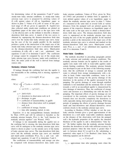
Selected Analytical Methods for Well and Aquifer Evaluation

for determining values of the parameters T and P´ understeady-state leaky artesian conditions. A steady-state leakyartesian type curve is prepared by plotting values ofK o (r/B) against values of r/B on logarithmic paper asshown in plate 2. Values of K o (r/B) in terms of the practicalrange of r/B are given in appendix B. Aquifer-testdata collected under steady-state conditions are plotted onlogarithmic paper of the same scale as the type curve withr as the abscissa and s as the ordinate to describe a distancedrawdownfield data curve. A match of the two curves isobtained by superposing the distance-drawdown field datacurve over the steady-state leaky artesian type curve, keepingthe axes of the two graphs parallel. In the matchedposition a point at the intersection of the major axes of thesteady-state leaky artesian type curve is selected and markedon the distance-drawdown field data curve. Match-pointcoordinates K o (r/B), r/B, s, and r are substituted intoequations 12 and 13 to determine T and P´. The coefficientof storage cannot be computed by use of the steady-stateleaky artesian type curve because, under such conditions offlow, the entire yield of the well is derived from leakagesources only.Nonleaky Artesian FormulaIf leakage through the confining bed into the aquifer isnot measurable or the confining bed is missing, equation 9becomess = (114.6Q/T) W (u) (14)where:andu =s=Q =T =r =2693r²S/Ttdrawdown in observation well, in ftdischarge, in gpmcoefficient of transmissibility, in gpd/ftdistance from observation well to pumpedwell, in ft(15)S = coefficient of storage, fractiont = time after pumping started, in minEquation 14 is the nonequilibrium formula introducedby Theis (1935) and will be referred to hereafter as thenonleaky artesian formula. W(u) is the “well function fornonleaky artesian aquifers” (see Wenzel, 1942).If leakage is not measurable during the aquifer test orthe confining bed is missing, the time-drawdown field datacurve will be analogous to the nonleaky artesian type curvewhich is shown in plate 1 as the outside curve of the familyof leaky artesian type curves. The time-drawdown field datacurve and the nonleaky artesian type curve are matched6and match point coordinates W(u), l/u, s, and t are substitutedinto equations 14 and 15 to determine T and S.The coefficients of transmissibility and storage can alsobe computed with distance-drawdown data under nonleakyartesian conditions. Values of W(u), given by Wenzel(1942) and presented in tabular form in appendix C,were plotted against values of u on logarithmic paper toobtain the nonleaky artesian type curve in plate 3. Valuesof s measured at the same time in several wells at variousdistances from the pumped well are plotted against thesquares of the respective distances on logarithmic paper ofthe same scale as the type curve to obtain a distance-drawdownfield data curve. The distance-drawdown field datacurve is superposed on the nonleaky artesian type curvekeeping the axes of the two graphs parallel. In the matchedposition a point at the intersection of the major axes of thenonleaky artesian type curve is selected and marked on thedistance-drawdown field data curve. Match-point coordinatesW(u), u, s, and r ² are substituted into equations 14and 15 to determine T and S.Water-Table ConditionsThe methods described in preceding paragraphs pertainto leaky artesian and nonleaky artesian conditions. Thenonleaky artesian formula can be applied to the results ofaquifer tests made with wells in water-table aquifers undercertain limiting conditions. The nonleaky artesian formulawas developed in part on the basis of the following assumptions:that the coefficient of storage is constant and thatwater is released from storage instantaneously with a declinein head. Under water-table conditions, water is derivedlargely from storage by the gravity drainage of theinterstices in the portion of the aquifer unwatered by thepumping. The gravity drainage of water through stratifiedsediments is not immediate and the nonsteady flow of watertowards a well in an unconfined aquifer is characterized byslow drainage of interstices. Thus, the coefficient of storagevaries and increases at a diminishing rate with the time ofpumping. The important effects of gravity drainage are notconsidered in the nonleaky artesian formula and thatformula does not describe completely the drawdown inwells especially during short periods of pumping. With longperiods of pumping the effects of gravity drainage becomesmall and time-drawdown and distance-drawdown curvesconform closely to the nonleaky artesian type curve.According to Boulton (1954a) whether or not the nonleakyartesian formula gives a good approximation of thedrawdown in a well under water-table conditions dependson the distance of the observation well from the pumpedwell r, the hydraulic properties of the aquifer, the saturatedthickness of the aquifer m, and a dimensionless “time factor.”He further implies that the nonleaky artesian formuladescribes the drawdown in wells with sufficient accuracy forpractical purposes when the time factor is greater than 5and r is between about 0.2 m and 6 m. By substituting anumerical value equal to 5 for Boulton’s time factor, thefollowing equation can be derived:t wt = 37.4S y m/P (16)where:t wt = approximate time after pumping starts when the