Selected Analytical Methods for Well and Aquifer Evaluation

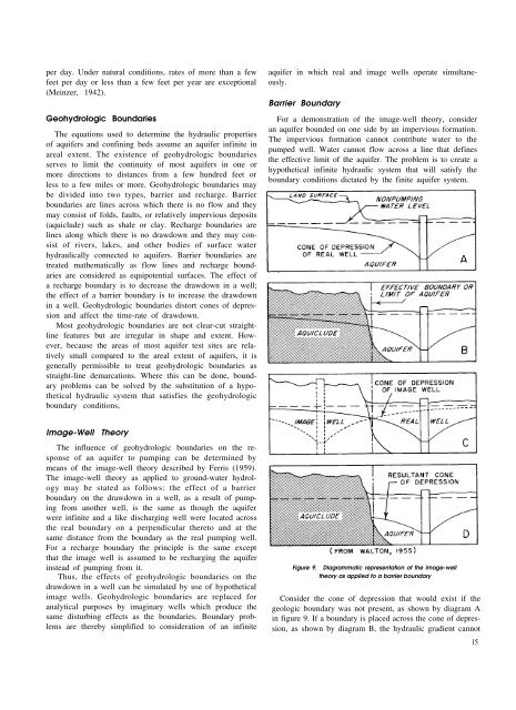
per day. Under natural conditions, rates of more than a fewfeet per day or less than a few feet per year are exceptional(Meinzer, 1942).Geohydrologic BoundariesThe equations used to determine the hydraulic propertiesof aquifers and confining beds assume an aquifer infinite inareal extent. The existence of geohydrologic boundariesserves to limit the continuity of most aquifers in one ormore directions to distances from a few hundred feet orless to a few miles or more. Geohydrologic boundaries maybe divided into two types, barrier and recharge. Barrierboundaries are lines across which there is no flow and theymay consist of folds, faults, or relatively impervious deposits(aquiclude) such as shale or clay. Recharge boundaries arelines along which there is no drawdown and they may consistof rivers, lakes, and other bodies of surface waterhydraulically connected to aquifers. Barrier boundaries aretreated mathematically as flow lines and recharge boundariesare considered as equipotential surfaces. The effect ofa recharge boundary is to decrease the drawdown in a well;the effect of a barrier boundary is to increase the drawdownin a well. Geohydrologic boundaries distort cones of depressionand affect the time-rate of drawdown.Most geohydrologic boundaries are not clear-cut straightlinefeatures but are irregular in shape and extent. However,because the areas of most aquifer test sites are relativelysmall compared to the areal extent of aquifers, it isgenerally permissible to treat geohydrologic boundaries asstraight-line demarcations. Where this can be done, boundaryproblems can be solved by the substitution of a hypotheticalhydraulic system that satisfies the geohydrologicboundary conditions,aquifer in which real and image wells operate simultaneously.Barrier BoundaryFor a demonstration of the image-well theory, consideran aquifer bounded on one side by an impervious formation.The impervious formation cannot contribute water to thepumped well. Water cannot flow across a line that definesthe effective limit of the aquifer. The problem is to create ahypothetical infinite hydraulic system that will satisfy theboundary conditions dictated by the finite aquifer system.Image-Well TheoryThe influence of geohydrologic boundaries on the responseof an aquifer to pumping can be determined bymeans of the image-well theory described by Ferris (1959).The image-well theory as applied to ground-water hydrologymay be stated as follows: the effect of a barrierboundary on the drawdown in a well, as a result of pumpingfrom another well, is the same as though the aquiferwere infinite and a like discharging well were located acrossthe real boundary on a perpendicular thereto and at thesame distance from the boundary as the real pumping well.For a recharge boundary the principle is the same exceptthat the image well is assumed to be recharging the aquiferinstead of pumping from it.Thus, the effects of geohydrologic boundaries on thedrawdown in a well can be simulated by use of hypotheticalimage wells. Geohydrologic boundaries are replaced foranalytical purposes by imaginary wells which produce thesame disturbing effects as the boundaries. Boundary problemsare thereby simplified to consideration of an infiniteFigure 9. Diagrammatic representation of the image-welltheory as applied to a barrier boundaryConsider the cone of depression that would exist if thegeologic boundary was not present, as shown by diagram Ain figure 9. If a boundary is placed across the cone of depression,as shown by diagram B, the hydraulic gradient cannot15