SSL II USER'S GUIDE - Lahey Computer Systems

SSL II USER’S GUIDE(Scientific Subroutine Library)

PREFACEThis manual describes the functions and use of the Scientific Subroutine Library II (SSL II),SSL II can be used for various systems ranging from personal computers to vector computers.The interface between a user-created program and SSL II is always the same regardless of thesystem type. Therefore, this manual can be used for all systems that use SSL II. When usingSSL II for the first time, the user should read “How to Use This Manual” first.The contents of SSL II or this manual may be amended to keep up with the latest state oftechnology, that is, if the revised or added subroutines should functionally include or surpasssome of the old subroutines, those old subroutines will be deleted in a time of allowance.Note:Some of the SSL II functions may be restricted in certain systems due to hardwarerestrictions. These functions are in the SSL II Subroutine List in this manual.

This document contains technology relating to strategic products controlled by export control laws ofthe producing and/or exporting countries. This document or a portion thereof should not beexported (or reexported) without authorization from the appropriate governmental authorities inaccordance with such laws.FUJITSU LIMITEDFirst Edition June 1989The contents of this manual may be revised without prior notice.All Rights Reserved, Copyright© FUJITSU LIMITED 1989No part of this manual may be reproduced in any from without permission

ACKNOWLEDGEMENTSWe believe that a scientific subroutine library can be one of convenient vehicles for thedissemination of the fruits of investigation made by experts concerned with numericalanalysis, furthermore, through the library a user can make use of these new fruits withoutever having to become familiar with the technical details.This led us to conclude that we had better request as many experts as possible toimplement their new methods, and then promote distribution of them to a wide community ofusers. As a result of our efforts to show our idea to many experts or authorities and todiscuss continuously with them, we could fortunately get a common consensus from them.We are pleased to enumerate below experts who have contributed to SSL II until now inacknowledgment of their efforts.ContributorsNameMasatsugu TanakaIchizo NinomiyaTatsuo ToriiTakemitsu HasegawaKazuo HatanoYasuyo HatanoToshio YoshidaKaoru ToneTakashi KobayashiToshio HosonoOrganizationFaculty of Engineering, YamanashiUniversity, JapanFaculty of Management InformationChubu University, JapanFaculty of Engineering, NagoyaUniversity, JapanFaculty of Engineering, FukuiUniversity, JapanFaculty of Engineering, Aichi TechnicalUniversity, JapanDepartment of Education, ChukyoUniversity, JapanFaculty of Management InformationChubu University, JapanGraduate School for Policy Science,Saitama University, JapanGraduate School for Policy Science,Saitama University, JapanCollege of Science and Technology,Nihon University, Japan(Nov., 1987)Also, our thanks are due to many universities and research institutes, especially thoseshown below, for helpful discussions and advises on our project, for providing informationon recent algorithms, numerical comparisons, and for suggesting several importantimprovements in this users’ guide.OrganizationsComputation Center, Hokkaido UniversityComputation Center, Nagoya UniversityComputation Center, Kyoto UniversityComputation Center, Kyusyu UniversityJapan Atomic Energy Research InstituteIt would be another pleasure that users would appreciate the efforts by contributors, and onthe occasions of publication of users’ own technical papers they would advertise on thepapers as possible the fact of having used SSL II.

SSL II SUBROUTINE LISTThe SSL II functions are listed below. Generally, a single-precision routine and adouble-precision routine are available for each function. The subroutine name column givesthe names of single-precision routines. Double-precision routine names start with a D,followed by the single-precision names. If the use of a function is restricted due tohardware restrictions, it is indicated in the remarks column.The symbols that appear in the remarks column mean the following:#: Only the single-precision routine is available in all systems.A. Linear AlgebraStorage mode conversion of matricesSubroutine name Item Page RemarksCGSM Storage mode conversion of matrices (real symmetric to real general) 264CSGM Storage mode conversion of matrices (real general to real symmetric) 290CGSBM Storage mode conversion of matrices (real general to real symmetric band) 263CSBGM Storage mode conversion of matrices (real symmetric band to real general) 287CSSBM Storage mode conversion of matrices (real symmetric to real symmetric band) 291CSBSM Storage mode conversion of matrices (real symmetric band to real symmetric) 289Matrix manipulationSubroutine name Item Page RemarksAGGM Addition of two matrices (real general + real general) 85SGGM Subtraction of two matrices (real general – real general ) 563MGGM Multiplication of two matrices (real general by real general) 454MGSM Multiplication of two matrices (real general by real symmetric) 465ASSM Addition of two matrices (real symmetric + real symmetric) 131SSSM Subtraction of two matrices (real symmetric – real symmetric) 582MSSM Multiplication of two matrices (real symmetric by real symmetric) 477MSGM Multiplication of two matrices (real symmetric by real general) 476MAV Multiplication of a real matrix by a real vector 456MCV Multiplication of a complex matrix by a complex vector 460MSV Multiplication of a real symmetric matrix by a real vector 478MSBV Multiplication of a real symmetric band matrix and a real vector 474MBV Multiplication of a real band matrix and a real vector 4581

Linear equationsSubroutine name Item Page RemarksLAX A system of linear equations with a real general matrix (Crout’s method) 388LCX A system of linear equations with a complex general matrix (Crout’s method) 407LSXLSIXLSBXLSBIXLBX1LSTXLTXLAXRLCXRLSXRLSIXRLSBXRLBX1RA system of linear equations with a positive-definite symmetric matrix (ModifiedCholesky’s method)A system of linear equations with a real indefinite symmetric matrix (Block diagonalpivoting method)A system of linear equations with a positive-definite symmetric band matrix(Modified Cholesky’s method)A system of linear equations with a real indefinite symmetric band matrix (blockdiagonal pivoting method)A system of linear equations with a real general band matrix (Gaussian eliminationmethod)A system of linear equations with a positive-definite symmetric tridiagonal matrix(Modified Cholesky’s method)A system of linear equations with a real tridiagonal matrix (Gaussian eliminationmethod)Iterative refinement of the solution to a system of linear equations with a realgeneral matrixIterative refinament of the solution to a system of linear equations with a complexgeneral matrixIterative refinement of the solution to a system of linear equations with apositive-definite symmetric matrixIterative refinament of the solution to a system of linear equations with a realindefinite symmetric matrixIterative refinament of the solution to a system of linear equations with apositive-definite symmetric band matrixIterative refinement of the solution to a system of linear equations with a realgeneral band matrix445438433431402442449399409447440435404Matrix inversionSubroutine name Item Page RemarksLUIV The inverse of a real general matrix decomposed into the factors L and U 452CLUIV The inverse of a complex general matrix decomposed into the factors L and U 279LDIVThe inverse of a positive-definite symmetric matrix decomposed into the factors L, D andL T 412Decomposition of matricesSubroutine name Item Page RemarksALU LU-decomposition of a real general matrix (Crout’s method) 98CLU LU-decomposition of a complex general matrix (Crout’s method) 277SLDLLDL T -decomposition of a positive-definite symmetric matrix (Modified Cholesky’s 570method)SMDMMDM T -decomposition of a real indefinite symmetric matrix (Block diagonal pivoting 572method)SBDLLDL T -decomposition of a positive-definite symmetric band matrix (Modified553Cholesky’s method)SBMDMMDM T -decomposition of a real indefinite symmetric band matrix (block diagonal 555pivoting method)BLU1 LU-decomposition of a real general band matrix (Gaussian elimination method) 1892

Solution of decomposed systemSubroutine name Item Page RemarksLUXCLUXLDLXMDMXBDLXBMDMXBLUX1A system of linear equations with a real general matrix decomposed into thefactors L and UA system of linear equations with a complex general matrix decomposed into thefactors L and UA system of linear equations with a positive-definite symmetric matrixdecomposed into the factors L, D and L T 414A system of linear equations with a real indefinite symmetric matrix decomposedinto the factors M, D and M T 462A system of linear equations with a positive-definite symmetric band matrixdecomposed into the factors L, D and L T 136A system of linear equations with a real indefinite symmetric band matrixdecomposed into factors M, D, and M T 192A system of linear equations with a real general band matrix decomposed into thefactors L and U454281186Least squares solutionSubroutine name Item Page RemarksLAXL Least squares solution with a real matrix (Householder transformation) 390LAXLR Iterative refinement of the least squares solution with a real matrix 397LAXLMLeast squares minimal norm solution with a real matrix (Singular value393decomposition method)GINV Generalized Inverse of a real matrix (Singular value decomposition method) 341ASVD1 Singular value decomposition of a real matrix (Householder and QR methods) 132B. Eigenvalues and EigenvectorsEigenvalues and eigenvectorsSubroutine name Item Page RemarksEIG1 Eigenvalues and corresponding eigenvectors of a real matrix (double QR method) 298CEIG2 Eigenvalues and corresponding eigenvectors of a complex matrix (QR method) 242SEIG1Eigenvalues and corresponding eigenvectors of a real symmetric matrix (QL 558method)SEIG2Selected eigenvalues and corresponding eigenvectors of a real symmetric matrix 560(Bisection method, inverse iteration method)HEIG2Eigenvalues and corresponding eigenvectors of an Hermition matrix (Householder 356method, bisection method, and inverse iteration method)BSEGEigenvalues and eigenvectors of a real symmetric band matrix206(Rutishauser-Schwarz method, bisection method and inverse iteration method)BSEGJ Eigenvalues and eigenvectors of a real symmetric band matrix (Jennings method) 208TEIG1Eigenvalues and corresponding eigenvectors of a real symmetric tridiagonal 583matrix (QL method)TEIG2Selected eigenvalues and corresponding eigenvectors of a real symmetric585tridiagonal matrix (Bisection method, inverse iteration method)GSEG2Eigenvalues and corresponding eigenvectors of a real symmetric generalized 347matrix system Ax = λ Bx (Bisection method, inverse iteration method)GBSEGEigenvalues and corresponding eigenvectors of a real symmetric band335generalized eigenproblem (Jennings method)3

EigenvaluesSubroutine name Item Page RemarksHSQR Eigenvalues of a real Hessenberg matrix (double QR method) 361CHSQR Eigenvalues of a complex Hessenberg matrix (QR method) 270TRQL Eigenvalues of a real symmetric tridiagonal matrix (QL method) 598BSCT1 Selected eigenvalues of a real symmetric tridiagonal matrix (Bisection method) 198EigenvectorsSubroutine name Item Page RemarksHVEC Eigenvectors of a real Hessenberg matrix (Inverse iteration method) 363CHVEC Eigenvectors of a complex Hessenberg matrix (Inverse iteration method) 272BSVEC Eigenvectors of a real symmetric band matrix (Inverse iteration method) 218OthersSubroutine name Item Page RemarksBLNC Balancing of a real matrix 184CBLNC Balancing of a complex matrix 239HES1 Reduction of a real matrix to a real Hessenberg matrix (Householder method) 358CHES2Reduction of a complex matrix to a complex Hessenberg matrix (Stabilized268elementary transformation)TRID1Reduction of a real symmetric matrix to a real symmetric tridiagonal matrix596(Householder method)TRIDHReduction of an Hermition matrix to a real symmetric tridiagonal matrix593(Householder method and diagonal unitary transformation)BTRIDReduction of a real symmetric band matrix to a tridiagonal matrix221(Rutishauser-Schwarz method)HBK1Back transformation and normalization of the eigenvectors of a real Hessenberg 354matrixCHBK2Back transformation of the eigenvectors of a complex Hessenberg matrix to the 266eigenvectors of a complex matrixTRBKBack transformation of the eigenvectors of a tridiagonal matrix to the eigenvectors 589of a real symmetric matrixTRBKHBack transformation of eigenvectors of a tridiagonal matrix to the eigenvectors of an 591Hermition matrixNRML Normalization of eigenvectors 498CNRML Normalization of eigenvectors of a complex matrix 283GSCHL Reduction of a real symmetric matrix system Ax = λ Bx to a standard form 345GSBKBack transformation of the eigenvectors of the standard form the eigenvectors of 343the real symmetric generalized matrix system4

C. Nonlinear EquationsSubroutine name Item Page RemarksRQDR Zeros of a quadratic with real coefficients 552CQDR Zeros of a quadratic with complex coefficients 286LOWP Zeros of a low degree polynomial with real coefficients (fifth degree or lower) 423RJETR Zeros of a polynomial with real coefficients (Jenkins-Traub method) 546CJART Zeros of a polynomial with complex coefficients (Jarratt method) 275TSD1Zero of a real function which changes sign in a given interval (derivative not604required)TSDM Zero of a real function (Muller’s method) 601CTSDM Zero of complex function (Muller’s method) 292NOLBR Solution of a system of nonlinear equations (Brent’s method) 487D. ExtremaSubroutine name Item Page RemarksLMINFMinimization of function with a variable (quadratic interpolation using function values 418only)LMINGMinimization of function with a variable (cubic interpolation using function values and 420its derivatives)MINF1Minimization of function with several variables (revised quasi-Newton method, uses 466function values only)MING1Minimization of a function with several variables (Quasi-Newton method, using 470function values and its derivatives)NOLF1Minimization of the sum of squares of functions with several variables (Revised 490Marquardt method, using function values only)NOLG1Minimization of the sum of squares of functions (revised Marquardt method using 494function values and its derivatives)LPRS1 Solution of a linear programming problem (Revised simplex method) 425NLPG1 Nonlinear programming (Powell’s method using function values and its derivatives) 482E. Interpolation and ApproximationInterpolationSubroutine name Item Page RemarksAKLAG Aitken-Lagrange interpolation 89AKHER Aitkan-Hermite interpolation 86SPLV Cubic spline interpolation 579BIF1 B-spline interpolation (I) 156BIF2 B-spline interpolation (II) 158BIF3 B-spline interpolation (III) 160BIF4 B-spline interpolation (IV) 162BIFD1 B-spline two-dimensional interpolation (I-I) 151BIFD3 B-spline two-dimensional interpolation (III-III) 154AKMID Two-dimensional quasi-Hermite Interpolation 91INSPL Cubic spline interpolation coefficient calculation 377AKMIN Quasi-Hermite interpolation coefficient calculation 95BIC1 B-spline interpolation coefficient calculation (I) 143BIC2 B-spline interpolation coefficient calculation (II) 145BIC3 B-spline interpolation coefficient calculation (III) 147BIC4 B-spline interpolation coefficient calculation (IV) 149BICD1 B-spline two-dimensional interpolation coefficient calculation (I-I) 138BICD3 B-spline two-dimensional interpolation coefficient calculation (III-III) 1415

ApproximationSubroutine name Item Page RemarksLESQ1 Polynomial least squares approximation 416SmoothingSubroutine name Item Page RemarksSMLE1 Data smoothing by local least squares polynomials (equally spaced data points) 575SMLE2 Data smoothing by local least squares polynomials (unequally spaced data points) 577BSF1 B-spline smoothing 216BSC1 B-spline smoothing coefficient calculation 201BSC2 B-spline smoothing coefficient calculation (variable knots) 203BSFD1 B-spline two-dimensional smoothing 214BSCD2 B-spline two-dimensional smoothing coefficient calculation (variable knots) 194SeriesSubroutine name Item Page RemarksFCOSFFourier Cosine series expansion of an even function (Function input, fast cosine 312transform)ECOSP Evaluation of a cosine series 296FSINF Fourier sine series expansion of an odd function (Function input, fast sine transform) 324ESINP Evaluation of a sine series 302FCHEB Chabyshev series expansion of a real function (Function input, fast cosine transform) 306ECHEB Evaluation of a Chebyshev series 294GCHEB Differentiation of a Chebyshev series 339ICHEB Indefinite integral of a Chebyshev series 3676

Numerical QuadratureSubroutine name Item Page RemarksSIMP1 Integration of a tabulated function by Simpson’s rule (equally spaced) 564TRAP Integration of a tabulated function by trapezoidal rule (unequally spaced) 588BIF1BIF2BIF3BIF4Intergration of a tabulated function by B-spline interpolation (unequally spaceddiscrete points, B-spline interpolation)156158160162BSF1Smoothing differentiation and integration of a tabulated function by B-spline least 216squares fit (fixed knots)BIFD1BIFD3Integration of a two-dimensional tabulated function (unequally spaced lattice points,B-spline two-dimensional interpolation)151154BSFD1 Two-dimensional integration of a tabulated function by B-spline interpolation 214SIMP2 Integration of a function by adaptive Simpson’s rule 565AQN9 Integration of a function by adaptive Newton-Cotes 9-point rule 126AQC8 Integration of a function by a modified Clenshaw-Curtis rule 100AQE Integration of a function by double exponential formula 106AQEH Integration of a function over the semi-infinite interval by double exponential formula 110AQEI Integration of a function over the infinite interval by double exponential formula 112AQMC8 Multiple integration of a function by a modified Clenshaw-Curtis integration rule 115AQME Multiple integration of a function by double exponential formula 121H. Differential equationsSubroutine name Item Page RemarksRKG A system of first order ordinary differential equations (Runge-Kutta method) 550HAMNG A system of first order ordinary differential equations (Hamming method) 350ODRK1 A system of first order ordinary differential equations (Runge-Kutta-Verner method) 518ODAM A system of first order ordinary differential equations (Adams method) 500ODGE A stiff system of first order ordinary differential equations (Gear’s method) 5098

I. Special FunctionsSubroutine name Item Page RemarksCELI1 Complete elliptic Integral of the first kind K(x) 244CELI2 Complete elliptic integral of the second kind E(x) 245EXPI Exponentia l integral Ei( x), Ei( x)304SINI Sine integral S i (x) 569COSI Cosine integral C i (x) 285SFRI Sine Fresnel integral S(x) 562CFRI Cosine Fresnel integral C(x) 246IGAM1 Incomplete Gamma function of the first kind γ (ν , x) 372IGAM2 Incomplete Gamma function of the second kind Γ (ν , x) 373IERF Inverse error function erf -1 (x) 369IERFC Inverse complimented error function erfc -1 (x) 370BJ0 Zero-order Bessel function of the first kind J 0(x) 173BJ1 First-order Bessel function of the first kind J 1(x) 175BY0 Zero-order Bessel function of the second kind Y 0(x) 228BY1 First-order Bessel function of the second kind Y 1(x) 230BI0 Modified Zero-order Bessel function of the first kind I 0(x) 167BI1 Modified First-order Bessel function of the first kind I 1(x) 168BK0 Modified Zero-order Bessel function of the second kind K 0(x) 182BK1 Modified First-order Bessel function of the second kind K 1(x) 183BJN Nth-order Bessel function of the first kind J n (x) 169BYN Nth-order Bessel function of the second kind Y n (x) 223BIN Modified Nth-order Bessel function of the first kind I n (x) 164BKN Modified Nth-order Bessel function of the second kind K n (x) 177CBIN Modified Nth-order Bessel function of the first kind I n (z) with complex variable 232CBKN Modified Nth-order Bessel function of the second kind K n (z) with complex variable 236CBJN Integer order Bessel function of the first kind with complex variable J n (z) 233CBYN Integer order Bessel function of the second kind with complex variable Y n (z) 241BJR Real-order Bessel function of the first kind J ν (x) 171BYR Real-order Bessel function of the second kind Y ν (x) 224BIR Modified real-order Bessel function of the first kind I ν (x) 166BKR Real order modified Bessel function of the second kind K ν (x) 178CBJR Real-order Bessel function of the first kind with a complex variable J ν (z) 234NDF Normal distribution function φ (x) 480NDFC Complementary normal distribution function ψ (x) 481INDF Inverse normal distribution function φ -1 (x) 375INDFC Inverse complementary normal distribution function ψ -1 (x) 3769

J. Pseudo Random NumbersSubroutine name Item Page RemarksRANU2 Uniform (0, 1) pseudo random numbers 533 #RANU3 Shuffled uniform (0, 1) pseudo random numbers 536 #RANN1 Fast normal pseudo random numbers 528 #RANN2 Normal pseudo random numbers 530 #RANE2 Exponential pseudo random numbers 527 #RANP2 Poisson pseudo random integers 531 #RANB2 Binominal pseudo random numbers 525 #RATF1 Frequency test for uniform (0, 1) pseudo random numbers 538 #RATR1 Run test of up-and-down for uniform (0, 1) pseudo random numbers 540 #10

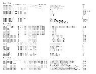
HOW TO USE THIS MANUALThis section describes the logical organization of thismanual, and the way in which the user can quickly andaccurately get informations necessary to him from themanual.This manual consists of two parts. Part I describes anoutline of SSL II. Part II describes usage of SSL IIsubroutines.Part I consists of twelve chapters.Chapter 2 describes the general rules which apply toeach SSL II subroutine. It is suggested that the userread this chapter first.Chapters 3 through 12 are concerned with certainfields of numerical computation, and were edited asindependently as possible for easy reference. At thebeginning of every chapter, the section “OUTLINE” isgiven, which describes the classification of availablesubroutines in the chapter, and how to select subroutinessuitable for a certain purpose. The user should read thesection at least once.As mentioned above, there is no confusing or difficultrelation between the chapters: it is quite simple as shownin the following diagram.Chapter 1Chapter 2Chapter 3Chapter 4Chapter 5Chapter 12Each chapter from chapter 3 on has several sections,the first of which is the section “OUTLINE” that, asnoted previously, introduces the following sections.As the diagram shows, if the user wants to obtaineigenvalues, for example, of a certain matrix, he shouldfirst read Chapter 2, then jump to Chapter 4, where hecan select subroutines suitable for his purposes.Part II describes how to use SSL II subroutines. Thesubroutines are listed in alphabetical order.When describing an individual subroutine, thefollowing contents associated with the subroutine areshown:• Function• Parameters• Comments on use• Methodand what we intend to describe under each title aboveare as follows:FunctionDescribes explanation of the functions.ParametersDescribes variables and arrays used for transmittinginformation into or from the subroutine. Generally,parameter names, which are commonly used in SSL II,are those habitually used so far in many libraries.Comments on useThis consists of the following three parts.• Subprograms usedIf other SSL II subroutines are used internally by thesubroutine, they are listed under “SSL II”. Also, ifFORTRAN intrinsic functions or basic externalfunctions are used, they are listed under “FORTRANbasic functions”.• NotesDiscusses various considerations that the user shouldbe aware of when using the subroutine.• ExampleAn example of the use of the subroutine is shown.For clarity and ease of understanding, any applicationsto a certain field of engineering or physical sciencehave not been described. In case other subroutinesmust be used as well as the subroutine to obtain amathematical solution, the example has been designedto show how other subroutines are involved. This isespecially true in the chapters concerning linearequations or eigenvalues etc. Conditions assumed inan example are mentioned at the beginning of theexample.MethodThe method used by the subroutine is outlined. Sincethis is a usage manual, only practical aspects of thealgorithm or computational procedures are described.References on which the implementation is based andthose which are important in theory, are listed inAppendix D “References”, so refer to them for furtherinformation or details beyond the scope of the “Method”section.In this manual, included are the SSL II Subroutine listand four appendices. In the SSL II Subroutine list, SSLII Subroutines are arranged in the order of fields and thenin the order of their classification codes. This list can beused for quick reference of subroutines.Appendix A explains the functions of the auxiliarysubroutines and Appendix B contains the three lists,which are concerned respectively with• General subroutines• Slave subroutines• Auxiliary subroutinesGeneral subroutines is an alphabetical listing of allsubroutines. In the list, if a certain entry uses othersubroutines, they are shown on the right. Slavesubroutines is an alphabetical listing of slave subroutines12

(as for the definition of them, see Section 2.1), and in thelist, general subroutines which use the slave subroutineare shown on the right. Auxiliary subroutines is a listingof auxiliary subroutines, and it is also alphabetical.Appendix C explains the subroutine names in order ofclassification code. This list can be used for quickreference of subroutines by classification code.Appendix D lists the documents referred for SSL IIdevelopment and/or logically important theory.Although no preliminary knowledge except the ability tounderstand FORTRAN is required to use this manual.Mathematical symbols used in this manual are listedbelow. We expect that the user has same interest in, orsome familiarity with numerical analysis.Mathematical symbol tableSymbol Example Meaning RemarksTA TTransposed matrix of matrix A⎡⎢⎢⎢⎣-1*⎤⎥⎥⎥⎦x TTransposed vector of column vector xx = (x 1 ,..., x n) T Column vector Refer to the symbol ( ).A -1Inverse of matrix AA *Conjugate transposed matrix of matrix Ax *Conjugate transposed vector of column vector xz * Conjugate complex number of complex number z z = a + ibz⎡⎢A = ⎢⎢⎣aaa1121n1aa1222aa1n⎤⎥⎥⎥⎦nnA is an n × n matrix whose elements are a ij.( ) x = (x 1 ,..., x n) T x is an n-dimensional column vector whose elements arex i.A = (a ij)Elements of matrix A are defined as a ij.x = (x i) Elements of column vector x are defined as x i.diag A = diag(a ii) Matrix A is a diagonal matrix whose elements are a ii.IUnit matrixdet det(A) Determinant of matrix Arank rank(A) Rank of matrix A|| || ||x|| Norm of vector xFor n-dimensional vector x , x = (x j) :A|| x |||| x ||n1 = ∑|x i |i = 1n22 = ∑|x i |i=1: Uniform norm: Euclidean norm|| x || = max|x i | : Infinity norm∞iRefer to symbols∑,, maxNorm of matrix AFor a matrix A = (a ij) of order n:⎛n⎞A = max⎜ ∑ a⎟∞ij: Infinity normij=1⎝ ⎠*z = a − ib( , ) (x, y) Inner product of vectors x and y When x and y are complex vectors,T( x,y)= x y(a, b)Open interval[ , ] [a, b] Closed interval>> a >> b a is much greater than b.≠ a ≠ b a is not equal to b.≈ f (x) ≈ P(x) f (x) is approximately equal to P(x).≡ f (x) ≡ f ′ (x) / f (x) f (x) is defined as f ′ (x) / f (x).{ } {x i} Sequence of numbers*z = z13

Symbol Example Meaning Remarksn∑Summation (x m ,..., x n)Sum cannot be given if n < m∑x ii=m∑ i + jix 2Summation with respect to iIfn∑ii=mi≠lx summation excludes x l.y′, f ′(x)dy df ( x)For n-order derivative:y′= , f ′(x)=dx dxf (n) nd f ( x)(x) =ndxz Absolute value of z If z = a + ibmax max(x 1 , ..., x n) The maximum value of (x 1, ..., x n)minsignmax xiimin(x 1 , ..., x n)min xiiThe minimum value of (x 1, ..., x n)sign(x)log log x Natural logarithm of xRe Re(z) Real part of complex number zIm Im(z) Imaginary part of complex number zarg Arg z Argument of complex number zδij2z = a + bSign of x When x is positive, 1.When x is negative, -1.Kronecker’s deltaγEuler’s constantπRatio of the circumference of the circle to its diameteri z = a + ib Imaginary unitP.V.P.V.a1b0+b∫ ∞ −x1ettdta2+ + ⋅⋅⋅b2Principal value of an integralContinued fraction∈ x ∈ X Element x is contained in set X.x x = ϕ(x)All elements of set x satisfy the equation.{ | } { }C k kf ( x)∈ C [ a,b]f (x) and up to k-th derivatives are continuous in theinterval [a , b].Note: This table defines how each symbol is used in this guide. A symbol may have a different meaning elsewhere. Commonly usedsymbols, such as + and – , were not included in the list.i =−1214

PART IGENERAL DESCRIPTION

CHAPTER 1SSL II OUTLINE1.1 BACKGROUND OF DEVELOPMENTMany years have passed since SSL (Scientific SubroutineLibrary) was first developed. Due to advancements innumerical calculation techniques and to increased powerof computers, SSL has been updated and new functionshave been added on many occasions. However, usershave further requested the followings:• Better balance of the functions and uses of individualsubroutines• That addition of new functions not adversely affect theorganization of the system• Better documentation of various functions and theirusesSSLII was developed with these requirements in mind.1.2 DEVELOPMENT OBJECTIVESSystematizingIt is important for a library to enable the user to quicklyidentify subroutines which will suit his purposes.SSLII is organized with emphasis on the followingpoints:• We classify numerical computations as follows:A Linear algebraB Eigenvalues and eigenvectorsC Nonlinear equationsD ExtremaE Interpolations and approximationsF TransformsG Numerical differentiation and quadratureH Differential equationsI Special functionsJ Pseudo random numbersThese categories are further subdivided for each branch.The library is made in a hierarchy organization. Theorganization allows easier identifying the locations ofindividual subroutines.• Some branches have subdivided functions. We presentnot only general purpose-oriented subroutines but alsothose which perform as components of the former, sothat the user can use the components when he wishes toanalize the sequence of the computational procedures.Performance improvementThrough algorithmic and programming revisions,improvements have been made both in accuracy andspeed.• The algorithmic methods which are stable and preciseare newly adopted. Some of the standard methods usedin the past are neglected.• In programming, importance is attached to reducingexecution time. Thus, the subroutines, are written inFORTRAN to enjoy the optimization of the compiler.SSLII improves the locality of the virtual storagesystem program, but does not decrease the efficiency ofa computer without virtual storage.Improvement of reliabilityIn most cases, single and double precision routines aregenerated from the same source program.Maintenance of compatibilityNowadays, developed softwares are easily transferredbetween different type systems. The SSL II subroutinesare structured to maintain compatibility. A few auxiliarysubroutines which are dependent of the system arecreated.1.3 FEATURES• SSL II is a collection of subroutines written inFORTRAN and desired subroutines are called in userprograms using the CALL statement.• All subroutines are written without input statements,user data is assumed to be in main storage.• Data size is defined with subroutine parameters. Norestrictions are applied to data size within subroutines.• To save storage space for linear and eigenvalue-17

GENERAL DESCRIPTIONeigenvector calculus, symmetric and band matrices arestored in a compressed mode (see Section 2.8 “DataStorage Methods”).• All subroutines have an output parameter whichindicates status after execution. A code giving the stateof the processing is returned with this parameter (referto Section 2.6 “Return Conditions of Processing”).Subroutines will always return control to the callingprogram. The user can check the contents of thisparameter to determine proper processing.• If specified, the condition messages are output (refer tosection 2.6 “return conditions of processing”).1.4 SYSTEM THAT CAN USE SSL IIIf the FORTRAN compilers can be used on the user’ssystem, SSL II can also be used regardless of the systemconfiguration. But, the storage size depends on thenumber and size of SSL II subroutines, the size of theuser program, and the size of the data.Although, as shown above, SSL II subroutines are usuallycalled by FORTRAN programs, they can also be calledby programs written in ALGOL, PL/1, COBOL, etc., ifthe system permits.When the user wishes to do that, refer to the section inFORTRAN (or another compiler) User’s Guide whichdescribes the interlanguage linkage.18

CHAPTER 2GENERAL RULES2.1 TYPES OF SUBROUTINESThere are three types of SSL II subroutines, as shown inTable 2.1.Table 2.1 Types of subroutinesSubroutinetypeGeneralsubroutineSlavesubroutineAuxiliarysubroutineSubprogramdivisionSubroutinesubprogramSubroutinesubprogramof functionsubprogramUseUsed by the user.Called by general subroutinesand cannot be called directlyby the user.Support general subroutinesand slave subroutines.The general subroutines in Table 2.1 are further divided,as shown in Table 2.2, into two levels according to thefunction. This division occurs when, in order to performsa particular function, a routine is internally subdividedinto elementary functions.Table 2.2 Subroutine levels2.3 SUBROUTINE NAMESEach of SSL II subroutines has the inherent subroutinename according to the subroutine type on followingconventions.General subroutine namesNames begin with S or D depending on the workingprecision, as shown in Fig. 2.2.Slave subroutine names• For subroutine subprograms or real functionsubprogramsNames begin with the working precision identifierwhich is same as in general subroutines followed by aletter ‘U’ as shown in Fig. 2.3.• For complex function subprogramsNames begin with letter ‘Z’. The other positions aresimilar to those shown above. See Fig. 2.4.Auxiliary subroutinesAuxiliary subroutines are appropriately named accordingto their functions, see Appendix A for details.LevelStandardroutineComponentroutineFunctionA single unified function is performed, forinstance, when solving a system of linearequations.An elementary function is performed, forinstance, for triangular factoring of a coefficientmatrix. Several component routines are groupedto make a standard routine.2.4 PARAMETERSTransmission of data between SSL II subroutines anduser programs is performed only through parameters.This section describes the types of SSL II parameters,their order, and precautions.2.2 CLASSIFICATION CODESEach of SSL II general subroutines has the elevencharacter classification codes according to theconventions in Fig. 2.1.Usage of parameters• Input/output parametersThese parameters are used for supplying values to thesubroutine on input, and the resultant values arereturned in the same areas on output.• Input parametersThese parameters are used for only supplying values tothe subroutine on input. The values are unchanged onoutput. If values are changed by subroutine, it isdescribed as “The contents of19

GENERAL DESCRIPTION1 2 3 4 5 6 7 8 9 10 113 digits: Subroutine numberSerial number assigned underthe same classification2 digits: Minor classification and appendingclassification1 digit: Middle classificationAlphabetic letter + 1 digit: Major classification1 digit: Subroutine level1…Standard routine2…Component routineABCDEFGHIJLinear algebraEigenvalues and eigenvectorsNon-linear equationsExtremaInterpolation and approximationTransformsNumerical differentiation and quadratureDifferential equationsSpecial functionsPseudo random numbersFig. 2.1 Classification code layoutparameter are altered on output” in parameter description.This alphanumeric string of up to 5 charactersidentifies the function of the subroutines.The last character, if numeric, groups subroutineswith related functions.1 alphabetic letter:This letter identifies the working precision.[S]…Single precision(normally S is omitted)D …Double precisionFig. 2.2 General subroutine namesUAn alphanumeric string of up to 4 characters:Corresponds to that of general subroutine.Fixed1 alphabetic letter:Identifies the working precision.Fig. 2.3 Subroutine names of slave subroutines (1)ZU• Output parametersThe resultant values are returned on output.• Work parametersThese are used as work areas. In general, the contentsof these parameters are meaningless on output.In addition, parameters can be also classified asfollows:• Main parametersThese parameters contain the data which is used as theobject of numerical calculations (for example, theelements of matrices).• Control parametersThese parameters contain data which is not used as theobject of numerical calculations (for example, the orderof matrices, decision values, etc.).Order of parameterGenerally, parameters are ordered according to their kindas shown in Fig. 2.5.An alphanumeric stringof up to 3 characters.Fixed1 alphabetic letter:Identifies the working precision.FixedFig. 2.4 Subroutine names of slave subroutines (2)20

GENERAL RULES( , , , , , , , ,ICON)EXTERNAL statement in the user program which callsthe SSL II subroutines.Output parametersInput parametersInput/output parametersWork parameters• Status after executionSSL II subroutines have a parameter named ICONwhich indicates the return conditions of processing.See Section 2.6.Note:The unshaded blocks indicate main parameters: the shadedblocks indicate control parameters. The ICON parameterindicates the return conditions of processing.Fig. 2.5 Parameter orderingSome control parameters cannot conform to Fig. 2.5 (forinstance, adjustable dimension of array), therefore theexplanation of each subroutine gives the actual ordering.Handling of parameters• Type of parameterType of parameter conforms to the ‘implicit typing’convention of FORTRAN except parameters that beginwith the letter ‘Z’. For instance, A is a 4 byte realnumber (8 byte real number in double precisionsubroutines) and IA is a standard-byte-length integer.When complex data is handled with complex variables,Z is the first letter of the parameter. ZA is an 8-bytecomplex number (16-byte complex number in doubleprecision subroutines).• External procedure nameWhen external procedure names are specified forparameters, those names must be declared with an2.5 DEFINITIONSMatrix classificationsMatrices handled by SSL II are classified as shown inTable 2.3.Table 2.3 Matrix classificationFactorsStructureFormTypeCharacterClassifications• Dense matrix• Band matrix• Symmetric matrix• Unsymmetric matrix• Real matrix• Complex matrix• Positive definite• Non singular• SingularPortion names of matrixIn SSL II, the portion names of matrix are defined asshown in Fig. 2.6. The portion names are usually usedfor collective reference of matrix elements.Where, the elements of the matrix are referred to as a ij .Upper triangular portion{Upper triangular elements |a ij ∈ A , j ≥ i+1}Lower triangular portion{Lower triangular elements | a ij ∈ A, i ≥ j+1}A=Second super-diagonal portion (*){Second super-diagonal elements | a ij ∈ A, j=i+2}(First) super-diagonal portion(*){(First) super-diagonal elements | a ij ∈ A, j=i+1}(Main) diagonal portion (*){(Main) diagonal elements | a ij ∈ A, i=j}(First)sub-diagonal portion{(First) sub-diagonal elements | a ij ∈ A, i=j+1}Second sub-diagonal portion(*){Second sub-diagonal elements | a ij ∈ A, i=j+2}Upper band portion{Upper band elements | a ij ∈ A, i+h 2 ≥ j ≥ i+1}Lower band portion{Upper band elements | a ij ∈ A, j+h 1 ≥ i ≥ j+1}(*) Sometimes called diagonal lineUpper band width h 2Lower band width h 1Fig. 2.6 Portion names of matrix21

GENERAL DESCRIPTIONMatrix definition and namingMatrices handled by SSL II have special namesdepending on their construction.• Upper triangular matrixThe upper triangular matrix is defined asa ij = 0 , j < i(2.1)Namely, the elements of the lower triangular portion arezero.• Unit upper triangular matrixThe unit upper triangular matrix is defined as⎧1,a ij = ⎨⎩0,j = ij < i(2.2)Namely, this matrix is the same as an upper triangularmatrix whose diagonal elements are all 1.• Lower triangular matrixThe lower triangular matrix is defined asa ij = 0 , j > i(2.3)Namely, the elements of the upper triangular portion arezero.• Unit lower triangular matrixThe unit lower triangular matrix is defined as⎧1,a ij = ⎨⎩0,j = ij > iThis matrix is the same as a lower triangular matrixwhose diagonal elements are all 1.• Diagonal matrixThe diagonal matrix is defined asa ij(2.4)= 0 , j ≠ i(2.5)Namely, all of the elements of the lower and the uppertriangular portions are zero.• Tridiagonal matrixThe tridiagonal matrix is defined as⎧0,j < i −1a ij = ⎨(2.6)⎩0,j > i + 1Namely, all of the elements except for ones of the upperand lower sub-diagonal and main-diagonal portions arezero.• Block diagonal matrixConsidering an n i × n j matrix A ij (i.e. a block) withinan n × n matrix A, where n=∑ ni=∑ nj, then the blockdiagonal matrix is defined asA = 0,i ≠ j(2.7)ijIn other words, all the blocks are on the diagonal line sothat the block diagonal matrix is represented by a directsum of those blocks.• Hessenberg matrixThe Hessenberg matrix is defined asa ij = 0,j < i −1(2.8)Namely, all of the elements except for ones of the uppertriangular, the main-diagonal and the lower sub-diagonalportions are zero.• Symmetric band matrixThe symmetric band matrix whose both upper andlower band widths are h is defined asaij⎪⎧0,= ⎨⎪⎩a ji ,i − j > hi − j ≤ hNamely, all of the elements except for ones of thediagonal, upper and lower band portions are zero.• Band matrixThe band matrix whose upper band width is h 1 , andlower band width is h 2 is defined as(2.9)⎧0,j > i + h2a ij = ⎨(2.10)⎩0,i > j + h1Namely, all of the elements except for ones of thediagonal, the upper and lower band portions are zero.• Upper band matrixThe upper band matrix whose upper band width is h isdefined as⎧0,a ij = ⎨⎩0,j > i + hj < iNamely, all of the elements except for ones of thediagonal and upper band portions are zero.(2.11)• Unit upper band matrixThe unit upper band matrix whose upper band width is his defined as22

GENERAL RULES⎧1,⎪a ij = ⎨0,⎪⎩0,j = ij > i + hj < i(2.12)This matrix is the same as an upper band matrix whosediagonal elements are all 1.• Lower band matrixThe lower band matrix whose lower band width is h isdefined as⎧0,a ij = ⎨⎩0,j < i − hj > iNamely, all of the elements except for ones of thediagonal and lower band portions are zero.(2.13)• Unit lower ban matrixThe unit lower band matrix whose lower band width ish is defined as⎧1,⎪a ij = ⎨0,⎪⎩0,j = ij < i − hj > i(2.14)Namely, this matrix is the same as a lower band matrixwhose diagonal elements are all 1.• Hermitian matrixThe hermitian matrix is defined as*a ji = a ij(2.15)Namely, this matrix equals its conjugate transposematrix.Table 2.4 Condition codesCode Meaning Integrity of theresult0 Processing has The resultsended normally. are correct.1 ~ Processing has9999 ended normally.Auxiliaryinformation wasgiven.10000~1999920000~29999Restrictions wereemployed duringexecution in orderto complete theprocessing.Processing wasaborted due toabnormalconditions whichhad occurredduring processing.30000 Processing wasaborted due toinvalid inputparameters.The resultsare correcton therestrictions.The resultsare notcorrect.StatusNormalCautionAbnormalComments about condition codes• Processing control by code testingThe condition code had better be tested in the user’sprogram immediately after the statement which callsthe SSL II subroutine. Then, the processing should becontrolled depending on whether the results are corrector not.:CALL LSX (A, N, B, EPSZ, ISW, ICON)IF (ICON. GE. 20000) STOP:• Output of condition messagesThe SSL II subroutines have a function to outputcondition messages. Normally, these messages are notoutput. When the user uses message output controlroutine MGSET (SSL II auxiliary subroutine) messagesare automatically output.2.6 RETURN CONDITIONS OF PRO-CESSINGThe SSL II subroutines have a parameter called ICONwhich indicates the conditions of processing. Thesubroutine returns control with a condition code set inICON. The values of the condition code should be testedbefore using the results.Condition codesThe code value is a positive integer values that rangesfrom 0 to 30000. The code values are classified asshown in Table 2.4.Each subroutine has appropriate codes that aredescribed in the condition code table given in the sectionwhere each subroutine description is.2.7 ARRAYSSL II uses arrays to process vectors or matrices. Thissection describes the arrays used as parameters and theirhandling.Adjustable arrays, whose sizes are declared in an arraydeclaration in the program, are used by SSL II. The usermay prepare arrays the size of which are determinedcorresponding to the size of the data processed in the userprogram.One-dimensional arraysWhen the user stores n (= N) - dimensional vector b( =(b 1 , ...., b n ) T ) in a one-dimensional array B of size N,23

GENERAL DESCRIPTIONas shown below, various ways are possible. In examplesbelow, an attention should be paid to the parameter Bused in calling the subroutine LAX, which solves systemsof linear equations (n ≤ 10 is assumed).• A general exampleThe following describes the case in which a constantvector b is stored in a one-dimensional array B of size10, as B(1) = b 1 , B(2) = b 2 , ...DIMENSION B(10):CALL LAX ( ... , N, B, ... ):• An application exampleThe following describes the case in which a constantvector b is stored in the I-th column of a twodimensionalarray C (10, 10), such that C (1, I) = b 1 , C(2, I) = b 2 , .....DIMENSION C(10, 10):CALL LAX ( ... , N, C(1, I), ... ):As shown in the above example, in parameter B, if aleading element (leading address) of one array in whichthe data is stored consecutively is specified it is notconstrained to a one-dimensional array of size N.Therefore, if vector b is stored in I-th row of array C asC(I, 1) = b 1 C (I, 2) = b 2 ... it is impossible to call asfollows.:CALL LAX ( ... , N, C(I, 1), ... ):Two-dimensional arraysConsider an n × n real matrix A (=(a ij )) being stored in atwo-dimensional array A (K, N). Note that in handlingtwo dimensional arrays in SSL II subroutines, adjustabledimension K is required as an input parameter in additionto the array A and the order N. The adjustable dimensionused by SSL II means the number of rows K of twodimensionalarray A declared in the user program. Anexample using a two-dimensional array along with anadjustable dimension K is shown next. The key points ofthe example are parameters A and K of the subroutineLAX. (Here n ≤ 10).The following describes the case in which coefficientmatrix is stored in a two-dimensional array A (10, 10) asshown in Fig. 2.7, as A (1, 1) = a 11 , A (2, 1) = a 21 , ...., A(1, 2) = a 12 ....DIMENSION A (10, 10):K = 10CALL LAX (A, K, N, ... ):In this case, regardless of the value of N, the adjustabledimension must be given as K = 10.N10AdjustabledimensionThe n × n coefficient matrix isstored in this region whichbecomes the object of theprocessing of the SSL IIsubroutine.This is declared in the userprogram as a two-dimensionalarray A (10,10).Fig. 2.7 Example of a two-dimensional adjustable arrayWhen equations of different order are to be solved, ifthe largest order is NMAX, then a two-dimensional arrayA (NMAX, NMAX) should be declared in the userprogram. That array can then be used to solve all of thesets of equations. In this case, the value of NMAX mustalways be specified as the adjustable dimension.2.8 DATA STORAGEThis section describes data storage modes for matrices orvectors.MatricesThe methods for storing matrices depend on structure andform of the matrices. All elements of unsymmetric densematrices, called general matrices, are stored in twodimensionalarrays. For all other matrices, onlynecessary elements can be stored in a one-dimensionalarray. The former storage method is called “generalmode,” the latter “compressed mode.” Detaileddefinition of storage modes are as follows.• General modeGeneral mode is shown in Fig. 2.8.• Compressed mode for symmetric matrixAs shown in Fig. 2.9, the elements of the diagonal andthe lower triangular portions of the symmetric densematrix A are stored row by row in the one-dimensionalarray A.• Compressed mode for Hermitian matrixThe elements of the diagonal and the lower triangularportions of the Hermitian matrix A are stored in a twodimensionalarray A as shown in Fig. 2.10.24

GENERAL RULESTwo-demensional array A(K,L)⎡a11 a12 a13 a14 a15⎤⎢a a a a a⎥⎢ 21 22 23 24 25⎥A = ⎢a a a a a ⎥31 32 33 34 35⎢⎥⎢a41 a42 a43 a44 a45⎥⎢⎣a a a a a ⎥51 52 53 54 55 ⎦a 11 a 12 a 13 a 14 a 15a 21 a 22 a 23 a 24 a 25a 31 a 32 a 33 a 34 a 35a 41 a 42 a 43 a 44 a 45a 51 a 52 a 53 a 54 a 555KNOTE: · Correspondence a ij → A (I,J)· K is the adjustable dimensionLFig. 2.8 Storage of unsymmetric dense matrices⎡ a11⎤⎢⎥⎢a21 + i⋅b21 a22⎥⎢⎥A = ⎢a31 + i⋅ b31 a32 + i⋅b32 a33⎥⎢⎥⎢a41 + i⋅ b41 a42 + i⋅ b42 a43 + i⋅b43 a44⎥⎢⎥⎣a51 + i⋅ b51 a52 + i⋅ b52 a53 + i⋅ b53 a54 + i⋅b54 a55⎦Two-demensional array A(K,L)a 11 b 21 b 31 b 41 b 51a 21 a 22 b 32 b 42 b 52a 31 a 32 a 33 b 43 b 53a 41 a 42 a 43 a 44 b 54a 51 a 52 a 53 a 54 a 555KNote: Correspondence a ij → A(I,J)(i ≥ j)b ij → A(J,I)(i > j)Fig. 2.10 Storage of Hermitian matricesL⎡a11⎢⎢a21 a22A = ⎢⎢a31 a32 a33⎢⎣a a a a41 42 43 44⎤⎥⎥⎥⎥⎥⎦Note : Correspondence( I −1)⎛ I ⎞a ij→ A⎜+ J ⎟⎝ 2 ⎠The value of NT isn( n + 1)NT =2Where n :order of matrixFig. 2.9 Storage of symmetric dense matricesOne-dimensinal array Aof size NTa 11a 21a 22a 31a 32a 33a 41a 42• Compressed mode for symmetric band matrixThe elements of the diagonal and the lower bandportions of a symmetric band matrix A are stored rowby row in a one-dimensional array A as shown in Fig.2.11.• Compressed mode for band matrixThe elements of the diagonal and the upper and lowerband portions of an unsymmetric band matrix A arestored row by row in a one-dimensional array A asshown in Fig. 2.12.a 43a 44NT⎡a11⎤⎢⎥⎢a21 a22⎥⎢⎥A = ⎢a31 a32 a33⎥⎢⎥⎢ a42 a43 a44⎥⎢⎥⎣ 0 a53 a54 a55⎦Note : CorrespondenceFor i ≤ h+ 1,For j > h + 1,The value of NT isNT = n( h + 1) − h ( h + 1)Where n = orderof matrixh = bandwidtha → Aa→( I ( I −1)2 + J )A( hI + J − h( h + 1)2)Fig. 2.11 Storage of symmetric band matricesVectorsVector is stored as shown in Fig. 2.13.ijij2One dimensionalarray A of size NTa 11a 21a 22a 31a 32a 33a 42a 43a 44a 53a 54a 55NT25

GENERAL DESCRIPTION⎡a11 a120 ⎤⎢a a a⎥⎢ 21 22 23 ⎥A = ⎢a a a a ⎥31 32 33 34⎢⎥⎢ a42 a43 a44 a45⎥⎢⎣ 0 a a a ⎥53 54 55⎦One dimensinal array A of size NTa 11a 12**a 21ha 22a 23h*a 31a 32a 33hNTNote:· NT =nhh =min(h 1+h 2+1,n)where h 2: Upper band widthh 1: Lower band widthn : Order of metrixa 34a 42a 43a 44a 45a 53h· * Indicates an arbitrary valuea 54ha 55*Fig. 2.12 Storage of unsymmetric band matrices⎡ x1⎤⎢ ⎥⎢x2⎥⎢x3⎥⎢ ⎥x = ⎢ ⎥⎢ ⎥⎢ ⎥⎢ ⎥⎢ ⎥⎣x n ⎦One dimensional array A of size nFig. 2.13 Storage of vectorsx 1x 2x 3x nCoefficients of polynomial equationsThe general form of polynomial equation is shown in(2.16)nn−1na 0 x + a1x+ .... + an−1x+ an= 0(2.16)Regarding the coefficients as the elements of a vector,the vector is stored as shown in Fig. 2.14.Coefficients of approximating polynomialsThe general form of approximating polynomial is shownin (2.17).⎡a0⎤⎢ ⎥⎢a1⎥⎢a2⎥⎢ ⎥a = ⎢ ⎥⎢ ⎥⎢ ⎥⎢ ⎥⎢ ⎥⎣a n ⎦One dimensional array A of size n+1a 0a 1a 2n + 1a nFig. 2.14 Storage of the coefficients of polynomial equations⎡c0⎤⎢ ⎥⎢c1⎥⎢c2⎥⎢ ⎥c = ⎢ ⎥⎢ ⎥⎢ ⎥⎢ ⎥⎢ ⎥⎣c n ⎦One dimensional array A of size n+1c 0c 1c 2n + 1c nFig. 2.15 Storage of the coefficients of approximating polynomials2n() x = c + c x + c x + .... c xP 0 1 2 +(2.17)nRegarding the coefficients as the elements of a vector,the vector is stored as shown in Fig. 2.15.n26

GENERAL RULES2.9 UNIT ROUND OFFSSL II subroutines frequently use the unit round off.The unit round off is a basic concept in error analysisfor floating point arithmetic.DefinitionThe unit round off of floating-point arithmetic aredefined as follows:u = M 1-L / 2, for (correctly) rounded arithmeticu = M 1-L , for chopped arithmetic,where M is the base for a floating-point number system,and L is the number of digits used to hold the mantissa.In SSL II, the unit round off is used for convergencecriterion or testing loss of significant figures.Error analysis for floating point arithmetic is covered inthe following references:[1] Yamashita, S.On the Error Estimation in Floating-pointArithmeticInformation Processing in Japan Vol. 15, PP.935-939, 1974[2] Wilkinson, J.H.Rounding Errors in Algebraic ProcessHer Britannic Majesty’s Stationery Office,London 19632.10 ACCUMULATION OF SUMSAccumulation of sums is often used in numericalcalculations. For instance, it occurs in solving a systemof linear equations as sum of products, and incalculations of various vector operations.On the theory of error analysis for floating pointarithmetic, in order to preserve the significant figuresduring the operation, it is important that accumulation ofsums must be computed as exactly as possible.As a rule, in SSL II the higher precision accumulation isused to reduce the effect of round off errors.2.11 Computer ConstantsThis manual uses symbols to express computer hardwareconstants. The symbols are defined as follows:• fl max : Positive maximum value for the floating-pointnumber system(See AFMAX in Appendix A.)• fl min : Positive minimum value for the floating-pointnumber system(See AFMIN in Appendix A.)• t max : Upper limit of an argument for a trigonometricfunction (sin and cos)Upper limit of argument ApplicationSingle 8.23 x 10 5 FACOM M seriesprecisionFACOM S seriesDouble 3.53 × 10 15 SX/G 100/200 seriesprecisionFM series27

CHAPTER 3LINEAR ALGEBRA3.1 OUTLINEOperations of linear algebra are classified as in Table 3.1depending on the structure of the coefficient matrix andrelated problems.Table 3.1 Classification of operation for linear equationsStructures Problem ItemConversion of matrix storage mode 3.2Dense Matrix manipulation 3.3matrix Systems of linear equationsMatrix inversion3.4Least squares solution 3.5Band Matrix manipulation 3.3matrix Systems of linearequationsDirect method 3.4This classification allows selecting the most suitablesolution method according to the structure and form ofthe matrices when solving system of linear equations.The method of storing band matrix elements in memoryis especially important. It is therefore important whenperforming linear equations to first determine thestructure of the matrices.3.2 MATRIX STORAGE MODECONVERSIONIn mode conversion the storage mode of a matrix isconverted as follows:Real symmetric matrixReal general matrixReal symmetric band matrixThe method to store the elements of a matrix dependson the structure and form of the matrix.For example, when storing the elements of a realsymmetric matrix, only elements on the diagonal andlower triangle portion are stored. (See Section 2.8).Therefore, to solve systems of linear equations, SSL IIprovides various subroutines to handle different matrices.The mode conversion is required when the subroutineassumes a particular storage mode. The mode conversionsubroutines shown in Table 3.2 are provided for thispurpose.3.3 MATRIX MANIPULATIONIn manipulating matrices, the following basicmanipulations are performed.Table 3.2 Mode conversion subroutinesAfterconversionBeforeconversionGeneral modeCompressed mode forsymmetric matricesCompressed mode forsymmetric band matricesGeneral modeCSGM(A11-10-201)CSBGM(A11-40-0201)Compressed modefor symmetricmatricesCGSM(A11-10-0101)CSBSM(A11-50-0201)Compressed modefor symmetricband matricesCGSBM(A11-40-0101)CSSBM(A11-50-0101)28

LINEAR ALGEBRATable 3.3 Subroutines for matrix manipulationB or x Real general Real symmetric VectorAmatrixmatrixReal general matrix Addition AGGM(A21-11-0101)Subtraction SGGM(A21-11-0301)Multiplication MGGM(A21-11-0301)MGSM(A21-11-0401)MAV(A21-13-0101)Complex general matrix Multiplication MCV(A21-15-0101)Real symmetric matrix Addition ASSM(A21-12-0101)SubtractionSSSM(A21-12-0201)Multiplication MSGM(A21-12-0401)MSSM(A21-12-0301)MSV(A21-14-0101)Real general band matrix Multiplication MBV(A51-11-0101)Real symmetric band matrix Multiplication MSBV(A51-14-0101)• Addition/Subtraction of two matrices• Multiplication of a matrix by a vector• Multiplication of two matrices ABA ± BAxSSL II provides the subroutines for matrix manipulation,as listed in Table 3.3.Comments on useThese subroutines for multiplication of matrix byvector are designed to obtain the residual vector as well,so that the subroutines can be used for iterative methodsfor linear equations.3.4 LINEAR EQUATIONS ANDMATRIX INVERSION (DIRECT METHOD)This section describes the subroutines that is used tosolve the following problems.• Solve systems of linear equationsAx = bA is an n × n matrix, x and b are n-dimensionalvectors.• Obtain the inverse of a matrix A.• Obtain the determinant of a matrix A.In order to solve the above problems, SSL II providesthe following basic subroutines ( here we call themcomponent subroutines) for each matrix structure.(a) Numeric decomposition of a coefficient matrix(b) Solving based on the decomposed coefficient matrix(c) Iterative refinement of the initial solution(d) Matrix inversion based on the decomposed matrixCombinations of the subroutines ensure that systems oflinear equations, inverse matrices, and the determinantscan be obtained.• Linear equationsThe solution of the equations can be obtained bycalling the component routines consecutively asfollows::CALL Component routine from (a)CALL Component routine from (b):• Matrix inversionThe inverse can be obtained by calling the abovecomponents routines serially as follows::CALL Component routine from (a)CALL Component routine from (b):The inverse of band matrices generally result in densematrices so that to obtain such the inverse is notbeneficial. That is why those component routines forthe inverse are not prepared in SSL II.29

GENERAL DESCRIPTION• DeterminantsThere is no component routine which computes thevalues of determinant. However, the values can beobtained from the elements resulting fromdecomposion (a).Though any problem can be solved by properlycombining these component routines, SSL II also hasroutines, called standard routines, in which componentroutines are called internally. It is recommended that theuser calls these standard routines.Table 3.4 lists the standard routines and componentroutines.Comments on uses• Iterative refinement of a solutionIn order to refine the accuracy of solution obtained bystandard routines, component routines (c) should besuccessively called regarding the solution as the initialapproximation. In addition, the component routine (c)serves to estimate the accuracy of the initialapproximation.• Matrix inversionUsually, it is not advisable to invert a matrix whensolving a system of linear equations.Ax = b (3.1)That is, in solving equations (3.1), the solution shouldnot be obtained by calculating the inverse A -1 and thenmultiplying b by A -1 from the left side as shown in (3.2).x = A -1 b (3.2)Instead, it is advisable to compute the LUdecompositionof A and then perform the operations(forward and backward substitutions) shown in (3.3).Ly = bUx = yHigher operating speed and accuracy can be attainedby using method (3.3). The approximate number ofmultiplications involved in the two methods (3.2) and(3.3) are compared in (3.4).For (3.2)For (3.3)3n + n3n / 32Therefore, matrix inversion should only be performedwhen absolutely necessary.(3.3)(3.4)• Equations with identical coefficient matricesWhen solving a number of systems of linear equationsas in (3.5) where the coefficient matrices are theidentical and the constant vectors are the different,Ax = bAx12= b:12Ax m = b m⎫⎪⎬⎪⎪⎭(3.5)it is not advisable to decompose the coefficient A foreach equation. After decomposing A when solving thefirst equation, only the forward and backwardsubstitution shown in (3.3) should be performed forsolving the other equations. In standard routines, aparameter ISW is provided for the user to controlwhether or not the equations is the first one to solve withthe coefficient matrix.Notes and internal processingWhen using subroutines, the following should be notedfrom the viewpoint of internal processing.• Crout’s method, modified Cholesky’s methodIn SSL II, the Crout’s method is used for decomposing ageneral matrix. Generally the Gaussian elimination andthe Crout’s method are known for decomposing (as in(3.6)) general matrices.A = LU (3.6)where: L is a lower triangular matrix and U is an uppertriangular matrix.The two methods require the different calculation order,that is, the former is that intermediate values arecalculated during decomposition and all elements areavailable only after decomposition. The latter is thateach element is available during decomposition.Numerically the latter involves inner products for twovecters, so if that calculations can be performedprecisely, the final decomposed matrices are moreaccurate than the former.Also, the data reference order in the Crout’s method ismore localized during the decomposition process than inthe Gaussian method. Therefore, in SSL II, the Crout’smethod is used, and the inner products are carried outminimizing the effect of rounding errors.On the other hand, the modified Cholesky method isused for positive-definite symmetric matrices, that is, thedecomposition shown in (3.7) is done.30

LINEAR ALGEBRATable 3.4 Standard and component routinesProblem BasicfunctionsTypesof matrixReal general matrixComplex generalmatrixReal symmetricmatrixReal positivedefinitesymmetricmatrixReal general bandmatrix⎡Real tridiagonal⎤⎣⎢ matrix ⎦⎥Real symmetricband matrixReal positivedefinitesymmetricband matrix⎡Positive - definite ⎤⎢symmetric⎥⎢⎣tridiagonal matrix⎥⎦Standard routinesSystems oflinear equationsLAX(A22-11-0101)LCX(A22-15-0101)LSIX(A22-21-0101)LSX(A22-51-0101)LBX1(A52-11-0101)⎡ LTX ⎤⎣⎢ (A52 - 11- 0501) ⎦⎥LSBIX(A52-21-0101)LSBX(A52-31-0101)LSTX(A52-31-0501)Component routines(a) (b) (c) (d)ALU(A22-11-0202)CLU(A22-15-0202)SMDM(A22-21-0202)SLDL(A22-51-0202)BLU1(A52-11-0202)SBMDM(A52-21-0202)SBDL(A52-31-0202)LUX(A22-11-0302)CLUX(A22-15-0302)MDMX(A22-21-0302)LDLX(A22-51-0302)BLUX1(A52-11-0302)BMDMX(A52-21-0302)BDLX(A52-31-0302)LAXR(A32-11-0401)LCXR(A22-15-0401)LSIXR(A22-21-0401)LSXR(A22-51-0401)LBX1R(A52-11-0401)LSBXR(A52-31-0401)LUIV(A22-11-0602)CLUIV(A22-15-0602)LDIV(A22-51-0702)A = LDL T (3.7)where: L is a lower triangular matrix and D is adiagonal matrix.Matrices are decomposed as shown in Table 3.5.Table 3.5 Decomposed matricesKinds of matricesGeneral matricesPositive-definitesymmetricmatricesContents of decomposed matricesPA = LUL: Lower triangular matrixU: Unit upper triangular matrixP is a permutation matrix.A = LDL TL: Unit lower triangular matrixD: Diagonal matrixTo minimize calculation, thediagonal matrix is given as D -1• Pivoting and scalingLet us take a look at decomposition of the nonsingularmatrix given by (3.6).A = ⎡ 00 . 10 .⎣ ⎢⎤20 . 00 .⎥⎦(3.8)In this state, LU decomposition is impossible. And alsoin the case of (3.9)A = ⎡ 00001 . 10 .⎣ ⎢⎤10 . 10 .⎥⎦(3.9)solutions. These unfavorable conditions can frequentlyoccur when the condition of a matrix is not proper. Thiscan be avoided by pivoting, which selects the elementwith the maximum absolute value for the pivot.In the case of (3.9), problems can be avoided byexchanging the first row with the second row.In order to perform pivoting, the method used to selectthe maximum absolute value must be unique. Bymultiplying all of the elements of a row by a large enoughconstant, any absolute value of non-zero element in therow can be made larger than those of elements in theother rows.Therefore, it is just as important to equilibrate the rowsand columns as it is to validly determine a pivot elementof the maximum size in pivoting. SSL II uses partialpivoting with row equilibration.The row equilibration is performed by scaling so thatthe maximum absolute value of each row of the matrixbecomes 1. However, actually the values of the elementsare not changed in scaling; the scaling factor is usedwhen selecting the pivot.Since row exchanges are performed in pivoting, thehistory data is stored as the transposition vector. Thematrix decomposition which accompanies this partialpivoting can be expressed as;PA = LU (3.10)Where P is the permutation matrix which performs rowexchanges.Decomposing by floating point arithmetic with the onlythree working digits (in decimal) will cause unstable31

GENERAL DESCRIPTION• Transposition vectorsAs mentioned above, row exchange with pivoting isindicated by the permutation matrix P of (3.10) in SSLII. This permutation matrix P is not stored directly, butis handled as a transposition vector. In other words, inthe j-th stage (j = 1, ... , n) of decomposition, if the i-throw (i ≥ j) is selected as the j-th pivotal row, the i-throw and the j-th row of the matrix in the decompositionprocess are exchanged and the j-th element of thetransposition vector is set to i.• How to test the zero or relatively zero pivotIn the decomposition process, if the zero or relativelyzero pivot is detected, the matrix can be considered tobe singular. In such a case, proceeding the calculationmight fail to obtain the accurate result. In SSL II,parameter EPSZ is used in such a case to determinewhether to continue or discontinue processing. In otherwords, when EPSZ is set to 10 -s and, if a loss of over ssignificant digits occurred, the pivot might beconsidered to be relatively zero.• Iterative refinement of a solutionTo solve a system of linear equations numericallymeans to obtain only an approximate solution to:Ax = b (3.11)SSL II provides a subroutine to refine the accuracy ofthe obtained approximate solution.SSL II repeats the following calculations until a certainconvergence criterion is satisfied.r( s)( s)= b − Ax(3.12)( s)( s)Ad = r(3.13)( s + 1) ( s)( s)x = x + d(3.14)where s = 1, 2, ... and x (1) the initial solution obtainedfrom (3.11).The x (2) could become the exact solution of (3.11) if allthe computations from (3.12) through (3.14) were carriedout exactly, as can be seen by the following.( )() ()( 2) () 1 () 1 1 1Ax A x d Ax r b= + = + =Actually, however, rounding errors will be generated inthe computation of Eqs. (3.12), (3.13) and (3.14).If we assume that rounding errors occur only when thecorrection d (s) is computed in Eq. (3.13), d (s) can beregarded to be the exact solution of the followingequation( s)( s)( A E) d = r+ (3.15)From Eqs. (3.12), (3.14) and (3.15), the followingrelationships can be obtained.−1s(1[ I − ( A + E)A] ( x − x)−1s(1)[ I − A( A + E)] r( s + 1))x − x =(3.16)r( s+1)= (3.17)As can be seen from Eqs. (3.16) and (3.17), if thefollowing conditions are satisfied, x (s+1) and r (s+1)converge to the solutions X and 0, respectively, as s→∞.I −−1−1( A + E) A , I − A( A + E) < 1∞In other words, if the following condition is satisfied, anrefined solution can be obtained.−1E ⋅ A < 1/ 2(3.18)∞∞This method described above is called the iterativerefinement of a solutionThe SSL II repeats the computation until when thesolution can be refined by no more than one binary digit.This method will not work if the matrix A conditions are−1poor. A may become large, so that no refined∞solution will be obtained.• Accuracy estimation for approximate solutionSuppose e (1) (= x (1) – x) is an error generated when theapproximate solution x (1) is computed to solve a linearequations. The relative error is represented by(1) (1)e / x .∞ ∞From the relationship between d (1) and e (1) , and (3.12),(3.15), we obtain Eq.(3.19).d(1)−1(1)−1−1(1)( A + E) ( b − Ax ) = ( I + A E) e= (3.19)If the iterative method satisfies the condition (3.18) and(1)converges, d is assumed to be almost equal to(1)e∞∞. Consequently, a relative error for anapproximate solution can be estimated by∞(1)∞d /3.5 LEAST SQUARES SOLUTION(1)x .∞Here, the following problems are handled:• Least squares solution• Least squares minimal norm solution• Generalized inverse• Singular value decompositionSSL II provides the subroutines for the above functionsas listed in Table 3.6.where E is an error matrix.32

LINEAR ALGEBRATable 3.6 Subroutines for m × n matricesKinds of matrixFunctionLeast squares solutionIterative refinement of theleast squares solutionLeast squares minimalnorm solutionGeneralized inverseSingular valuedecompositionReal matrixLAXL(A25-11-0101)LAXLR(A25-11-0401)LAXLM(A25-21-0101)GINV(A25-31-0101)ASVD1(A25-31-0201)• Least squares solutionThe least squares solution means the solution x ~ whichminimizes Ax − b , where A is an m × n matrix (m ≥2n, rank (A) = n), x is an n-dimensional vector and b isan m-dimensional vector.SSL II has two subroutines which perform thefollowing functions.− Obtaining the least squares solution− Iterative refinement of the least squares solution• Least squares minimal norm solutionThe least squares minimal norm solution means thesolution x + which minimizes x within the set of x2where Ax − b has been minimized, where A is an m2× n matrix, x is an n-dimensional vector and b is an m-dimensional vector.• Generalized inverseWhen n × m matrix X satisfies the following equationsin (3.20) for a given m × n matrix A, it is called aMoor-Penrose generalized inverse of the matrix A.AXA = A ⎫XAX = X⎪⎪T ⎬(3.20)( AX ) = AX( )⎪ ⎪ TXA = XA ⎭The generalized inverse always exists uniquely. Thegeneralized inverse X of a matrix A is denoted by A +SSL II calculates the generalized inverse as above.SSL II can handle any m × n matrices where:− m is larger than n− m is equal to n− m is smaller than n• Singular value decompositionSingular value decomposition is obtained bydecomposing a real matrix A of m × n as shown in(3.21).A = U 0 Σ 0 V T (3.21)Here U 0 and V are orthogonal matrices of m × m and n ×n respectively, Σ 0 is an m × n diagonal matrix whereΣ 0=diag(σ i) and σ i ≥ 0. The σ i are called singularvalues of a real matrix A. Suppose m ≥ n in real matrix Awith matrix m × n. Since Σ 0 is an m × n diagonal matrix,the first n columns of U 0 are used for U 0 Σ 0V T in (3.21).That is, U 0 may be considered as an n × n matrix. Let Ube this matrix, and let Σ be an n × n matrix consisting ofmatrix Σ 0 without the zero part, (m-n) × n, of Σ 0. Whenusing matrices U and Σ , if m is far larger than n, thestorage space can be reduced. So matrices U and Σ aremore convenient than U 0 and Σ 0 in practice. The samediscussion holds when m < n, in which case only the firstm raws of V T are used and therefore V T can beconsidered as m × n matrix.Considering above ideas SSL II performs the followingsingular value decomposition.A = UΣ V T (3.22)where: l = min (m, n) is assumed and U is an m × l matrix,Σ is an l × l diagonal matrix whereΣ = diag (σ i), and σ i ≥ 0, and V is an n × l matrix.When l = n (m ≥ n),TTU U = V V = VV =when l = m ( m < n ),TU U = UU = V V =TTTI nI mMatrices U, V and Σ which are obtained by computingsingular values of matrix A are used and described asfollows;(For details, refer to reference [86],)– Singular values σ i, i = 1, 2, ... , l are the positivesquare roots of the largest l eigenvalues of matrices A T Aand AA T . The i-th column of matrix V is the eigenvectorof matrix A T A corresponding to eigenvalue σ i 2 . The i-thcolumn of matrix U is the eigenvector of matrix AA Tcorresponding to eigenvalue σ i 2 . This can be seen bymultiplying A T = VΣ U T from the right and left sides of(3.22) and apply U T U = V T V = I l as follows:A T AV = VΣ 2 (3.23)AA T U = UΣ 2 (3.24)– Condition number of matrix AIf σ i > 0, i = 1, 2, ..., l, then condition number of matrixA is given as follows;cond(A) = σ 1 / σ l (3.25)– Rank of matrix AIf σ r > 0, and σ r+1 = ... = σ l = 0, then the rank of A isgiven as follows:33

GENERAL DESCRIPTIONrank (A) = r (3.26)– Basic solution of homogeneous linear equations Ax = 0and A T y = 0The set of non-trivial linearly independent solutions ofAx = 0 and A T y = 0 is the set of those columns ofmatrices V and U, respectively, corresponding tosingular values σ i = 0. This can be easily seen fromequations AV = UΣ and A T U = VΣ .– Least squares minimal norm solution of Ax = b.The solution x is represented by using singular valuedecomposition of A ;x = VΣ + U T b (3.27)where diagonal matrix Σ + is defined as follows:++++Σ = diag( σ1, σ2,..., σl )(3.28)σ + ⎧1/σi, σi> 0i = ⎨⎩0, σi= 0(3.29)For details, refer to “Method” of subroutine LAXLM.– Generalized inverse of a matrixGeneralized inverse A + of A is given after decomposingA into singular value as follows;A + = VΣ + U T (3.30)Comments on uses– Systems of linear equations and the rank of coefficientmatricesSolving the systems of linear equations (Ax = b) withan m × n matrix as coefficient, the least squaresminimal norm solution can be obtained regardless ofthe number of columns or rows, or ranks of coefficientmatrix A. That is, the least squares minimal normsolution can be applied to any type of equations.However, this solution requires a great amount ofcalculation for each process. If the coefficient matrix isrectangular and number of rows is larger than that ofcolumns and the rank is full (full rank, rank(A) = n),you should use the subroutine for least squares solutionbecause of less calculation. In this case, the leastsquares solution is logically as least squares minimalnorm solution.• Least squares minimal norm solution and generalizedinverseThe solution of linear equations Ax = b with m × nmatrix A (m ≥ n or m < n, rank(A) ≠ 0) is not uniquelyobtained. However, the least squares minimal normsolution always exists uniquely.This solution can be calculated by x = A + b aftergeneralized inverse A + of coefficient matrix A isobtained. This requires a great amount of calculation.It is advisable to use the subroutine for the leastsquares minimal norm solution, for the sake of highspeed processing. This subroutine provides parameterISW by which the user can specify to solve theequations with the same coefficient matrix with lesscalculation or to solve the single equation withefficiency.• Equations with the identical coefficient matrixThe least squares solution or least squares minimalnorm solution of a system of linear equations can beobtained in the following procedures;− Decomposition of coefficient matricesFor the least squares solution a matrix A isdecomposed into triangular matrices , and for theleast squares minimal norm solution A isdecomposed into singular values− Obtaining solutionBackward substitution and multiplication of matricesor vectors are performed for the least-squaressolution and the least squares minimal norm solution,respectively.When obtaining the least squares solution or leastsquares minimal norm solution of a number of systemswith the identical coefficient matrices, it is not advisableto repeat the decomposition for each system.AxAx12= b= b:12Ax m = b mIn this case, the matrix needs to be decomposed onlyonce for the first equations, and the decomposed formcan be used for subsequent systems , thereby reducing theamount of calculation.SSL II provides parameter ISW which can controlswhether matrix A is decomposed or not.• Obtaining singular valuesThe singular value will be obtained by singular valuedecomposition as shown in (3.31):A = UΣ V T (3.31)As shown in (3.31), matrices U and V are involvedalong with matrix Σ which consists of singular values.Since singular value decomposition requires a greatamount of calculation, the user need not to calculate Uand V when they are no use. SSL II provides parameterISW to control whether matrices U or V should beobtained. SSL II can handle any type of m × n matrices(m > n, m = n, m < n).34

CHAPTER 4EIGENVALUES AND EIGENVECTORS4.1 OUTLINEEigenvalue problems can be organized as show in Table4.1 according to the type of problem (Ax =λx, Ax =λBx)and the shape (dense, band), type (real, complex), andform (symmetric, unsymmetric) of the matrices. Thereader should refer to the appropriate section specifiedin the table.Table 4.1 Organization of eigenvalue problemShape ofmatrixDensematrixBandmatrixType ofproblemAx =λxMatrix type and formReal matrixComplex matrixReal symmetric matrixHermitian matrixExplanationsection4.24.34.44.5Ax =λBx Real symmetric matrix 4.7Ax =λx Real symmetric band 4.6matrixAx =λBx Real symmetric band 4.8matrixNote:Refer to the section on a real symmetric matrix concerning areal symmetric tridiagonal matrix.4.2 EIGENVALUES ANDEIGENVECTORS OF A REAL MATRIXA standard sequenses of procedures are shown herewhen SSL II routines are used to solve the eigenvalueproblems.SSL II provides the following:− Standard routines by which the entire procedures forobtaining eigenvalues and eigenvectors of realmatrices may be performed at one time.− Component routines performing component functions.For details, see Table 4.2.User problems are classified as follows :• Obtaining all eigenvalues• Obtaining all eigenvalues and correspondingeigenvectors (or selected eigenvectors)In the first and second items that follow, the use ofcomponent routines and standard routines is explainedby describing their procedures. Further comments onprocessing are in the third item.When obtaining eigenvalues and eigenvectors of a realmatrix, the choice of calling the various componentroutines or calling the standard routine is up to the user.However, the standard routine, which is easier to use, isrecommended to be called.Table 4.2 Subroutines used for standard eigenproblem of a real matrixLevel Function Subroutine nameStandard routines Eigenvalues and eigenvectors of a real matrixEIG1(B21-11-0101)Balancing of a real matrixBLNC(B21-11-0202)Reduction of a real matrix to a Hessenberg matrixHES1(B21-11-0302)HSQR(B21-11-0402)ComponentroutinesObtaining the eigenvalues of a real HessenbergmatrixObtaining the eigenvectors of a real HessenbergmatrixBack transformation to and normalization of theeigenvectors of a real matrixNormalization of the eigenvectors of a real matrixHVEC(B21-11-0502)HBK1(B21-11-0602)NRML(B21-11-0702)35

GENERAL DESCRIPTIONIn addition, obtaining the eigenvectors corresponding tospecified eigenvalues can only be done by calling a seriesof component routines.Obtaining all eigenvaluesIn the following programs, all eigenvalues of the realmatrix A are obtained through the use of the componentroutines shown in steps 1), 2), 3).:CALL BLNC (A, K, N, DV, ICON) 1)IF (ICON .EQ. 30000) GO TO 1000CALL HES1 (A, K, N, PV, ICON) 2)CALL HSQR (A, K, N, ER, EI, M,ICON)3)IF (ICON .EQ. 20000) GO TO 2000:1) A is balanced, if balancing is not necessary, this stepis omitted.2) Using the Householder method, A is reduced to aHessenberg matrix.3) By calculating the eigenvalues of the Hessenbergmatrix using the double QR method, the eigenvaluesof A are obtained.Obtaining all eigenvalues and correspondingeigenvectors (or selected eigenvectors)All eigenvalues and corresponding eigenvectors of realmatrix A can be obtained by calling the componentroutines shown in 1) to 5) or by calling the standardroutine shown in 6).:CALL BLNC (A, K, N, DV, ICON) 1)IF (ICON .EQ. 30000) GO TO 1000CALL HES1 (A, K, N, PV, ICON) 2)DO 10 I = 1, NDO 10 J = 1, NAW (J, I) = A (J, I)10 CONTINUECALL HSQR (A, K, N, ER, EI, M,ICON)3)IF (ICON .GE. 20000) GO TO 2000DO 20 I = 1, MIND (I) = 120 CONTINUECALL HVEC (AW, K, N, ER, EI, IND,*M, EV, MK, VW, ICON) 4)IF (ICON .GE. 20000) GO TO 3000CALL HBK1 (EV, K, N, IND, M, A, PV,* DV, ICON) 5):or standard routine.:CALL EIG1 (A, K, N, MODE, ER, EI, EV, VW, ICON) 6)IF(ICON .GE. 20000) GO TO 1000:1), 2), and 3) were explained in the preceding example“Obtaining all eigenvalues”. However since 3)destroys parameter A, A must be stored in array AWafter 2) so that contents of A before 3) can be used in4).4) The eigenvectors corresponding to the eigenvaluesare obtained using the inverse iteration method. Theparameter IND is an index vector which indicates theeigenvalues from which eigenvectors are to beobtained. The user can select eigenvectors using thisparameter.5) Back transformation of the eigenvectors obtained in4) is performed. The transformed eigenvectors arenormalized at the same time.From the processing of 1) and 2), the eigenvectors of4) are not the eigenvectors of real matrix A. Theeigenvectors of A are obtained by performing thepost-processing corresponding to 1) and 2).Each column (i.e., each eigenvector) of parameterEV is normalized such that its Euclidean norm is 1.6) When obtaining all eigenvalues and correspondingeigenvectors of a real matrix, the functions of 1) to 5)can be performed by calling this standard routine,however, instead of using the inverse iteration method,all eigenvectors are obtained at a time by multiplyingall the transformation matrices obtained successively.This calculation will not work if even one eigenvalueis missing.However, if eigenvalues are close roots or multipleroots, eigenvectors can be determined moreaccurately using this method than the inverse iterationmethod. The standard routine 6) does not alwaysperform the process in step 1). The parameter MODEcan be used to specify whether step 1) is performed ornot.Balancing of matricesErrors on calculating eigenvalues and eigenvectors can bereduced by reducing the norm of real matrix A. Routine1) is used for this purpose. By diagonal similaritytransformation the absolute sum of row i and that ofcolumn i in A is made equal (this is called balancing).Symmetric matrices and Hermitian matrices are alreadybalanced. Since this method is especially effective whenmagnitudes of elements in A differ greatly, balancingshould be done. Except in certain cases (i.e. when thenumber of the order of A is small), balancing should nottake more than 10% of the total processing time.4.3 EIGENVALUES ANDEIGENVECTORS OF A COMPLEXMATRIXAn example will be used to show how the various SSL IIsubroutines obtain eigenvalues and eigenvectors of acomplex matrix.36

EIGENVALUES AND EIGENVECTORSTable 4.3 Subroutines used for standard eigenproblem of a complex matrixLevel Function Subroutine nameStandard routine Eigenvalues and eigenvectors of a complex matrixCEIG2(B21-15-0101)Balancing of a complex matrixCBLNC(B21-15-0202)Reduction of a complex matrix to a complexHessenberg matrixCHES2(B21-15-0302)ComponentObtaining the eigenvalues of a complex HessenbergmatrixCHSQR(B21-15-0402)routineObtaining the eigenvectors of a complex HessenbergmatrixCHVEC(B21-15-0502)Back transformation to the eigenvectors of a complexmatrixCHBK2(B21-15-0602)Normalization of the eigenvectors of a complex matrixCNRML(B21-15-0702)SSL II provides the following:− Standard routines by which the entire procedures forobtaining eigenvalues and eigenvectors of complexmatrices may be performed at one time.− Component routines performing component functionsFor details, see Table 4.3User problems are classified as follows:• Obtaining all eigenvalues• Obtaining all eigenvalues and correspondingeigenvectors (or selected eigenvectors)In the first and second items that follow, the use ofcomponent routines and standard routines are explainedby describing their procedures.When obtaining all eigenvalues and correspondingeigenvectors whether the standard routines only or thevarious corresponding component routines are used is upto the user. However it is recommended to call theformer for its easy handling.Obtaining all eigenvaluesIn the following programs, all eigenvalues of the complexmatrix A are obtained through the use of the componentroutines shown in steps 1), 2), and 3).CALL CBLNC (ZA, K, N, DV, ICON) 1)IF (ICON. EQ. 30000) GO TO 1000CALL CHES2 (ZA, K, N, IP, ICON) 2)CALL CHSQR (ZA, K, N, ZE, M, ICON) 3)IF (ICON. GE. 15000) GO TO 20001) A is balanced. If balancing is not necessary, this stepis omitted.2) Using the stabilized elementary transformation, A isreduced to a complex Hessenberg matrix.3) By calculating the eigenvalues of the complexHessenberg matrix using the complex QR method, theeigenvalues of A are obtained.Obtaining all eigenvalues and the correspondingeigenvectors (or selected eigenvectors)All eigenvalues and the corresponding eigenvectors of acomplex matrix A can be obtained by calling thecomponent routines shown in 1) to 6) or by calling thestandard routine shown in 7).:CALL CBLNC (ZA, K, N, DV, ICON) 1)IF (ICON. EQ. 30000) GO TO 1000CALL CHES2 (ZA, K, N, IP, ICON) 2)DO 10 J = 1, NDO 10 I = 1, NZAW (I, J) = ZA (I, J)10 CONTINUECALL CHSQR (ZA, K, N, ZE, M, ICON) 3)IF (ICON. GE. 15000) GO TO 2000DO 20 I = 1, MIND (I) = 120 CONTINUECALL CHVEC (ZAW, K, N, ZE, IND,* M, ZEV, ZW, ICON) 4)IF (ICON. GE. 15000) GO TO 3000CALL CHBK2 (ZEV, K, N, IND, M, ZP,* IP, DV, ICON) 5)CALL CNRML (ZEV, K, N, IND, M, 1,* ICON) 6)or standard routine:CALL CEIG2 (ZA, K, N, MODE, ZE,*ZEV, VW, IVW, ICON) 7)IF (ICON. GE. 20000) GO TO 1000:1), 2), and 3) were explained in the preceding example“Obtaining all eigenvalues”. However since 3)destroys parameter ZA, ZA must be stored in arrayZAW after 2) so that contents of ZA before 3) can beused in 4) and the subsequent routines.4) The eigenvectors of the complex Hessenberg matrixcorresponding to the eigenvalues are obtained usingthe inverse iteration method. The parameter IND isan index vector which indicates the eigenvalues fromwhich eigenvectors are to be obtained. The user canselect eigenvectors using this parameter.5) Back transformation of the eigenvectors obtained in4) is performed to obtain the eigenvectors of A.6) The eigenvectors transformed in 5) are normalized.When normalizing the eigenvectors (set norm to 1),the user can select whether an Euclidean or infinitynorm should be used. Here the former is applied fornormalization.7) When obtaining all eigenvalues and correspondingeigenvectors of a complex matrix, the functions of 1)through 6) can be performed by calling this standard37

GENERAL DESCRIPTIONroutine, however, instead of using the inverse iterationmethod, all eigenvectors are obtained at one time bymultiplying all the obtained transformation matrices.This calculation will not work if even one of theeigenvalues is missing. The parameter MODE can beused to specify whether the matrix is to be balancedor not.4.4 EIGENVALUES ANDEIGENVECTORS OF A REALSYMMETRIC MATRIXAn example will be used here to show how the variousSSL II subroutines are used to obtain eigenvalues andeigenvectors of a real symmetric matrix.SSL II provides the followings:− Standard routines by which the entire procedures forobtaining eigenvalues and eigenvectors of a realsymmetric matrix may be performed at one time.− Component routines decomposed by functions.For details, see Table 4.4.The problems can be classified as follows:• Obtaining all eigenvalues.• Obtaining selected eigenvalues.• Obtaining all eigenvalues and correspondingeigenvectors.• Obtaining selected eigenvalues and correspondingeigenvectors.In the above order, the first four items below explain theuse of component routines and standard routines. Thelast two items provide additional information.The choice of calling individual component routines orof calling a single standard routine for obtaining alleigenvalues and corresponding eigenvectors or selectedeigenvalues and corresponding eigenvectors is up to theuser. Normally, standard routines which are easier to use,are selected. Component routines TEIG1 or TEIG2should be used if the real symmetric matrix is originallytridiagonal.SSL II handles the real symmetric matrix in symmetricmatrix compressed mode (For details, refer to Section2.8).Obtaining all eigenvaluesAll eigenvalues of a real symmetric matrix A can beobtained as shown below 1) and 2). A is handled in thecompressed storage mode, i.e., as a one-dimensionalarray, for a real symmetric matrix.:CALL TRID1 (A, N, D, SD, ICON) 1)IF (ICON .EQ. 30000) GO TO 1000CALL TRQL (D, SD, N, E, M, ICON) 2):Table 4.4 Subroutines used for standard eigenproblem of a real symmetric matrix1) A is reduced to a tridiagonal matrix using theHouseholder method. Omit this step if A is already atridiagonal matrix.2) Using the QL method, the eigenvalues of A i.e. all theeigenvalues of the tridiagonal matrix are obtained.Level Function Subroutine nameSEIG1Standard routineEigenvalues and eigenvectors of a real symmetric (B21-21-0101)matrixSEIG2(B21-21-0201)ComponentroutinesReduction of a real symmetric matrix to a realsymmetric tridiagonal matrixObtaining eigenvalues of a real symmetric tridiagonalmatrixObtaining eigenvalues and eigenvectors of a realsymmetric tridiagonal matrixBack transformation to the eigenvectors of a realsymmetric matrixTRID1(B21-21-0302)TRQL(B21-21-0402)BSCT1(B21-21-0502)TEIG1(B21-21-0602)TEIG2(B21-21-0702)TRBK(B21-21-0802)38

EIGENVALUES AND EIGENVECTORSObtaining selected eigenvaluesSelected eigenvalues of real symmetric matrix A can beobtained as shown::CALL TRID1 (A, N, D, SD, ICON) 1)IF (ICON.EQ. 30000) GO TO 1000CALL BSCT1 (D, SD, N, M, EPST, E,* VW, ICON) 2):1) Same as step 1) in the first item “Obtaining alleigenvalues”.2) The eigenvalues of the tridiagonal matrix are obtainedusing the Bisection method. Using the parameter M,the user specifies the number of eigenvalues to bedetermined by starting from the largest eigenvalue orstarting from the smallest eigenvalue.If n/4 or more eigenvalues are to be determined forA, it is faster to use the procedure explained in item“Obtaining all eigenvalues”.Obtaining all eigenvalues and correspondingeigenvectorsAll eigenvalues and corresponding eigenvectors of realsymmetric matrix A can be obtained by using 1) to 3) orby using step 4).:CALL TRID1(A,N,D,SD,ICON) 1)IF(ICON .EQ. 30000)GO TO 1000CALL TEIG1(D,SD,N,E,EV,K,M,ICON) 2)IF(ICON .GE. 20000)GO TO 2000CALL TRBK(EV,K,N,M,A,ICON) 3):or standard routine:CALL SEIG1(A,N,E,EV,K,M,VW,ICON) 4)IF(ICON .GE. 20000)GO TO 1000:1) Same as step 1) in item “Obtaining all eigenvalues”.2) All eigenvalues and corresponding eigenvectors of thereal symmetric tridiagonal matrix can be obtained bythe QL method and by multiplying each of thetransformation matrices obtained by the QL method.Each eigenvector is normalized such that theEuclidean norm is 1.3) From step 1), the eigenvectors in 2) are not those ofreal symmetric matrix A. Therefore the backtransformation in 1) is performed to obtain theeigenvectors of real symmetric matrix A.4) All processing of 1) to 3) is performed.Obtaining selected eigenvalues and correspondingeigenvectorsSelected eigenvalues and corresponding eigenvectors ofa real symmetric matrix A can be obtained either by 1) to3) or by 4).:CALL TRID1 (A,N,D,SD,ICON) 1)IF(ICON .EQ. 30000)GO TO 1000CALL TEIG2(D,SD,N,M,E,EV,K,VW,ICON)2)IF(ICON .GE. 20000)GO TO 2000CALL TRBK(EV,K,N,M,A,ICON) 3):or standard routine:CALL SEIG2(A,N,M,E,EV,K,VW,ICON) 4)IF(ICON .GE. 20000)GO TO 1000:1) Same as step 1) in item “Obtaining all eigenvalues”2) Selected eigenvalues and corresponding eigenvectorsof a tridiagonal matrix are determined using theBisection method and the Inverse Iteration method. Ifthe eigenvalues are close, it is not always true that theeigenvectors obtained using the Inverse Iteration areorthogonal. Therefore in 2), the eigenvectors of closeeigenvalues are corrected to orthogonalize to thosewhich have already been obtained. The obtainedeigenvectors are normalized such that each Euclideannorm is 1.3) From processing 1), the eigenvectors of 2) are notthose of a real symmetric matrix A. Therefore theeigenvectors of a real symmetric matrix A areobtained by performing back transformationcorresponding to 1).4) This subroutine process steps 1) to 3).QL method1) Comparison with the QR methodThe QL method used in 2) of the first and thirdparagraphs is basically the same as the QR methodused to determine the eigenvalues of a real matrix.However, while the QR method determineseigenvalues from the lower right corner of matrices,the QL method determines eigenvalues from theupper left. The choice of these methods is based onhow the data in the matrix is organized. The QRmethod is ideal when the magnitude of the matrixelement is “graded decreasingly”, i.e., decreases fromthe upper left to the lower right. If the magnitude ofthe matrix element is graded increasingly, the QLmethod is better. Normally, in tridiagonal matrixoutput by TRID1 in 1) of the first paragraph and 2) ofthe second paragraph, the magnitude of the elementtends to be graded increasingly. For this reason, theQL method is used following TRID1 as in 2) of thefirst and third paragraphs.2) Implicit origin shift of the QL methodThere are explicit and implicit QL methods. Thedifference between the two methods is whether originshift for improving the rate of convergence whendetermining eigenvalues is performed explicitly or39

GENERAL DESCRIPTIONimplicitly. (See subroutine TRQL.) The explicit QLmethod is suitable when the magnitude of the matrixelement is graded increasingly.However, when the magnitude is graded decreasing,the precision of the smaller eigenvalues is affected.For this reason, the implicit QL method is used in 2)of the first and third paragraphs.Direct sum of submatricesWhen a matrix is a direct sum of submatrices, theprocessing speed and precision in determiningeigenvalues and eigenvectors increase if eigenvalues andeigenvectors are obtained from each of the submatrices.In each 2) of the first four paragraphs, a tridiagonalmatrix is split into submatrices according to (4.1), andthen the eigenvalues and eigenvectors are determined.c≤ u( b − 1 + b ) ( i 2,3,..., n)(4.1)i i i =u is the unit round off; c i , b i are as shown in Fig. 4.1.bc12c200c0i−1cbi−1i−1ciccbiii+1ci+1Note: Element c i is regarded to be zero according to (4.1).Fig. 4.1 Example in which a tridiagonal matrix is the direct sum oftwo submatrices00c0ncbnn4.5 EIGENVALUES ANDEIGENVECTORS OF A HERMITIANMATRIXThe use of SSL II subroutines for obtaining eigenvaluesand eigenvectors is briefly explained using standardexamples.The sequence to obtain eigenvalues and eigenvectors ofa Hermitian matrix consists of the following four steps:1) Reduction of a Hermitian matrix to real symmetrictridiagonal matrix.2) Obtaining eigenvalues of the real symmetrictridiagonal matrix.3) Obtaining eigenvectors of the real symmetrictridiagonal matrix.4) Back transformation of the eigenvectors of the realsymmetric tridiagonal matrix to form the eigenvectorsof the Hermitian matrix.SSL II provides component routines corresponding tosteps 1) through 4), and a standard routine to do all thesteps at one time. (See Table 4.5.)The problems of an Hermite matrix is classified into thefollowing categories:• Obtaining all eigenvalues• Obtaining selected eigenvalues• Obtaining all eigenvalues and correspondingeigenvectors• Obtaining selected eigenvalues and correspondingeigenvectorsIn the following four paragraphs, the use of componentroutines and standard routine will be described for eachobjective category.It is up to the user whether he uses the standard routineor each component routine to obtain all or selectedeigenvalues and corresponding eigenvectors. Normally,using the standard routine is recommended since it iseasier to use.SSL II handles the Hermitian matrix in the compressedTable 4.5 Subroutines used for standard eigenproblems of a Hermitian matrixLevel Function Subroutine nameObtaining eigenvalues and eigenvectors of aHEIG2Standard routineHermitian matrix(B21-25-0201)Reduction of a Hermitian matrix to a real symmetrictridiagonal matrixComponentroutinesObtaining eigenvalues of a real symmetric tridiagonalmatrixObtaining eigenvalues and eigenvectors of a realsymmetric tridiagonal matrixBack transformation to the eigenvectors of aHermitian matrixTRIDH(B21-25-0302)TRQL(B21-21-0402)BSCT1(B21-21-0502)TEIG1(B21-21-0602)TEIG2(B21-21-0702)TRBKH(B21-25-0402)40

EIGENVALUES AND EIGENVECTORSstorage mode. (For details, see Section 2.8)Obtaining all eigenvaluesAll eigenvalues of a Hermitian matrix A can be obtainedin steps 1) and 2) below.:CALL TRIDH(A,K,N,D,SD,V,ICON) 1)IF(ICON .EQ. 30000)GO TO 1000CALL TRQL(D,SD,N,E,M,ICON) 2):1) A Hermitian matrix A is reduced to a real symmetrictridiagonal matrix using the Householder method.2) All eigenvalues of the real symmetric tridiagonalmatrix are obtained using the QL method.Obtaining selected eigenvaluesBy using steps 1) and 2) below, the largest (or smallest)m eigenvalues of a matrix A can be obtained.:CALL TRIDH(A,K,N,D,SD,V,ICON) 1)IF(ICON .EQ. 30000)GO TO 1000CALL BSCT1(D,SD,N,M,EPST,E,VW,ICON) 2):1) A Hermitian metrics A is reduced to a real symmetrictridiagonal matrix by the Householder method.2) The largest (or smallest) m eigenvalues of the realsymmetric tridiagonal matrix are obtained using thebisection method.When obtaining more than n/4 eigenvalues of A of ordern, it is generally faster to use subroutines TRIDH andTRQL as described in “Obtaining all eigenvalues”.Obtaining all eigenvalues and correspondingeigenvectorsAll eigenvalues and corresponding eigenvectors can beobtained either by using steps 1) through 3)or by usingstep 4), (see below).:CALL TRIDH(A,K,N,D,SD,V,ICON) 1)IF(ICON .EQ. 30000)GO TO 1000CALL TEIG1(D,SD,N,E,EV,K,M,ICON) 2)IF(ICON .GE. 20000)GO TO 2000CALL TRBKH(EV,EVI,K,N,M,P,V,ICON) 3)IF(ICON .EQ. 30000)GO TO 3000:or standard routine:CALL HEIG2(A,K,N,N,E,EVR,EVI,VW,*ICON) 4)IF(ICON .GE. 20000)GO TO 1000:1) A Hermitian matrix A is reduced to a real symmetrictridiagonal matrix2) Eigenvalues of the real symmetric tridiagonal matrix(i.e., eigenvalues of A) and correspondingeigenvectors are obtained using the QL method.3) The Eigenvectors obtained in 2) are transformed tothe eigenvectors of A.4) The standard routine HEIG2 can perform all theabove steps 1) through 3). In this case, the fourthparameter N of HEIG2 indicates to obtain the largestn eigenvalues.Obtaining selected eigenvalues and correspondingeigenvectorsA selected number of eigenvalues (m) and correspondingeigenvectors of a Hermitian matrix can be obtained eitherby using steps 1) through 3)or by using step 4), (seebelow).:CALL TRIDH(A,K,N,D,SD,V,ICON) 1)IF(ICON .EQ. 30000)GO TO 1000CALL TEIG2(D,SD,N,M,E,EV,K,VW,ICON) 2)IF(ICON .GE. 20000)GO TO 2000CALL TRBKH(EV,EVI,K,N,M,P,V,ICON) 3)IF(ICON .EQ. 30000)GO TO 3000:or standard routine:CALL HEIG2(A,K,N,M,E,EVR,EVI,VW,ICON) 4)IF(ICON .GE. 20000)GO TO 1000:1) A Hermitian matrix A is reduced to a real symmetrictridiagonal matrix.2) The largest (or smallest) m eigenvalues andcorresponding eigenvectors of the real symmetrictridiagonal matrix are obtained using the bisectionmethod and the inverse iteration method.3) Back transformation of the eigenvectors obtained in2) are performed.4) The standard routine HEIG2 can perform all theabove steps 1) through 3).4.6 EIGENVALUES ANDEIGENVECTORS OF A REALSYMMETRIC BAND MATRIXSubroutines BSEG, BTRID, BSVEC and BSEGJ areprovided for obtaining eigenvalues and eigenvectors of areal symmetric band matrix.These subroutines are suitable for large matrices, forexample, matrices of the order n > 100 and h/n < 1/6,41

GENERAL DESCRIPTIONwhere h is the band-width. Subroutine BSEGJ, whichuses the Jennings method, is effective for obtaining lessthan n/10 eigenvalues. Obtaining of all eigenvalues andcorresponding eigenvectors of a real symmetric bandmatrix is not required in most cases and therefore onlystandard routines for some eigenvalues andcorresponding eigenvectors are provided.Subroutines BSEG and BSEGJ are standard routines andBTRID and BSVEC are component routines of BSEG(see Table 4.6). Examples of the use of these subroutinesare given below. SSL II handles the real symmetric bandmatrix in compressed mode (see Section 2.8).Obtaining selected eigenvalues• Using standard routines:CALL BSEG(A,N,NH,M,0,EPST,E,EV,K,* VW,ICON) 1)IF(ICON.GE.20000)GO TO 1000:1) The largest (or smallest) m eigenvalues of a realsymmetric band matrix A of order n and bandwidth hare obtained. The fifth parameter, 0 indicates that noeigenvectors are required.• Using component routines:CALL BTRID(A,N,NH,D,SD,ICON) 1)IF(ICON.EQ.30000) GO TO 1000CALL BSCT1(D,SD,N,M,EPST,E,VW,ICON) 2)IF(ICON.EQ.30000) GO TO 2000:1) Real symmetric band matrix A or order n andbandwidth h is reduced to the real symmetrictridiagonal matrix T by using the Rutishauser-Schwarz method.2) The largest (or smallest) m eigenvalues of T areobtained.Obtaining all eigenvalues• Using the standard routineAll the eigenvalues can be obtained by specifying N asthe fourth parameter in the example of BSEG used toobtain some eigenvalues. However, the followingcomponent routines are recommended instead.• Using component routines:CALL BTRID(A,N,NH,D,SD,ICON) 1)IF(ICON.EQ.30000) GO TO 1000CALL TRQL(D,SD,N,E,M,ICON) 2):1) Real symmetric band matrix A of order n andbandwidth h is reduced to the real symmetrictridiagonal matrix T by using the Rutishauser-Schwarz method.2) All eigenvalues of T are obtained by using the QLmethod.Obtaining selected eigenvalues and correspondingeigenvectors• Using standard routinesThe following two standard routines are provided.:CALL BSEG(A,N,NH,M,NV,EPST,E,EV,K,* VW,ICON) 1)IF(ICON.GE.20000)GO TO 1000:CALL BSEGJ(A,N,NH,M,EPST,LM,E,EV,K,* IT,VW,ICON) 1)’IF(ICON.GE.20000)GO TO 1000:The subroutine indicated by 1) obtains eigenvalues byusing the Rutishauser-Schwarz method, the bisectionmethod and the inverse iteration method consecutively.The subroutine indicated by 1)’ obtains both eigenvaluesand eigenvectors by using the Jennings method based ona simultaneous iteration.Table 4.6 Subroutines used for standard eigenproblem of a real symmetric band matrixLevelStandard routineFunctionObtaining eigenvalues and eigenvectors of a realsymmetric band matrixSubroutine nameBSEG(B51-21-0201)BSEGJ(B51-21-1001)Component routineReduction of a real symmetric band matrix to atridiagonal matrixObtaining eigenvalues of a real symmetric tridiagonalmatrixObtaining eigenvectors of a real symmetric bandmatrixBTRID(B51-21-0302)TRQL(B21-21-0402)BSCT1(B21-21-0502)BSVEC(B51-21-0402)42

EIGENVALUES AND EIGENVECTORSFurther, 1) obtains the largest (or smallest) eigenvalueand 1)’ obtains the largest (or smallest) absolute value ofeigenvalues. The subroutine indicated by 1)’ is onlyrecommended where a very small number of eigenvaluesand eigenvectors (no more than n/10) compared to thematrix order n are to be obtained.1) The m eigenvalues and n v , number of eigenvectors ofa real symmetric band matrix A of order n andbandwidth h are obtained.1)’ Eigenvectors of A as described above are obtainedbased on the m initial eigenvectors given. At thesame time, the corresponding eigenvalues can be alsoobtained. Care needs to be taken when giving initialeigenvectors to EV and upper limit for the number ofiterations to LM.• Using component routinesThe following subroutines are called consecutively toachieve the same effect as executing subroutine BSEG.:NN = (NH + 1)∗(N + N -NH)/2DO 10 I = 1, NN10 AW (I) = A (I)CALL BTRID(A,N,NH,D,SD,ICON) 1)IF(ICON.EQ.30000) GOTO 1000CALL BSCT1(D,SD,N,M,EPST,E,VW,ICON)2)IF(ICON.EQ.30000) GO TO 2000CALL BSVEC(AW,N,NH,NV,E,EV,K,VW,*ICON) 3)IF(ICON.GE.20000) GO TO 3000:1) 2) These are the same paths taken when obtainingselected eigenvalues. Since BTRID destroys thecontents of parameter A, they need to be stored inarray AW for step 3).3) The eigenvectors corresponding to the first n veigenvalues of the m eigenvalues given by 2) areobtained by using the inverse iteration method.Obtaining all eigenvalues and correspondingeigenvectors• Using standard routinesBy specifying N for the fourth and fifth parameters ofthe subroutine BSEG shown earlier in the example onobtaining selected eigenvalues and their correspondingeigenvectors, all eigenvalues and correspondingeigenvectors can be obtained. If a solution is desiredmore quickly, the following path using componentroutines is recommended.• Using component routines:NN=(N+1)∗(N+N–NH)/2DO 10 I=1,NN10 AW(I)=A(I)N1 = NN+1N2 = N1 + NCALL BTRID(A,N,NH,VW(N1),VW(N2),*ICON) 1)IF(ICON.EQ.30000) GO TO 1000CALL TRQL(VW(N1),VW(N2),N,E,M,ICON)2)IF(ICON.GE.15000) GO TO 2000CALL BSVEC(AW,N,NH,N,E,EV,K,VW,*ICON) 3)IF(ICON.GE.20000) GO TO 3000:1) 2) These are the same as the component routines usedwhen obtaining all of the eigenvalues. Sincesubroutine BTRID destroys the contents of parameterA, they need to stored in array AW for step 3).3) The eigenvectors corresponding to all eigenvaluesgiven in step 2) are obtained by using the inverseiteration method.4.7 EIGENVALUES ANDEIGENVECTORS OF A REAL SYMMETRICGENERALIZED EIGENPROBLEMWhen obtaining eigenvalues and eigenvectors of Ax=λBx(A: symmetric matrix and B: positive definite symmetricmatrix), how each SSL II subroutine is used is brieflyexplained using standard examples.The sequence to obtain eigenvalues and eigenvectors of areal symmetric matrix consists of the following six steps:1) Reduction of the generalized eigenvalue problem(Ax=λBx) to the standard eigenvalue problem of areal symmetric matrix (Sy=λy)2) Reduction of the real symmetric matrix S to a realsymmetric tridiagonal matrix T(Sy =λy → Ty ′=λy ′).3) Obtaining eigenvalue λ of the real symmetrictridiagonal matrix T.4) Obtaining eigenvector y ′ of the real symmetrictridiagonal matrix T.5) Back transformation of eigenvector y ′ of the realsymmetric tridiagonal matrix T to eigenvector y of thereal symmetric matrix S.6) Back transformation of eigenvector y of the realsymmetric matrix S to eigenvector x of thegeneralized eigenproblem.SSL II provides component routines corresponding tothese steps and a standard routine to do all the steps atone time. (See Table 4.7.)Practically, in this section, user’s generalizedeigenproblems of a real symmetric matrix are classifiedinto the following categories:• Obtaining all eigenvalues• Obtaining selected eigenvalues• Obtaining all eigenvalues and correspondingeigenvectors• Obtaining selected eigenvalues and correspondingeigenvectors43

GENERAL DESCRIPTIONTable 4.7 Subroutines used for generalized eigenproblems of a real symmetric matrixLevel Function Subroutine nameStandard routineObtaining general eigenvalue and eigenvector of a GSEG2real symmetric matrix(B22-21-0201)Reduction of the generalized eigenproblem to thestandard eigenproblemGSCHL(B22-21-0302)Reduction of a real symmetric matrix to a realsymmetric tridiagonal matrixComponent routineObtaining eigenvalues of a real symmetric tridiagonalmatrixObtaining eigenvalues and eigenvectors of a realsymmetric tridiagonal matrixBack transformation to eigenvectors of a realsymmetric matrixBack transformation to generalized eigenvectorsTRID1(B21-21-0302)TRQL(B21-21-0402)BSCT1(B21-21-0502)TEIG1(B21-21-0602)TEIG2(B21-21-0702)TRBK(B21-21-0802)GSBK(B22-21-0402)In the following paragraphs, the use of componentroutines and standard routine will be described. It is upto the user whether he successively calls the componentroutines one after another or uses the standard routine toobtain all or selected eigenvalues and eigenvectors.Normally, using the latter routine is recommended sincethat method is easier to use.SSL II handles the real symmetric matrix in thecompressed storage mode (see Section 2.8).Obtaining all eigenvaluesAll the eigenvalues can be obtained from the steps 1), 2),and 3) below.:CALL GSCHL(A,B,N,EPSZ,ICON) 1)IF(ICON.GE.20000) GO TO 1000CALL TRID1(A,N,D,SD,ICON) 2)CALL TRQL(D,SD,N,E,M,ICON) 3):1) The generalized eigenproblem (Ax = λBx) is reducedto the standard eigenproblem (Sy = λy)2) The real symmetric matrix S is reduced to a realsymmetric tridiagonal matrix using the Householdermethod.3) All the eigenvalues of the real symmetric tridiagonalmatrix are obtained using the QL method.Obtaining selected eigenvaluesFrom the following steps 1), 2), and 3), the largest (orsmallest) m eigenvalues can be obtained.:CALL GSCHL(A,B,N,EPSZ,ICON) 1)IF(ICON.GE.20000) GO TO 1000CALL TRID1(A,N,D,SD,ICON) 2)CALL BSCT1(D,SD,N,M,EPST,E,VW,ICON)3):1), 2) Same as step 1) and 2) in “Obtaining alleigenvalues”.3) The largest (or smallest) m eigenvalues of the realsymmetric tridiagonal matrix are obtained using thebisection method.When obtaining more than n/4 eigenvalues of A, it isgenerally faster to use the example shown in “Obtainingall eigenvalues”.Obtaining all eigenvalues and correspondingeigenvectorsFrom either steps 1) through 5), or from step 6), all of theeigenvalues and their corresponding eigenvectors can beobtained.:CALL GSCHL(A,B,N,EPSZ,ICON) 1)IF(ICON.GE.20000) GO TO 1000CALL TRID1(A,N,D,SD,ICON) 2)CALL TEIG1(D,SD,N,E,EV,K,M,ICON) 3)IF(ICON.GE.20000)GO TO 3000CALL TRBK(EV,K,N,M,A,ICON) 4)CALL GSBK(EV,K,N,M,B,ICON) 5):or standard routine44

EIGENVALUES AND EIGENVECTORS:CALL GSEG2(A,B,N,N,EPSZ,EPST,E,EV,K,* VW,ICON) 6)IF(ICON.GE.20000) GO TO 1000:1), 2) Same as step 1), 2) in “Obtaining all eigenvalues”.3) All engenvalues and corresponding eigenvectors ofthe real symmetric tridiagonal matrix are obtained bythe QL method.4) The eigenvectors of the real symmetric tridiagonalmatrix are back-transformed to the eigenvectors of thereal symmetric matrix S5) The eigenvectors of the real symmetric matrix S areback-transformed to the eigenvectors of Ax=λBx.6) The standard routine GSEG2 can perform steps 1)through 5) at a time. In this case, the fourthparameter N of GSEG2 indicates to obtain the largestn number of eigenvalues.Obtaining selected eigenvalues and correspondingeigenvectorsFrom either steps 1) through 5), or from step 6), mnumber of eigenvalues and their correspondingeigenvectors can be obtained.:CALL GSCHL(A,B,N,EPSZ,ICON) 1)IF(ICON.GE.20000) GO TO 1000CALL TRID1(A,N,D,SD,ICON) 2)IF(ICON.EQ.3000) GO TO 2000CALL TEIG2(D,SD,N,M,E,EV,K,VW,ICON) 3)IF(ICON.GE.20000) GO TO 3000CALL TRBK(EV,K,N,M,A,ICON) 4)CALL GSBK(EV,K,N,M,B,ICON) 5):or standard routine:CALL GSEG2(A,B,N,M,EPSZ,EPST,E,EV,K,* VW,ICON) 6)IF(ICON.GE.20000) GO TO 1000:1), 2) Same as step 1), 2) in “Obtaining all eigenvalues”.3) The largest (or smallest) m eigenvalues of the realsymmetric tridiagonal matrix and the correspondingeigenvectors are obtained using the bisection andinverse iteration methods.4), 5) Same as step 4), 5) in above paragraphs.6) The standard routine GSEG2 can perform steps 1)through 5) at a time.4.8 EIGENVALUES ANDEIGENVECTORS OF A REALSYMMETRIC BAND GENERALIZEDEIGENPROBLEMSSL II provides subroutines as shown in Fig. 4.8 toobtain eigenvalues and eigenvectors of Ax=λBx(A:symmetric band matrix and B: positive definitesymmetric band matrix). These are used for a largematrix of order n with h/n < 1/6, where h is thebandwidth. Subroutine GBSEG, which uses the Jenningsmethod, is effective when obtaining less than n /10eigenvalues and eigenvectors. Since subroutine GBSEGobtains the specified m eigenvalues and eigenvectors atone time, if it terminates abnormally, no eigenvalues andeigenvectors will be obtained.An example of the use of this routine is shown below.SSL II handles the real symmetric band matrix incompressed storage mode (see Section 2.8).Obtaining selected eigenvalues and eigenvectors:CALL GBSEG(A,B,N,NH,M,EPSZ,EPST,* LM,E,EV,K,IT,VW,ICON) 1)IF(ICON.GE.20000) GO TO 1000:The eigenvalues and eigenvectors are obtained by usingthe Jennings method of simultaneous iteration method.Parameter M is used to specify the largest (or smallest) meigenvalues and eigenvectors to be obtained.Table 4.8 Subroutines used for generalized eigenproblem of a real symmetric band matrixLevel Function Subroutine nameObtaining eigenvalues and eigenvectors of a realGBSEGStandard routineband generalized eigenproblem(B52-11-0101)45

CHAPTER 5NONLINEAR EQUATIONS5.1 OUTLINEThis chapter is concerned with the following types ofproblems.• Roots of non-linear equations: Determining the roots ofpolynomial equation, transcendental equations, andsystems of nonlinear equations (simultaneous nonlinearequations).5.2 POLYNOMIAL EQUATIONSThe subroutines shown in Table 5.1 are used for thesetypes of problems.When solving real polynomial equations of fifth degreeor lower, LOWP can be used. When solving onlyquadratic equations, RQDR should be used.General conventions and comments concerningpolynomial equationsThe general form for polynomial equations isnn−1a0 x + a1x+ ... + an= 0, a0≠ 0(5.1)where a i (i = 0, 1, ... , n) is real or complex.If a i is real, (5.1) is called a real polynomial equation. Ifa i is complex, (5.1) is called a complex polynomialequation, and z is used in place of x.Unless specified otherwise, subroutines which solvepolynomial equations try to obtain all of the roots.Methods and their use are covered in this section.Algebraic and iterative methods are available for solvingpolynomial equations. Algebraic methods use theformulas to obtain the roots of equations whose degree isfour or less. Iterative methods may be used for equationsof any degree. In iterative methods, an approximatesolution has been obtained. For most iterative methods,roots are determined one at a time; after a particular roothas been obtained, it is eliminated from the equation tocreate a lower degree equation, and the next root isdetermined.Neither algebraic methods nor iterative methods are“better” since each has merits and demerits.• Demerits of algebraic methodsUnderflow or overflow situations can develop duringthe calculations process when there are extremely largevariations in size among the coefficients of (5.1).• Demerits of iterative methodsChoosing an appropriate initial approximation presentsproblems. If initial values are incorrectly chosen,convergence may not occur no matter how manyiterations are done, so if there is noTable 5.1 Polynomial equation subroutinesObjectiveReal quadratic equationsComplex quadratic equationsReal low degree equationsReal high degree polynomialequationsComplex high degreepolynomial equationsSubroutinenameRQDR(C21-11-0101)CQDR(C21-15-0101)LOWP(C21-41-0101)RJETR(C22-11-0111)CJART(C22-15-0101)Root formulaRoot formulaMethodAlgebraic method and iterativemethod are used together.Jenkins-Traub methodJaratt methodNotesFifth degree or lower46

NONLINEAR EQUATIONSconvergence, it is assumed that the wrong initial valuewas chosen. It is possible that some roots can bedetermined while others can not.Convergence must be checked for with each iteration,resulting in calculation problem.In order to avoid the demerits of algebraic methods,SSL II uses iterative methods except when solvingquadratic equations. The convergence criterion methodin SSL II is described in this section.When iteratively solving an polynomial equation:nf ( x ) ≡ ∑ a k xk=0n−k= 0if the calculated value of f (x) is within the range ofrounding error, it is meaningless to make the value anysmaller. Let the upper limit for rounding errors forsolving f (x) be ε (x), thennx ) = u ∑k=0n−kε ( a k x(5.2)where u is the round-off unit.Thus, when x satisfiesf ( x)≤ ε(x)(5.3)there is no way to determine if x is the exact root.Therefore, whenn∑akk=0xn−k≤ un∑k=0akxn−k(5.4)is satisfied, convergence is judged to have occurred, andthe solution is used as one of the roots. (For furtherinformation on equation (5.2), see reference [23].).As for the precision of roots, with both algebraic anditerative methods, when calculating with a fixed numberof digits, it is possible for certain roots to be determinedwith higher precision than others.Generally, multiple roots and neighboring roots tend tobe less precise than the other roots. If neighboring rootsare among the solutions of an algebraic equation, the usercan assume that those roots are not as precise as the rest.5.3 TRANSCENDENTAL EQUATIONSTranscendental equation can be represented asf (x) = 0 (5.5)If f (x) is a real function, the equation is called a realtranscendental equation. If f (x) is a complex function,the equation is called a complex transcendental equation,and z is used in place of x.The objective of subroutines which solve transcendentalequations is to obtain only one root of f (x)within a specified range or near a specified point.Table 5.2 lists subroutines used for transcendentalequations.Iterative methods are used to solve transcendentalequations. The speed of convergence in these methodsdepends mainly on how narrow the specified range is orhow close a root is to the specified point. Since themethod used for determining convergence differs amongthe various subroutines, the descriptions of each shouldbe studied.5.4 NONLINEAR SIMULTANEOUSEQUATIONSNonlinear simultaneous equations are given as:f (x) = 0 (5.6)where f (x) = (f 1 (x), f 2 (x),..., f n (x)) T and 0 is an n-dimensional zero vector. Nonlinear simultaneousequations are solved by iterative methods in which theuser must gives an initial vector x 0 and it is improvedrepeatedly until the final solution for (3.1) is obtainedwithin a required accuracy. Table 5.3 lists subroutinesused for nonlinear simultaneous equations. The bestknown method among iterative methods is Newtonmethod, expressed as:Table 5.2 Transcendental equation subroutinesObjectiveReal transcendental equationZeros of a complex functionSubroutinenameTSD1(C23-11-0101)TSDM(C23-11-0111)CTSDM(C23-15-0101)MethodBisection method, linearinterpolation method andinverse second orderinterpolation method are allused.Muller’s methodMuller’s methodNotesDerivatives are notneeded.No derivativesneeded. Initial valuesspecified.No derivativesneeded. Initial valuesspecified.47

GENERAL DESCRIPTIONTable 5.3 Nonlinear simultaneous equation subroutinesObjectiveNon-linear simultaneousequationsSubroutinenameNOLBR(C24-11-0101)MethodBrent’s methodNotesDerivatives are notneeded.x i+1 = x i – J i -1 f (x i ), i = 0, 1, ... (5.7)where J i is the Jacobian matrix of f(x) for x = x i , whichmeans:Ji⎡ ∂f⎢∂x⎢⎢∂f= ⎢∂x⎢:⎢⎢∂f⎢⎣∂x1121n1∂f∂x∂f∂x:∂f∂x1222n2⋅ ⋅ ⋅⋅ ⋅ ⋅⋅ ⋅ ⋅∂f1⎤∂x⎥n⎥∂f2⎥∂x⎥n:⎥⎥∂fn ⎥∂x⎥n ⎦ x=xi(5.8)The Newton method is theoretically ideal, that is, itsorder of convergence is quadratic and calculations aresimple. However, this method develops severalcalculation problems when it manipulates complex (orlarger) systems of nonlinear equations. The majorreasons are:• It is often difficult to obtain the coefficients ∂f i / ∂x j in(5.8), (i.e., partial derivatives cannot be calculatedbecause of the complexity of equations).• The number of calculations for all elements in (5.8) aretoo large.• Since a system of linear equations with coefficientmatrix J i must be solved for each iteration, calculationtime is long.If the above problems are solved and the order ofconvergence is kept quadratic, this method provides shortprocessing time as well as ease of handling.The following are examples of the above problems andtheir solutions. The first problem ∂f i / ∂x j can beapproximated with the difference, i.e., by selecting anappropriate value for h, we can obtain∂f∂xfx ,..., x+ h,...,xf ( x ,..., xi (i 1 jn ) − i 1 n )≈jh(5.9)For the second and third problems, instead of directlycalculating the Jacobian matrix, a pseudo Jacobian matrix(which need not calculate all the elements) is used tosolve the simultaneous equations. All of the above meansare adopted in SSL II. Several notes on the use ofsubroutines for nonlinear simultaneous equations follow.The user must provide the function subprograms tocalculate a series of functions which define equations.These function subprograms should be provided takingthe following points into consideration in order to usesubroutines effectively and to obtain precise solution.• Loss of digit should be avoided in calculating functions.This is especially important because values of functionsare used in subroutines to evaluate derivatives.• The magnitude of elements such as those of variablevector x or of function vector f (x) should be balanced.Since, if unbalanced the larger elements often mask thesmaller elements during calculations. SSL II routineshave the function of checking variance in the largestelement to detect convergence. In addition, theaccuracy of a solution vector depends upon thetolerance given by the user. Generally, the smaller thetolerance for convergence, the higher the accuracy forthe solution vector.However, because of the round-off errors, there is alimit to the accuracy improvement. The next problemis how to select initial value x 0 . It should be selectedby the user depending upon the characteristics of theproblem to be solved with the equations. If suchinformation is not available, the user may apply the cutand-trymethod by arbitrarily selecting the initial valueand repeating calculations until a final solution isobtained.Finally, due to the characteristics of equations, someequations can not be solved by single precisionsubroutines, but may be solved by double precisionsubroutines. Because double precision subroutines aremore versatile, they are recommended for the user’sneeds.48

CHAPTER 6EXTREMA6.1 OUTLINEThe following problems are considered in this chapter:• Unconstrained minimization of single variable function• Unconstrained minimization of multivariable function• Unconstrained minimization of sum of squares offunctions (Nonlinear least squares solution).• Linear programming• Nonlinear programming (Constrained minimization ofmultivariable function)6.2 MINIMIZATION OF FUNCTIONWITH A SINGLE VARIABLEGiven a single variable function f (x), the local minimumpoint x * and the function value f (x * ) are obtained ininterval [a, b].SubroutinesTable 6.1-A gives subroutines applicable depending onwhether the user can define a derivative g(x) analyticallyin addition to function f (x).Table 6.1-A Subroutines for unconstrained minimization of a functionwith single variableAnalytical definitionf (x)f (x), g(x)SubroutinenameLMINF(D11-30-0101)LMING(D11-40-0101)NotesQuadratic interpolationCubic interpolationComments on useInterval [a, b]In the SSL II, only one minimum point of f (x) is obtainedwithin the error tolerance assuming that the– f (x) is unimodal in interval [a, b]. If there are severalminimum points in interval [a, b], it is not guaranteed towhich minimum point the resultant value is converged.This means that it is desirable to specify values for endpoints a and b of an interval including minimum point x *to be close to x * .6.3 UNCONSTRAINED MINIMIZATIONOF MULTIVARIABLE FUNCTIONGiven a real function f (x) of n variables and an initialvector x 0 , the vector (local minimum) x * which minize thefunction f (x) is obtained together with its function valuef (x * ), where x = (x 1 , x 2 , ... , x n ) T .Minimizing a function means to obtain a minimum pointx * , starting with an arbitrary initial vector x 0 , andcontinuing iteration under the following relationship,f (x k+1 ) < f (x k ), k = 0, 1, ... (6.1)x k : Iteration vectorThe iteration vector is modified based on the directionin which the function f (x) decreases in the region of x k byusing not only the value of f (x) but also the gradientvector g and the Hessian matrix B normally.⎛ ∂ f ∂ f ∂ f ⎞g =⎜ , , ... ,∂ x1∂ x2∂ x⎟⎝n ⎠2B = ( b ) , b = ∂ f ∂ x ∂ xijijiTj(6.2)Formula based on Newton methodIf the function f (x) is quadratic and is concave, the globalminimum point x * should be able to be obtainedtheoretically within at most n iterations by using iterativeformula of the Newton method.A function can be expressed approximately as quadraticin the region of the local minimum point x * . That is,49

GENERAL DESCRIPTION* 1 * T*f ( x)≈ f ( x ) + ( x − x ) B(x − x ) (6.3)2Therefore, if the Hessian matrix B is positive definite,the iterative formula based on the Newton method whichis applied to the quadratic function will be a gooditerative formula for any function in general as shown inEq. (6.3). Now let g k be a gradient vector at an arbitrarypoint x k in the region of the local minimum point x * , thenthe basic iterative formula of Newton method is obtainedby Eq. (6.3) as follows:x= x B g(6.4)k + 1 k −−1kThe SSL II, based on Eq. (6.4), introduces two types ofiterative formulae.Revised quasi-Newton methodIterative formulaBxBkpk +kk + 1= −gkk1 = xk+ α k pk(6.5)= B + Ek, where B k is an approximate matrix to the Hessian matrixand is improved by the matrix E k of rank two during theiteration process.p k is a searching vector which defines the direction inwhich the function value decreases locally.α k is aconstant by which f (x k+1 ) is locally minimized (linearsearch).These formulae can be used when the user cannot definethe Hessian matrix analytically.Quasi-Newton methodIterative formulapxk k kk + 1 = xk+ α kH= −Hk + 1= Hgkp+ Fkk, where H k is an approximate matrix to inverse matrix B -1 ofthe Hessian matrix and is improved by the matrix F k ofrank 2 during the iterative process.p k is a searching vector which defines the direction inwhich the function value decrease locally. α k is aconstant by which f (x k+1 ) is locally minimized (linearsearch).SubroutinesThe subroutines are provided as shown in Table 6.1depending on whether or not the user can analyticallydefine a gradient vector g in addition to the function f (x).Table 6.1 Subroutines for unconstrained minimization of a functionwith several variablesAnalyticaldefinitionf (x)f (x), g(x)Subroutine nameMINF1(D11-10-0101)MING1(D11-20-0101)NotesRevised quasi-Newton methodQuasi-NewtonmethodComments on use• Giving an initial vector x 0Choose the initial vector x 0 as close to the expectedlocal minimum x * as possible.When the function f (x) has more than one localminimum point, if the initial vector is not givenappropriately, the method used may not converge to theexpected minimum point x * . Normally, x 0 should beset according to the physical information of thefunction f (x).• Function calculation programEfficient coding of the function programs to calculatethe function f (x), the gradient vector g is desirable.The number of evaluations for each function made bythe SSL II subroutine depends on the method used orits initial vector. In general, it takes a majority in thetotal processing and takes effect on efficiency.In case that the subroutine is given only the functionf (x), the gradient vector g is usually approximated byusing difference. Therefore an efficient coding toreduce the effect of round-off errors should beconsidered, also.When defining function f (x), it should be scaled wellso as to balance the variable x as much as possible.• Convergence criterion and accuracy of minimum valuef (x * )In an algorithm for minimization, the gradient vectorg(x * ) of the function f (x) at the local minimum point x *is assumed to satisfyg(x * ) = 0 (6.6), that is, the iterative formula approximates the functionf (x) as a quadratic function in the region of the localminimum point x * as follows.1 Tf ( x*+ δ x)≈ f ( x*) + δ x Bδx(6.7)2Eq. (6.7) indicates that when f (x) is scaled appropriately,if x is changed by ε, function f (x) changes by ε 2 .In SSL II, if( x ) ⋅εx 1 − x ≤ max 1.0,(6.8)k + k ∞k∞50

EXTREMA, where ε is a convergence criterion, is satisfied for theiteration vector x k , then x k+1 is taken as the localminimum point x * . Therefore, if the minimum valuef (x * ) is to be obtained as accurate as the rounding error,the convergence criterion ε should be given as follows:ε = u where u is the unit round off.The SSL II uses 2 ⋅ u for a standard convergencecriterion.6.4 UNCONSTRAINED MINIMIZATIONOF SUM OF SQUARES OF FUNCTIONS(NONLINEAR LEAST SQUARES SOLU-TION)Given m real functions f 1 (x), f 2 (x), ... , f m (x) of nvariables and an initial vector x 0 , the vector (localminimum) x * which minimize the following functions isobtained together with its function value F(x * ), where, xis the vector of x = (x 1 , x 2 , ... , x n ) T and m ≥ n.m∑F( x ) = { ( x)}(6.9)i=1f i2If all the functions f i (x) are linear, it is a linear leastsquares solution problem. For detailed information on itssolution, refer to Section 3.5. (For example subroutineLAXL). If all the functions f i (x) are nonlinear, thesubroutines explained in this section may be used. Whenthe approximate vector x k of x * is varied by ∆x, F(x k +∆x) is approximated as shown in (6.10).F(x≈fkT+ ∆x+ ∆x) = fTkkJTkk( x ) f ( x ) + 2 fkkJ ∆xkT( xkT+ ∆x) f ( xkk( x ) J ∆xkkk+ ∆x)k(6.10), where | F(x k ) | is assumed to be sufficiently small. And,f (x) equals to (f 1 (x), f 2 (x),..., f m (x)) T and J k is aJacobian matrix of f (x) at vector x k .∆x k which minimize this F(x k + ∆x k ) can be obtained asthe solution of the system of linear equations (6.11)derived by differentiating the right side of (6.10).JTkkkTkJ ∆ x = −Jf ( x )(6.11)kThe equation shown in (6.11) is called a normal equation.The iterative method based on the ∆x k is called theNewton-Gauss method. In the Newton-Gauss methodfunction value F(x) decrease along direction ∆x k ,however, ∆x k itself may diverge.The gradient vector ∇F(x k ) at x k of F(x) is given byTk∇ F(x ) = 2Jf ( x )(6.12)kk−∇F(x k ) is the steepest descent direction of F(x) at x k.The following is the method of steepest descent.∆ x = −∇F x )(6.13)k( k∆x k guarantees the reduction of F(x). However ifiteration is repeated, it proceeds in a zigzag fashion.Formula based on the Levenberg-Marquardt methodLevenberg, Marquardt, and Morrison proposed todetermine ∆x k by the following equations combining theideas of the methods of Newton-Gauss and steepestdescendent.T2T{ J k J k + vkI}∆ xk= −Jk f ( xk)(6.14)where v k is a positive integer (called Marquardt number).∆x k obtained in (6.14) depends on the value of v k that is,the direction of ∆x k is that of the Newton-gauss method ifv k → 0: if v k → ∞, it is that of steepest descendent.SSL II uses iterative formula based on (6.14). It doesnot directly solve the equation in (6.14) but it obtains thesolution of the following equation, which is equivalent to(6.14), by the least squares method (Householdermethod) to maintain numerical stability.⎡ J k ⎤ ⎡ f ( xk) ⎤⎢ ⎥ ⎢ ⎥⎢⋅ ⋅ ⋅ ⋅ ⋅ ⋅⎥∆ xk= −⎢⋅ ⋅ ⋅ ⋅ ⋅ ⋅ ⋅ ⋅⎥(6.15)⎢⎣v I ⎥⎦⎢⎣0 ⎥k⎦The value v k is determined adaptively during iteration.SubroutinesThe subroutines are provided as shown in Table 6.2depending on whether or not the user can analyticallydefine a Jacobian matrix J in addition to the functionf 1 (x), f 2 (x), ... , f m (x).Table 6.2 Subroutines for unconstrained minimization of sum ofsquares of functionsAnalyticaldefinitionf 1(x), f 2(x),..., f m(x)f 1(x), f 2(x),..., f m(x), JSubroutinenameNOLF1(D15-10-0101)NOLG1(D15-20-0101)NotesRevisedMarquardt MethodRevisedMarquardt Method51

GENERAL DESCRIPTIONComments on use• Giving an initial vector x 0Choose the initial vector x 0 as close to the expectedlocal minimum point x * as possible. When the functionF(x) has more than one local minimum point, if theinitial vector is not given appropriately, the methodused may not converge to the expected minimum pointx * .The user should set x 0 after checking the feature of theproblem for which this subroutine is to be used.• Function calculation programEfficient coding of the function programs to calculatethe function {f i (x)} value of Jacobian matrix J isdesirable. The number of evaluations for each functionmade by the SSL II subroutine depends on the methodused or its initial vector. In general, it takes a majorityof the total processing and has an effect on theefficiency.When that subroutine is given only the function{f i (x)} Jacobian matrix J is usually approximated byusing differences. Therefore, an efficient coding toreduce the effect of round-off errors should also beconsidered.• Convergence criterion and accuracy of minimum valueF(x * )In an algorithm for minimization, F(x) at the localminimum point x * is assumed to satisfy*T*∇ F(x ) = 2Jf ( x ) = 0(6.16)that is, the iterative formula approximates the functionF(x) as a quadratic function in the region of the localminimum point x * as follows:**TF ( x + δ x)≈ F(x ) + δxJ Jδx(6.17)Eq. (6.17) indicates that when F(x) is scaledappropriately, if x is changed by ε, function F(x) changesby ε 2 .In SSL II, ifF(xxk + 1) < F(xk)− x ≤ max(1.0, xk + 1k2k2T) ⋅ε(6.18), where ε is a convergence criterion,is satisfied for the iteration vector x k , then x k+1 is taken asthe local minimum point x * . Therefore, if the minimumvalue F(x) is to be obtained as accurately as therounding-error, the convergence criterion should be givenas follows:6.5 LINEAR PROGRAMMINGLinear programming is defined as the problem where alinear function with multiple variables is minimized ( ormaximized ) under those constraints on the variableswhich are represented as some linear equations andinequality relations.The following is a standard linear programmingproblem:“Minimize the following linear objective function”:z = c T x + c 0subject toAx = d(6.19)x ≥ 0(6.20), where A is an m × n coefficient matrix and the rank of Ais:rank(A) = m ≤ nwhere, x = (x 1 , x 2 , ... , x n ) T is a variable vector,d = (d 1 , d 2 , ... , d m ) T is a constant vector,c = (c 1 , c 2 , ... , c n ) T is a coefficient vector,andc 0 is a constant term.Let a j denote the j-th column of A. If m columns of A, a k1 ,a k2 , ... , a km , are linearly independent, a group of thecorresponding variables (x k1, x k2 , ... , x km ) are called thebase. x ki is called a (i-th) base variable. If a basic solutionsatisfies (6.20) as well , it is called a feasible basicsolution. It is proved that if there exist feasible basicsolutions and there exist the optimal solution to minimizethe objective function, then the optimal solution exist inthe set of feasible basic solutions (principle of LinearProgramming).• Simplex methodThe optimal solution is calculated by starting from abasic feasible solution, exchanging base variables oneby one and obtaining a next basic feasible solutionconsecutively, making z smaller and smaller.• Revised simplex methodUsing iterative calculation of the simplex method,coefficients and constant terms required fordetermining the basic variables to be changed arecalculated from the matrix inversion of the basic matrix,B = [a k1 , a k2 , ... , a km ], the original coefficientε ≈u, where u is the unit round-off.The SSL II uses 2 ⋅ u for a standard convergencecriterion.52

EXTREMAA, c, and constant term d.SSL II provides subroutine LPRS1 using this revisedsimplex method. If the constrained condition containsinequalities, new variables are introduced to changeinto equalities.For example,a 11 x 1 + a 12 x 2 + ... + a 1n x n ≤ d 1is changed intoa 11 x 1 + a 12 x 2 + ... + a 1n x n + x n+1 =d 1, x n+1 ≥ 0and,a 21 x 1 + a 22 x 2 + ... + a 2n x n ≥d 2is changed intoa 21 x 1 + a 22 x 2 + ... + a 2n x n – x n+2 =d 2, x n+2 ≥ 0Non-negative variables such as x n+1 or x n+2 which areadded to change an inequality into an equality arecalled slack variables.Maximization is performed by multiplying theobjective function by -1 instead.Subroutine LPRS1 performs these processes and thusenables the solution of problems containing inequalitiesor to maximize the problem.The algorithm is divided into two stages as follows.• At the first stage, obtain the basic feasible solution• At the second stage, obtain the optimal solutionThis is called the two-stage method. At the first stage theoptimal solution is obtained for the following problem.“Minimize the following equation”.z1=subject tom( a)∑ x ii=1Ax + A (a) x (a) = d ,x ≥ 0, x (a) ≥ 0where x (a) is an m-dimensional vector of x (a) = (x 1 (a) ,x 2 (a) , ..., x m (a) ) TA (a) is an m-order diagonal matrix of A (a) = (a ij (a) )where, when d i ≥ 0, a ii (a) = 1when d i < 0, a ii (a) = -1x i (a) is called an artificial variable. When the optimalsolution is obtained, if z 1 is larger than zero (z 1 > 0), no xwill satisfy the conditions in (6.19) and (6.20).If z 1 is equivalent to zero (z 1 = 0), that is x (a) = 0, thebasic feasible solution of the given problem has beenobtained, and so we proceed to the second stage. But ifbut when there exists x satisfying (6.19), we can putr = rank(A), then (m-r) equations in (6.19) turn out to be useless.The optimal solution obtained at the first stage results inthe basic feasible solution excepting the uselessconditional equations. There remain (m-r) number ofartificial variables in basic variables. The conditionalequations corresponding to these artificial variables (i-thbasic variable corresponds to the i-th conditionalequation) are useless.Comments on use• Coefficient relative zero criterionSubroutine LPRS1 performs the relative zero criterionin which if the absolute value of the elements duringiterative process becomes small, LPRS1 assumes it aszero. Parameter EPSZ is used to specify the value ofrelative zero criterion.Suppose the following extended coefficient matrixconsisting of coefficient matrix A, constant vector d,coefficient vector c and constant term c 0 .⎡A⎢⎣ cd ⎤c⎥0 ⎦Let the absolute maximum element of this matrix bea max . Then if the absolute value of a coefficient vectorand constant term obtained by iteration is smaller thana max ・EPSZ, it is assumed to be zero.If EPSZ does not give an appropriate value, althoughthe feasible solution is obtained z 1 may be larger thanzero when the optimal solution is obtained at the firststage. Furthermore, the optimal solution at the firststage may have to be obtained before iteration.To keep accurate precision, you should multiply anappropriate constant to each row or column to enablethe ratio of the maximum and minimum absolutes ofthe extended coefficient matrix elements.• Number of iterationsLPRS1 exchanges basic variables so that the samebasic feasible solution does not appear twice. It cancheck whether the optimal solution can be obtained in acertain number of iterations or not. It also canterminate in the middle of processing. ParameterIMAX is used to specify the number of iterations.If the iteration terminates as specified by parameterIMAX, LPRS1 can continue calculation when thefeasible basic solution has been obtainedrank(A) < m53

GENERAL DESCRIPTION(that is, at the second stage).6.6 NONLINEAR PROGRAMMING(CONSTRAINED MINIMIZATION OFMULTIVARIABLE FUNCTION)Given an n-variable real function f (x) and the initialvector x 0 , the local minimum point and the function valuef (x * ) are obtained subject to following constraints:c i (x) = 0, i = 1, 2, ... , m 1 (6.21)c i (x) ≥ 0, i = m 1 + 1, ... , m 1 + m 2 (6.22)Where x is vector as (x 1 , x 2 , ... , x n ) T and m 1 and m 2 arethe numbers of equality constraints and unequalityconstraints respectively.The algorithm for this problem is derived from that forunconstrained minimization explained in section 6.3 byadding certain procedures for constraints of (6.21), (6.22).That is, the algorithm minimizes f (x) by using thequatratic approximation for f (x) at approximate point x k :T 1 Tf ( x)≈ f ( xk) + y gk+ y By(6.23)2where y = x – x k and B is a Hessian matrix, under theconstraints of (6.21), (6.22) at the same point x k asfollows:Ti k ) + y ci( xk) = 0, i =c ( x ∇ 1,2,..., m (6.24)1Tci( xk) + y ∇ci( xk) ≥ 0,i = m + 1,..., m + m121(6.25)Where ∇c i is a gradient vector of c iThis is a quadratic programming with respect to y.The SSL II supplies the NLPG1 that gives minimumpoint by solving quadratic programming successivelyduring iteration.54

CHAPTER 7INTERPOLATION AND APPROXIMATION7.1 OUTLINEThis chapter is concerned with the following types ofproblems.• InterpolationGiven discrete points x 1 < x 2 < ...< x n and theircorresponding function values y i = f (x i ), i = 1, ... , n (insome cases y′ i = f ′(x i ) is given), an approximation tof (x) (hereafter called interpolating function) isdetermined such that it passes through the given points;or, that the interpolating function is used to determinean approximate value (hereafter called interpolatedvalue) to f (x) at a point x = v other than x i .• Least-squares approximationGiven discrete points x 1 < x 2 < ... < x n and theircorresponding observed values y i , i = 1, ... , n theapproximation y m (x ) that minimizesn∑i=1w ( x ){ y − y ( x )} , w(x ) ≥ 0iimi2is determined; w(x) is a weight function, and y m (x ) isa polynomial of degree m.In this type of problem y i is observed data. This methodis used when the observation error varies among thedata.• SmoothingGiven discrete points x 1 , x 2 , ... , x n and theircorresponding observed values y i , i = 1, 2, ... , n a newseries of points { y~i } which approximates the realfunction is obtained by smoothing out the observationerrors contained in the observed value {y i }. Hereafter,this processing is referred to as smoothing. ~yi( ory~ })is called the smoothed value for yi (or {y i }),{ iyi− ~ yishows the extent of smoothing, and thepolynomial used for smoothing is called the smoothingpolynomial.iWhen a smooth function f (x) defined on a finiteinterval is expensive to evaluate, or its derivatives orintegrals can not be obtained analytically, it issuggested f (x) be expanded to the Chebyshev series.The features of Chebyshev series expansion aredescribed below.− Good convergence− Easy to differentiate and integrate term by term− Effective evaluation owing to fast Fouriertransformation, leading to numerical stability.Obtain the item number of n and the coefficientnumber of Chebyshev expansion depending upon therequired precision. Then obtain the derivative andindefinite integral of f (x) by differentiating andintegrating each item of the obtained series in forms ofseries. The derivative value, differential coefficient anddefinite integral can be obtained by summing theseseries. If the function f (x) is a smooth periodicfunction, it can be expanded to triangular series. Herethe even function and odd function is expanded to thecosine series and the sine series depending upon therequired precision.In the field of interpolation or smoothing in this chapter,and also in that of numerical differentiation or quadratureof a tabulated function, very powerful functions, what iscalled spline functions, are used. So, the definition andthe representations of the functions are described below.Spline function(1) DefinitionSuppose that discrete points x 0 ..., x n divide the range [a,b] into intervals such thata = x 0 < x 1 < ...< x n = b (7.1)Then, a function S(x) which satisfies the followingconditions:a. D k S(x) = 0 for each interval (x i , x i+1 )k −2S(x)∈ C a,b(7.2)b. [ ], where D ≡ d / dx• Series55

GENERAL DESCRIPTIONis defined as the spline function of degree (k -1) andthe discrete points are called knots.As shown in (7.2), S(x) is a polynomial of degree (k -1) which is separately defined for each interval (x i , x i+1 )and whose derivatives of up to degree (k -2) arecontinuous over the range [a, b].Thus,i−1+ ∑(k −1)(k − 2) ⋅⋅⋅(k − l)br( xi− xr=1iik−1−lr )+ lim ( k −1)(k − 2) ⋅⋅⋅(k − l)b ( x + ε − xε →0k−1−li )(2) Representation-1 of spline functionsLet a j , j = 0, 1, ... , k -1 and b i , i = 1, 2, ... , n -1 bearbitrary constants, then a spline function is expressedas⎧⎪ S(x)⎪⎪⎨where,⎪⎪ p(x)⎪⎩= p(x)+=k−1∑j=0n−1∑i=1aj(x − x )bi(x − x )0jk−1i +kThe function ( x− xi ) + −1 is defined as( x − x )k−1i +⎪⎧( x − xi)= ⎨⎪⎩ 0, x < xik−1, x ≥ xi(7.3)(7.4)The following illustration proves that (7.3) satisfies(7.2). Suppose that x is moved from x 0 to the right in(7.3).For x 0 ≤ x < x 1 , S(x) = p(x), so S(x) is a polynomial ofdegree (k-1).For x 1 ≤ x < x 2 , S(x) = p(x) + b 1 (x – x 1 ) k-1 , so S(x) is apolynomial of degree (k -1).In general, for x i ≤ x

INTERPOLATION AND APPROXIMATIONx 0 x 1t -k+1 t -1 t 0 t 1Fig. 7.1 A series of pointsx 2t 2x n-1t n-1x nt n t n+1t n+k-1spline function S(x) satisfying equation (7.2) can berepresented asn 1( ∑ − j j,kj =−k+ 1S x)= c N ( x)(7.14)where c j , j = -k + 1, -k + 2, ... , n -1 are constantsg k (t ;x)(4) Calculating spline functionsGiven a (k – 1)-th degree spline function,x i-1 x ix i+1 x i+2t i-1 t i x t i+1 t i+2Fig. 7.2 g k (t; x)Then, the k th order divided difference of g k (t ; x) withrespect to t = t j , t j+1 , ... , t j+k multiplied by a constant:Nj , k ( j+ k j k j j+1 ⋅ j+k xx)= ( t − t ) g [ t , t , ⋅ ⋅ , t ; ] (7.10)is called the normalized B-spline (or simply B-spline) ofdegree (k -1).The characteristics of B-spline N j,k (x) are as follows.Now, suppose that the position of x is moved with t j ,t j+1 , ..., t j+k fixed. When x ≤ t j since N j,k (x) includes the kth order divided difference of a polynomial of degree (k-1) with respect to t, it becomes zero. When t j+k ≤ x, N jk (x)is zero because it includes the k th order divideddifference of a function which is identically zero. Whent j < x < t j+k , N j,k (x) ≠ 0. In short,⎪⎧≠ 0, t j < x < t j + kN j, k ( x)⎨(7.11)⎪⎩= 0, x ≤ t j or t j + k ≤ x(actually, when t j < x < t j+k , 0 < N j,k (x) ≤ 1)Next, suppose that j is moved with x fixed. Here, let t i =x i < x < x i+1 = t i+1 .Then, in the same way as above, we can obtain⎧≠0, i − k + 1 ≤ j ≤ i, ( x)⎨(7.12)⎩=0, j ≤ i − k or i + ≤ jN j k1The characteristics (7.11) and (7.12) are referred to as thelocality of B-spline functions.From (7.10), B-spline N j,k (x) can be written asNj,k( t( x)=j+k− tj∑ + kk−1( tr− x)+j )r= j( tr− t j ) ⋅ ⋅(tr− tr−1)( tr− tr+1)⋅ ⋅(tr− t j+kt(7.13)Therefore, N j,k (x) is a polynomial of degree (k-1) definedseparately for each interval (x i , x i+1 ) and its derivatives ofup to degree k-2 are continuous. Based on thischaracteristic of N j,k (x), it is proved that an arbitrary)n 1( ∑ − j j,kj =−k+ 1S x)= c N ( x)(7.15)the method of calculating its function value,derivatives and integral∫ xx0S ( y)dyat the point x ∈ [x i , x i+1 ) is described hereafter.− Calculating the function valueThe value of S(x) at x ∈ [x i , x i+1 ) can be obtained bycalculating N j,k (x). In fact, because of locality (7.12)of N j,k (x), only non-zero elements have to becalculated.N j,k (x) is calculated based on the followingrecurrence equationx − t, rtr+s − xN r s ( x)= Nr,s−1( x)+ N r+1, s−1(x )tr+ s−1− trtr+s − tr+1(7.16)where,Nr,1( x)= ( t= ( t= ( tr + 1r + 1r + 1− t− t− x)⎧1,r = i= ⎨⎩0,r ≠ irr) gg1(t)0+1[ t , t ; x]r− ( tr +rr + 11;x)− g1(tr;x)t − tr + 1− x)0+r(7.17)By applying s = 2, 3, ....., k, r = i – s + 1, i – s + 2, ...,i to Eqs. (7.16) and (7.17), all of the N r,s (x) given inFig. 7.3 can be calculated, and the values in therightmost column are used for calculating the S(x).0r0 Ni−23,0 N N Ni−12 , i−13 , i−1,kN N N Ni, 1 i, 2 i, 3i,k0 0 0sFig. 7.3 Calculating N r.s(x) at x∈[x i,x i+1)Ni− k+1,k57

GENERAL DESCRIPTION− Calculating derivatives and integralFromldS(x)= Sldx( l)( x)=n∑ − 1c jj=−k+1N( l)j,k( x)S (l) (x) can be obtained by calculating N j,k (l) (x).From Eq. (7.9)∂ll∂ xl( −1)( k −1)!g k ( t;x)=( t − x)( k −1− l)!k−1−l+(7.18)(7.19)so N j,k (l) (x) is the divided difference of order k at t = t j ,t j+1 , ..., t j+k of Eq. (7.19).Now letd ( t;x)= ( t − x)kk −1−l+⎪⎧( t − x)= ⎨⎪⎩ 0k −1−l, t ≥ x, t < xand let D j,k (x) be the divided difference of order kat t = t j , t j+1 ,…, t j+k, i.e.,Dx)= d [ t , t , ⋅ ⋅ , t ; ](7.20)j , k ( k j j+ 1 ⋅ j+k xThis D j,k (x) can be calculated by the followingrecurrence equations. For x ∈ [x i , x i+1 ),DDDr,1r,sr,s⎧1/(xi( x)= ⎨⎩0Dr+1, s( x)=( x − tr) Dr( x)=, l + 2 ≤ s ≤ k+ 1−1( x)− Dt− x ),r = ir+si− t, s−1, r ≠ isr,s−1( x)+ ( ttr+s( x),2 ≤ s ≤ l + 1r+s− tr− x)Dr+1, s−1( x)(7.21)and if s = 2, 3, ... , k, and r = i - s + 1, i - s + 2, ... , i areapplied, D j,k for i - k + 1 ≤ j ≤ i, can be obtained. Theobjective N j,k (l) (x) can be obtained as follows:Nl( ι)j, kk ( x( −1)( k − 1)!( x)= ( t j + k − t j )D j,( k − 1 − l)!and S (l) (x) can then be obtained by using this equation.Next, the integral is expressed asI=∫xxSn∑ − 1x( y ) dy = c j ∫N j , kxj = − k + 10 0so it can be obtained by calculating∫ xx0)( y ) dyNj , k( y ) dy(7.22)Integration of. N j,k (x) can be carried out by exchangingthe sequence of the integration calculation with thecalculation of divided difference included in N j,k (x).First, from Eq. (7.9), the indefinite integral of g k (t ; x) canbe expressed by1∫)kkg k ( t;x)dx = − ( t − x +where an integration constant is omitted. Lettinge k (t; x) = (t – x) k + and its divided difference of order krepresentI j,k (x) = e k [t j , t j+1 , ... , t j+k ; x] (7.23)then the I j,k (x) satisfies the following recurrenceequation.IIr,1r,s⎧0, r ≤ i − 1⎪( x)= ⎨(xi+1 − x) /( xi+1 − xi) , r = i⎪⎩1, r ≥ i + 1( x − tr) I r,s−1( x)+ ( tr+s − x)I( x)=t − tr+srr+1, s−1( x)(7.24)where x ∈ [x i , x i+1 ).If equation (7.24) is applied for s = 2, 3, ..., k and r = i – s+ 1, i – s + 2, ..., i then a series of I j,k (x) are obtained asshown in the rightmost column in Fig. 7.4.0Ii-k+1,k00 Ii-2,30 I I Ii-1,2 i-1,3 i-1,kI i,1 Ii,2Ii,3I i,k1 1 11sFig. 7.4 Calculation I r,s(x) at x ∈ [x i, x i+1)The integration of N j,k (y) is represented by∫xx0Nj , k( y ) dy( t= −( t=i+kj + kTherefore from Eq. (7.22),I =xx0∫1 ⎪⎧= ⎨k ⎪⎩1S(y)dy =k0∑jj=−k+1+ci∑j=1∑k− tk− tjj))[ I ( x)− I ( x )]j , k[ I ( x ) − I ( x)]j , k0rj , kj , k( t − t )[ I ( x ) − I ( x)]i( t j+k − t j ) I j,k ( x0) − ∑cj ( t j+k − t j )cj( t − t j )j + kn−1cjj=−k+1⎪⎫⎬⎪⎭j+kjj,kj=i−k+10j,kI0j,k(7.25)( x)58

INTERPOLATION AND APPROXIMATIONThe coefficients c j in Equation (7.15) has been so farassumed to be known in the calculation procedures forfunction values, derivatives, and integral values of thespline function S(x). c j can be determined from theinterpolation condition if S(x) is an interpolation function,or from least squares approximation if S(x) is asmoothing function. In the case of interpolation, forexample, since n + k – 1 coefficients c j (– k + 1 ≤ j ≤ n –1) are involved in equation (7.15), c j will be determinedby assigning n + k – 1 interpolation conditions toEquation (7.15). If function values are given at n + 1points (x = x 0 , x 1 , ...., x n ) in Fig. 7.1 function values mustbe assigned at additional (n + k – 1) – (n + 1) = k – 2points or k – 2 other conditions (such as those on thederivatives) of S(x) must be provided in order todetermine n + k – 1 coefficients c j . Further information isavailable in 7.2 “Interpolation.”The SSL II applies the spline function of Eq. (7.15) tosmoothing, interpolation, numerical differentiation,quadrature, and least squares approximation.(5) Definition, representation and calculationmethod of bivariate spline functionThe bivariate spline function can be defined as anextension of the one with a single variable describedearlier.Consider a closed region R = {(x,y) | a ≤ x ≤ b, c ≤ y ≤d} on the x – y plane and points (x i , y j ), where 0 ≤ i ≤ mand 0 ≤ j ≤ n according to the division(7.26)a = x 0 < x 1 < ・・・ < x m = bc = y 0 < y 1 < ・・・ < y n = d (7.26)Denoting D x =∂/∂x and D y =∂/∂y, the function S(x, y)which satisfiesa. D x k S(x,y) = D y k S(x,y) = 0 for each of the openregions{ x,y)x < x < x y < y y }i , j = ( i i+ 1 , j < j+1R (7.27)k−2,k −2b. S(x,y)∈ C [ R]is called a bivariate spline function of fual degree k – 1.(7.27) a. shows that S(x,y) is a polynomial in x and y oneach of R ij and is at most (k – 1)-th degree with repeat toboth of x and y. Further, b. shows that on the entire Rλ µ∂ +λµ∂ x ∂ yS( x,y)exists and is continuous when λ = 0, 1, .., k−2 and µ = 0,1, ..., k−2.If a series of points are taken as followss -k+1 ≤s -k+2 ≤・・・≤s -1 ≤s 0 =x 0

GENERAL DESCRIPTION( λ,SS−1)( −1,−1)( x,y)=yy∫0( x,y)= ∫λ∂ S(x,y)dyλ∂ xyy0dyxx0∫S(x,y)dxcan be calculated by applying the method for calculatingderivatives and integrals for a single variable each for xand y separately.7.2 INTERPOLATIONThe general procedure of interpolation is first to obtainan approximate function; ex., polynomial, piecewisepolynomial, etc. which fits given sample points (x i ,y i ),then to evaluate that function.When polynomials are used for approximation, they arecalled Lagrange interpolating polynomials or Hermiteinterpolating polynomials (using derivatives as well asfunction values). The Aitken-Lagrange interpolation andAitken-Hermite interpolation methods used in SSL IIbelong to this. As a characteristic, they find the mostsuitable interpolated values by increasing iteratively thedegree of interpolating polynomials.While, piecewise polynomials are used for theapproximate function when a single polynomial aredifficult to apply. SSL II provides quasi-Hermiteinterpolation and spline interpolation methods.Interpolating splines are defined as functions whichsatisfies the interpolating condition; i.e fits the givenpoints. Interpolating splines are not uniquely determined:they can vary with some additional conditions. In SSL II,four types of spline interpolation are available. As forthe representation of splines, we mainly use B-splinerepresentain because of its numerical stability.Interpolation by B-splineSubroutines using B-spline are divided into two typesaccording to their objectives.(1) Subroutines by which interpolated values (orderivatives, integrals) are obtained(2) Subroutines by which interpolating splines areobtained.Since subroutines in (1) use interpolating splines,subroutines in (2) must be called first.SSL II provides various interpolating splines using B-spline. Let discrete points be x i , i = 1, 2, ..., n, then fourtypes of B-spline interpolating function of degree m(=2l−1, l≥2) are available depending on thepresence/absence or the contents of boundary conditions.Type I ............ S (j) (x 1 ), S (j) (x n ), j = 1, 2, ..., l – 1 arespecified by the user.Type II ........... S (j) (x 1 ), S (j) (x n ), j = l, l+1, ... , 2l -2 arespecified by the user.Type III .......... No boundary conditions.Type IV .......... S (j) (x 1 ) = S (j) (x n ), j = 0, 1, ... , 2l -2 aresatisfied. This type is suitable tointerpolate periodic functions.Selection of the above four types depends upon thequantity of information on the original function availableto the user.Typically, subroutines of type III (No boundaryconditions) can be used.Bivariate spline function S(x,y) shown in (7.28) is usedas an interpolation for a two-dimensional interpolation.In this case, different types could be used independentlyfor each direction x and y. However, SSL II provides theinterpolation using only type I or III in both directions ofx and y.It will be a problem how the degree of spline should beselected. Usually m is selected as 3 to 5, but when usingdouble precision subroutines, if the original function doesnot change abruptly, m may take a higher value.However, m should not exceed 15 because it may causeanother problem.Table 7.1 lists interpolation subroutines.Quasi-Hermite interpolationThis is an interpolation by using piecewise polynomialssimilar to the spline interpolation. The only differencebetween the two is that quais-Hermite interpolation doesnot so strictly require continuity of higher degreederivatives as the spline interpolation does.A characteristic of quasi-Hermite interpolation is that nowiggle appear between discrete points. Therefore it issuitable for curve fitting or surface fitting to the accuracyof a hand-drawn curve by a trained draftsman.However, if very accurate interpolated values,derivatives or integrals are to be obtained, the B-splineinterpolation should be used.7.3 APPROXIMATIONThis includes least-squares approximation polynomials aslisted in Table 7.2. The least squares approximationusing B-spline is treated in “Smoothing”.7.4 SMOOTHINGTable 7.3 lists subroutines used for smoothing.Subroutines SMLE1 and SMLE2 apply local leastsquaresapproximation for each discrete point instead60

INTERPOLATION AND APPROXIMATIONTable 7.1 Interpolation subroutinesObjectiveInterpolated valueInterpolatingfunctionSubroutinenameAKLAG(E11-11-0101)AKHER(E11-11-0201)SPLV(E11-21-0101)BIF1(E11-31-0101)BIF2(E11-31-0201BIF3(E11-31-0301BIF4(E11-31-0401BIFD1(E11-32-1101)BIFD3(E11-32-3301)AKMID(E11-42-0101)INSPL(E12-21-0101)AKMIN(E12-21-0201)BIC1(E12-31-0102)BIC2(E12-31-0202)BIC3(E12-31-0302)BIC4(E12-31-0402)BICD1(E11-32-1102)BICD3(E12-32-3302)MethodAitken-LagrangeinterpolationAitken-Hermite interpolationCubic spline interpolationB-spline interpolation (I)B-spline interpolation (II)B-spline interpolation (III)B-spline interpolation (IV)B-spline two-dimensionalinterpolation(I-I)B-spline two-dimensionalinterpolation (III-III)Two-dimensional quasi-Hermite interpolationCubic spline interpolationQuasi-Hermite interpolationB-spline interpolation (I)B-spline interpolation (II)B-spline interpolation (III)B-spline interpolation (IV)B-spline two-dimensionalinterpolation (I-I)B-spline two-dimensionalinterpolation (III-III)NotesDerivatives notneeded.DerivativesneededType IType IIType IIIType IVType I-IType III-IIITwo derivatives ofthe second orderat both ends areneededType IType IIType IIIType IVType I-IType III-IIITable 7.2 Approximation subroutineObjective Subroutine name Method NotesLESQ1 Discrete point(E21-20-0101) polynomialLeast squares approximationpolynomialsThe degree of the polynomial isdetermined within the subroutine.of applying the identical least-squares approximationover the observed values. However, it is advisable forthe user to use B-spline subroutines for general purpose.In B-spline smoothing, spline functions shown in (7.14)and (7.28) are used for the one-dimensional smoothingand two-dimensional smoothing respectively.Coefficients c j or c α,β are determined by the least squaresmethod. The smoothed value is obtained by evaluatingthe obtained smoothing function. SSL II providessubroutines for evaluating the smoothing functions.There are two types of subroutines to obtain B-splinesmoothing functions depending upon how to determineknots.They are:• The user specifies knots (fixed knots)• Subroutines determine knots adaptively (variableknots)The former requires experience on how to specify knots.Usually the latter subroutines are recommendable.61

GENERAL DESCRIPTION7.5 SERIESSSL II provides subroutines shown in Table 7.4 forChebyshev series expansion, evaluation of it, derivativesand indefinite integral.Table 7.5 lists subroutines used for cosine seriesexpansion, sine series expansion and their evaluation,which are for periodic functions.Table 7.3 Smoothing subroutinesObjective Subroutine name Method NotesSMLE1 Local least-squares(E31-11-0101) approximation polynomialsEqually spaced discrete pointsSMLE2(E31-21-0101)Local least-squaresapproximation polynomialsSmoothedvalueSmoothingfunctionBSF1(E31-31-0101)BSFD1(E31-32-0101)BSC1(E32-31-0102)BSC2(E32-31-0202)BSCD2(E32-32-0202)Table 7.4 Chebyshev series subroutinesB-spline smoothingB-spline two-dimensionalsmoothingB-spline smoothing (fixed nodes)B-spline smoothing (addednodes)B-spline two-dimensionalsmoothing (added nodes)Unequally spaced discretepointsUnequally spaced discretepointsUnequally spaced lattice pointsUnequally spaced lattice pointsObjective Subroutine name Method NotesSeriesFCHEBNumber of terms isFast cosine transformationexpansion (E51-30-0101)(Power of 2) + 1.Evaluation of ECHEBseries (E51-30-0201)Backward recurrence equationDerivatives ofseriesGCHEB(E51-30-0301)Differention formula forChebyshev polynomialsIndefiniteinte-gral ofseriesICHEB(E51-30-0401)Integral formula for ChebyshevpolynomialsTable 7.5 Cosine or sine series subroutinesUnequally spaced discretepointsObjective Subroutine name Method NotesCosine series FCOSFexpansion (E51-10-0101)Fast cosine transformation Even functionsCosine series ECOSPevaluation (E51-10-0201)Backward recurrence equation Even functionssine series FSINFexpansion (E51-20-0101)Fast sine transformation Odd functionssine series ESINPevaluation (E51-20-0201)Backward recurrence equation Odd functions62

CHAPTER 8TRANSFORMS8.1 OUTLINEThis chapter is concerned with discrete Fouriertransforms and Laplace transforms.For a discrete Fourier transform, subroutines areprovided for each of the characteristics of data types.• Real or complex data, and• For real data, even or odd function⎛ 2π⎞x j = x⎜j⎟,j = 0,1,..., n − 1, in the closed interval⎝ n ⎠[0,2π] and by applying the trapezoidal rule. Particularly,if x(t) is the (n/2 – 1)th order trigonometric polynomial,the transforms (8.1) are the exact numerical integralformula of the integrals (8.3). In other words, thediscrete Fourier coefficients are identical to the analyticalFourier coefficients.If x(t) is an even or odd function, the discrete cosine andsine transforms are provided by using their characteristics.8.2 DISCRETE REAL FOURIERTRANSFORMSWhen handling real data, subroutines are provided toperform the transform (8.1) and the inversetransform(8.2)abxkkj2=n2=nn−1∑j=0n−1∑j=02πkj n ⎫x jcos, k = 0,1,..., ⎪n2 ⎪⎬2πkj n ⎪x jsin, k = 1,2,..., − 1n2 ⎪⎭n / 2 11 ⎛= 0 + ∑ −a ⎜a2 ⎝k=11+ a2n / 2k2πkj 2πkj ⎞cos + bksin⎟n n ⎠cosπj,j = 0,1,..., n − 1(8.1)(8.2)where a k and b k are called discrete Fourier coefficients.If we consider the integrals,1π1π∫∫00π⎫x(t)cosktdt ⎪⎬πx(t)sinkt dt ⎪⎪⎭22(8.3)which define Fourier coefficients of a real valuedfunction x(t) with period 2π, the transfomrs (8.1) can bederived by representing the function x(t) by n points8.3 DISCRETE COSINETRANSFORMSFor an even function x(t), subroutines are provided toperform the two types of transform. One of thetransforms uses the points including end points of theclosed interval[0,π], and the other transform does notinclude the end points.• Discrete cosine transform (Trapezoidal rule)⎛ π ⎞Representing an even function x(t) by x j = x⎜j⎟ ,⎝ n ⎠j=0, 1, ..., n in the closed interval [0,π] the transform(8.4) and the inverse transform (8.5) are performed.n2 " πak = ∑ x jcoskj,k = 0,1,...,nn nn 1k = 0x "j = ∑ − π a kcoskj,j = 0,1,...,n=nk0(8.4)(8.5)where Σ″ denotes both the first and the last terms of thesum are taken with factor 1/2. The transform (8.4) canbe derived by representing an even function x(t) by⎛ π ⎞x j = x⎜j ⎟, j = 0,1,...,n in the closed interval⎝ n ⎠[0,π] and by applying the trapezoidal rule to2∫ ππ 0x ( t)coskt dt(8.6)63

GENERAL DESCRIPTIONwhich defining the Fourier coefficient of x(t).• Discrete cosine transform (midpoint rule)Representing an even function x(t) by x =j+ 1/ 2⎛ ⎛ 1 ⎞⎞x ⎜π ⎜ j + ⎟ , = 0,1,..., −12⎟ j n in the open interval (0,π) ,⎝ n ⎝ ⎠ ⎠the transform (8.7) and the inverse transform (8.8) areperformed.n 12= ∑ − akxnj=xj+0 2n 1π ⎛ 1 ⎞1 cos k⎜j + ⎟ , k = 0,1,..., n −1n ⎝ 2 ⎠⎛ 1 ⎞1 = ∑ − ' πakcos k⎜j + ⎟ , j = 0,1,..., n −1k=0n ⎝ 2 ⎠j+2where Σ′ denotes the sum of terms except for the firstterm which is multiplied by 1/2.The transform (8.7) can be derived by applying amidpoint rule with n terms to the integral (8.6).8.4 DISCRETE SINE TRANSFORMS(8.7)(8.8)If the function x(t) is an odd function, subroutines areprovided to perform the two types of transforms. Similarto the discrete cosine transform, one of the transforms isperformed based on the trapezoidal rule, and the other onthe midpoint rule.• Discrete sine transform (Trapezoidal rule)⎛ ⎞Representing an odd function x(t) by x j= x⎜π j⎟,j=1,⎝ n ⎠2, ..., n-1, in the closed interval [0,π] the transform(8.9) and the inverse transform (8.10) are performed.n 12= ∑ − πbkx j sin kj,k = 1,2,..., n − 1 (8.9)nj=nn 11= ∑ − πx j bksin kj,j = 1,2,..., n − 1 (8.10)k=1nThe transform (8.9) can be derived by representing⎛ π ⎞the odd function x(t) by x j = x⎜j ⎟,j=1, 2, ..., n-1, in⎝ n ⎠the closed interval [0,π] and by applying thetrapezoidal rule to the integral2∫ ππ 0() tx sin ktdt(8.11)Representing an odd function x(t) by x j+ 12 /=⎛ ⎛ 1 ⎞⎞x ⎜π ⎜ j + ⎟ , = 0,1,..., − 12⎟ j n in the open interval⎝ n ⎝ ⎠⎠(0,π) the transform (8.12) and the inverse transform(8.13) are performed.n 12⎛ 1 ⎞bk = ∑ − πx sin k j , k 1,2,...,nn j1 ⎜ + ⎟n ⎝ 2 ⎠=+=x1j+2j 0 2n 1⎛ 1 ⎞ 1= ∑ − πbksin k⎜j + ⎟ + bn=n ⎝ 2 ⎠ 2k 1⎛ 1 ⎞sinπ⎜ j + ⎟⎝ 2 ⎠(8.12)j = 0,1,..., n − 1(8.13)The transform (8.12) can be derived by applying themidpoint rule with n terms to the integral (8.11).8.5 DISCRETE COMPLEX FOURIERTRANSFORMSFor complex data, subroutines are provided to performthe transforms corresponding to the transform (8.14) andthe inverse transform (8.15)n 11 ⎛ ⎞= ∑ − jkα k x j exp⎜− 2πi ⎟ , k = 0,1,..., n −1(8.14)n= 0 ⎝ n ⎠jn∑ − 1k = 0⎛ jk ⎞x j = α k exp⎜2π i ⎟,j = 0,1,..., n −1(8.15)⎝ n ⎠Transform (8.14) can be derived by representing thecomplex valued function x(t) with period 2π by⎛ 2π⎞x j = x⎜j ⎟,j = 0,1,..., n,in the closed interval [0,2π]⎝ n ⎠and by applying the trapezoidal rule to the integral12π∫2π0() t exp( − ikt)x dt(8.16)which defines Fourier coefficients of x(t).The discrete type Fourier transforms described aboveare all performed by using the Fast Fourier Transform(FFT).When transforms are performed by using the FFT, theinternal processings are divided as follows:(a) Transforms are performed by repeating elementarytransforms of the small dimension in place.(b) Arranging the data in the normal order.which defining Fourier coefficients of x(t).• Discrete sine transform (midpoint rule)64

TRANSFORMSSubroutines (component routines) are provided for eachof the above processings.The Fourier transform can be performed by using bothsubroutines for (a) and (b) above. Another subroutine(standard subroutine) which combines these subroutinesis also provided and should usually be used.The amount of data should be expressed by number tothe power of 2 in taking the processing speed intoconsideration. However, for the complex Fouriertransform, the following points are also considered:• The amount of data can be expressed by either powerof 2 or product of the powers of the prime numbers.• Multi-variate transform can also be accomplished.Table 8.1 lists the subroutines for each data characteristic.Comments on use• Number of Sample pointsThe number of sample points, n, of transformed data isdefined differently depending on the (data)characteristic of the function x(t). That is, n is− the number of sample points taken in the half periodinterval, (0,π), or [0,π], for the cosine and sinetransforms, or− the number of sample points taken in the full periodinterval, [0,2π], for the real and complex trans-forms.• Real transform against cosine and sine transformsIf the function x(t) is an ordinary real function, thesubroutine for a real transform can be used, but if it isknown in advance that the x(t) is either an even or oddfunction, the subroutine for cosine and sine transformsshould be used. (The processing speed is about half asfast as for a real transform.)• Fourier coefficients in real and complex transformsThe following relationships exist between the Fouriercoefficients {a k } and {b k } used in a real transform(including cosine and sine transforms) and the Fouriercoefficient {α k } used in a complex transform.aab0kk= 2α, a = 2α2==0n / 2 n / ⎫⎪( α k + α n−k) , k = 1,2,..., n / 2 − 1 ⎬i( α − α ),k = 1,2,... n / 2 − 1 ⎪ ⎭kn−k(8.17)where n denotes equally spaced points in a period [0,2π].Based on the above relationships, users can use bothsubroutines for real and complex transforms whennecessary. In this case, however, attention must be paidto scaling and data sequence.• Trigonometric functionsFor cosine and sine transforms, the necessarytrigonometric function table for transforms is providedin the subroutine for better processing efficiency. Thefunction table is output in the parameter TAB whichcan be used again for successive transforms.For each transform, two subroutines are provided basedon the trapezoidal rule and the midpoint rule. For theformer, the size of the trigonometric function table issmaller and therefore more efficient.• ScalingScaling of the resultant values is left to the user.Table 8.1 Subroutines for discrete Fourier transformSubroutine nameType of transform Amount of data Standard routine Component routine(a)(b)Cosine Trapezoidal rule (Power of 2) + 1 FCOST(F11-11-0101)Midpoint rule Power of 2 FCOSM(F11-11-0201)Sine Trapezoidal rule FSINT(F11-21-0101)Midpoint ruleFSINM(F11-21-0201)Real transformRFT(F11-31-0101)Complex transformCFT(F12-15-0101)CFTN(F12-15-0202)PNR(F12-15-0402)CFTR(F12-15-0302)Product of powerof prime numbersCFTM(F12-11-0101)Note:(a) and (b) given in the table are described in Section 8.5.65

GENERAL DESCRIPTION8.6 LAPLACE TRANSFORMThe Laplace transform of f(t) and its inverse are definedrespectively as:F() s f () t∫ ∞−st= e dt0(8.18)It follows that the integral of the right-hand side can beexpanded in terms of integrals around the poles ofE ec (st,σ 0 ).Imaginary axisf12π iγ ∞() =+ itF()s∫γ −i∞e st ds(8.19)where γ > γ 0 , γ 0 (: abscissa of convergence) andi = −1 .In these transforms, f(t) is called the original functionand F(s) the image function. Assume the followingconditions about F(s).Re(s)=γReal axis1)2)3)F() s is nonsingula r for Re()s > γ 0 ⎪lim F() s = 0 for Re()s > γ 0() ( ) () ⎪ ⎪ ⎬s →∞*F s = F s * for Re s > γ 0 ⎭⎫(8.20)where Re [ • ] denotes the real part of [ • ] and F*(s) theconjugate of F(s). Condition 1) is always satisfied,condition 2) is satisfied unless f(t) is a distribution andcondition 3) is satisfied when f(t) is a real function. Thesubroutines prepared perform the numericaltransformation of expression (8.19). The outline of themethod is described below.Formula for numerical transformationAssume γ 0 ≤ 0 for simplicity, that is F(s) is regular in thedomain of Re(s) > 0, and the integral (8.19) exists for anarbitrary real value γ greater than 0. Sincee sσ= lim e0 2cosh σ − sσ →∞0[ ( )]e st in (8.19) is approximated as follows using anappropriate value for σ 0 :E ecσ0( st, σ ) e [ 2 ( σ − st)]0≡ 00 coshFunction E ec (st,σ 0 ) is characterized as follows:There are an infinite number of poles on the lineexpressed by Re(s)=σ 0 /t. Figure 8.1 shows locations ofthe poles. This can be explicitly represented as:Eec( st,σ )0e=n( −1)i[ σ + i( n 0.5)π ]σ 0∑ ∞ 2tn= −∞s − 0 −Then, f(t,σ 0 ) which denotes an approximation of theoriginal function f(t) is:1σ ∫ds (8.21)2πi rr( ) + i∞t, ≡ F() s E ( st σ )f 0−i∞ec , 0tFig. 8.1 Poles of E ec(st,σ 0)Since F(s) is regular in the domain of Re(s) > 0, thefollowing is obtained according to Cauchy’s integralformula:f0( t,σ ) = ( −1)0e2tσσe=t0∞∑n∑n=−∞n=1( −1)n+1⎛ σ 0 + iiF⎜⎝ tn ⎡ ⎛ σ 0 + iIm ⎢F⎜⎣ ⎝ t( n − 0.5)( n − 0.5)π⎞⎟⎠π ⎞⎤⎟⎥⎠⎦(8.22)where Im [ • ] denotes the imaginary part of [ • ]. If γ 0 >0 the condition γ 0 < γ < σ 0 /t cannot be satisfied for acertain value of t(0 < t < ∞). This means γ 0 ≤ 0 isnecessary for (8.22) to be used for 0 < t < ∞.Function f(t,σ 0 ) gives an approximation to function f(t)and is expressed as follows according to the erroranalysis in reference [98]:−2σ−( t, ) = f ( t) − e ⋅ f ( 3t) + e4 σ0σ⋅ f ( t) 0 − ⋅⋅⋅f 50(8.23)This means that function f(t,σ 0 ) gives a goodapproximation to f(t) when σ 0 >> 1. Moreover, (8.23) canbe used for estimating the approximation error.For numerical calculation, the approximation can beobtained principally by truncating (8.22) up to anappropriate term; however, the direct summation is oftennot practical. Euler transformation that can be generallyapplied in this case is incorporated in the subroutines.Define function F n as follows:Fn≡( − )( n − 0. )n ⎡ ⎛ σ 0 + i 5 π ⎞⎤1 Im⎢F⎜⎟⎥(8.24)⎣ ⎝ t ⎠⎦where γ 0 < γ < σ 0 /t is assumed.66

TRANSFORMSThen, Euler transformation is applicable when thefollowing condition is satisfied (reference [100]):1) For an integer k≥1, the sign of F n alternates when n≥k(8.25)2) 1/2 ≤ | F n+1 /F n | < 1 when n ≥ kWhen F n satisfies these conditions, the seriesrepresented by (8.22) can be transformed as:∞k −1p1 q∑ Fn = ∑ Fn+ ∑ D Fk+ Rp() kq+1+ 1 (8.26)n=1 n=1 q=0 2where R p (k) is defined as:R p (k) ≡ 2 −P (D p F k +D p F k+1 +D p F k+2 +…)D p F k is the pth difference defined as0p+1 p pk = Fk, D Fk= D Fk+ D Fk+ 1D F(8.27)In the subroutines, the following expression isemployed:fNσ N⎪⎧k −= ⎪⎫∑ = ⎨∑+ ∑p qe 0 σe 0 1D Fkσ FnFnq+⎬ (8.28)01tn=1t ⎪⎩ n=1 q=0 2 ⎪⎭( t,)where N = k + p,p∑q=0Ap,qpD F⎫k 1=+ + ∑ A Fq 1 p 1 p,r k + r ⎪2 2 r = 0 ⎪⎬⎛ p + 1⎞⎪p = 1, Ap,r −1= Ap,r +⎜⎟⎪⎝ r ⎠⎭(8.29)Determination of values for σ 0 , k, and p is explained ineach subroutine description.The following has been proved for the truncation errorof f N (t,σ 0 ). Suppose φ (n) ≡ F n . If the p th derivative ofφ(x), φ (p) (x), is of constant sign for positive x andmonotonously decreases with increase of x (for example,if F(s) is a rational function), the following will besatisfied:≤f( t,σ ) − f ( t,σ )f0N + 1N0σe=t0etp+1( k)0p+1( t,σ 0 ) − f N ( t,σ 0 ) = D FkRσ21p+1(8.30)fN0p+1( t,σ 0) − f − 1( t,σ 0) = D F −1Nσet21p+1In the subroutines, the truncation error is output in theform of the following relation error:fN( t,σ 0) − f N −1( t,σ 0)f ( t,σ )N0=21k −1∑ Fn+n=1p+121Dkp+1p∑Fp+1r = 0k −1Ap,rFk + rD p+1 F k-1 is a linear combination of F k-1 , F k , ..., F k+p , andthe coefficients are equal to the binomial coefficients. A p ,r can be calculated as the cumulative sum, as shown in(8.29). Thus, these coefficients can easily be calculatedby using Pascal’s triangle. Figure 8.2 shows thiscalculation techniques (for p = 4)11 11 2 11 3 3 11 4 6 4 11 5 10 10 5 131 26 16 6 1Fig. 8.2 Pascal’s triangle (for p=4)coefficients ofD 5 F k-1A 4,rNext, in the case of γ 0 >0, since F(s) is not regular in thedomain of Re(s) > 0; the above technique cannot bedirectly applied. Note, however, that the integral in(8.19) can be expressed as:fr+i∞() tF( s ) e( s+γ ) 0 t=+ γ0e=2πi= e12πiγ tγ t0∫gr−i∞r + i∞r−i∞∫() tG(s)e0stdsg() t = 1 r+i∞stG s e dsi ∫(2π)r −i∞dswhere r>0, G(s)=F(s+r 0 )(8.31)where f N+1 (t,σ 0 ) stands for (8.28) with k + 1 instead of k.To calculate D p+1 F k in the above formula, F k+p+1 isrequired, in addition to the set {F n ; n = k, k+1, ...., k+p}to be used for calculation of f N (t,σ 0 ); hence, one moreevaluation of the function is needed. To avoid that, thefollowing expression is substituted for the truncationerror of f N (t,σ 0 ) in the subroutines;67

GENERAL DESCRIPTIONSince G(s) is regular in the domain of Re(s) > 0, g(t) canbe calculated as explained above; then f(t) is obtained byγmultiplying g(t) by e 0tTransformation of rational functionsA rational function F(s) can be expressed as followsusing polynomials Q(s) and P(s) each having realcoefficients:F(s) = Q(s) / P(s) (8.32)To determine whether γ 0 ≤0 or γ 0 >0 , it is only necessaryto check whether P(s) is a Hurwitz polynomial (that is, allzeros are on the left-half plane {s | Re(s)0, the above procedure can be repeated increasingα( > 0) so that G(s)=F(s+α) is regular in the domain ofRe(s) > 0. The value of f N (t,σ 0 ) is calculated bymultiplying e αt by g N (t,σ 0 ), the inverse of G(s).When F(s) is an irrational function or a distribution,there is no practical method that tests if F(s) is regular inthe domain of Re(s) > 0, therefore, the abscissa ofconvergence of a general function F(s) must be specifiedby the user.Choice of subroutinesTable 8.2 shows subroutines for the inversion of Laplacetransforms. LAPS1 and LAPS2 are used for rationalfunctions where LAPS1 for γ 0 ≤ 0 and LAPS2 otherwise.HRWIZ judges the condition P(s), that is, examines if γ 0> 0 in (8.32) is a Hurwitz polynomial; and if γ 0 > 0 isdetected, the approximated value of γ 0 is calculated. Thecondition γ 0 > 0 means that the original function f(t)increases exponentially as t→∞ . So, HRWIZ can beused for examining such a behavior. Figure 8.3 shows aflowchart for choosing subroutines.Table 8.2 Laplace transform subroutinesFunctiontypeRationalfunctionsGeneralfunctionsSubroutinenameLAPS1(F20-01-0101)LAPS2(F20-02-0101)HAWIZ(F20-02-0201)LAPS3(F20-03-0101)RemarksRational functions regularin the right-half plane.General rational functions.Judgment on Hurwitzpolynomials.Convergence coordinate γ 0must be input.W() s = h s + + + + ⋅ ⋅ ⋅11h s21h s31h s4(8.33)If all of h 1 , h 2 , ... , are positive, P(s) is a Hurwitzpolynomial. If F(s) has singularities in the domain of68

TRANSFORMSRationalfunctionNoYesγ 0 is requiredYesNoHRWIZLAPS3Conditionγ 0 ≤0 is satisfiedYesNo1γ 0 ≤0NoYesNoYesInversionrequiredNo1InversionrequiredYesLAPS1LAPS2ENDFig. 8.3 Flowchart for choosing Laplace transform subroutines.69

GENERAL DESCRIPTIONCHAPTER 9NUMERICAL DIFFERENTIATION AND QUADRATURE9.1 OUTLINEThis chapter describes the following types of problems.• Numerical differentiation:Given function values y i = f(x i ), i = 1, ... n at discretepoints x 1 , x 2 , ..., x n (x 1 < x 2 < ... < x n ), the l - th orderderivative f (l) (v), at x = v in the interval [x 1 , x n ] isdetermined, where l ≥ 1.In addition two-dimensional differentiation is included.Also, given function f(x), the following derivative isexpanded to Chebyshev series.f() l ll() x = d f () x dx , l ≥ 1• Numerical quadrature:Given function values y i = f(x i ), i = 1, ..., n at discretepoints x 1 , x 2 , ..., x n , the integral of f(x) over the interval[x 1 , x n ] is determined. Also, given function f(x), theintegral∫S = b f ( x)dxais determined within a required accuracy. Multipleintegrals are also included.9.2 NUMERICAL DIFFERENTIATIONWhen performing numerical differentiation, SSL IIdivides problems into the following two types:Discrete point inputIn numerical differentiation, an appropriate interpolationfunction is first obtained to fit the given sample point(x i ,y i ) where i = 1, 2, ..., n, then it is differentiated.Among several functions available, SSL II exclusivelyuses the spline function and we preferably use its B-spline representations.See Chapter 7 as for the spline function and B-splinerepresentations.Function inputGiven function f(x) and domain [a, b], f(x) is expanded toChebyshev series within a required accuracy. That is, itis approximated by the following functions:f() xn≈ ∑ − 1 ckTkk = 0( b + a)⎛ 2x−⎜⎝ b − a⎞⎟⎠Then by differentiating term by term.() lf () x ≈n∑ − l − 1lckk=0( b + a)⎛ 2x−Tk⎜⎝ b − athe derivatives are expanded to Chebyshev series. Thederivative values are obtained by evaluating f (l) (v) atpoint x = v in the interval in which the function is defined,that is, by summing Chebyshev series.Table 9.1 lists subroutines used for numericaldifferentiation.⎞⎟⎠9.3 NUMERICAL QUADRATURENumerical Quadrature is divided into the following twotypes.Integration of a tabulated functionGiven function values y i = f(x i ), i = 1, ..., n at discretepoints x 1 < x 2 < ....

NUMERICAL DIFFERENTIATION AND QUADRATURETable 9.1 Subroutine used for numerical differentiationObjective Subroutine name Method RemarksDerivative SPLVvalue (E11-21-0101)Cubic spline interpolation Discrete point inputBIF1(E11-31-0101)B-spline interpolation (I)BIF2(E11-31-0201)B-spline interpolation (II)BIF3(E11-31-0301)B-spline interpolation (III)BIF4(E11-31-0401)B-spline interpolation (IV)BSF1(E31-31-0101)B-spline smoothingBIFD1(E11-32-1101)B-spline 2-dimensionalinterpolation (I-I)Discrete point input 2-dimensionalBIFD3(E11-32-3301)B-spline 2-dimensionalinterpolation (III-III)BSFD1(E31-32-0101)B-spline 2-dimensionalsmoothingDerivative FCHEBFunction input, ChebyshevFast cosine transformationfunction and (E51-30-0101)series expansionderivative GCHEB Backward recurrencevalueChebyshev series(E51-30-0301) equationderivativeECHEB(E51-30-0201)Backward recurrenceequationSumming Chebyshevseries[a, b], the definite integral:bS = ∫f (x) dx (9.2)ais calculated within a required accuracy. Differentsubroutines are used according to the form,characteristics, and the interval of integration of f(x).Besides (1. 2), the following types of integrals arecalculated.∫∫∫∞0∞−∞baf ( x)dx,dxf ( x)dx,dc∫f ( x,y)dySubroutines used for numerical quadrature are shown inTable 9.2.General conventions and comments on numericalquadratureThe subroutines used for numerical quadrature areclassified primarily by the following characteristics.• Dimensions of the variable of integration: 1 dimensionor 2• Interval of integration: finite interval, infinite interval,or semi-infinite interval.Titles of the subroutines are based on that classification,so we say, for example:• 1-dimensional finite interval integration• 1-dimensional infinite interval integrationIf a subroutine is characterized by other aspects or by itsmethod, they are included in parentheses:• 1-dimensional finite interval integration (unequallyspaced discrete point input, trapezoidal rule)• 1-dimensional finite interval integration (function input,adaptive Simpson’s rule)Numerical integration methods differ depending onwhether a tabulated function or a continuous function isgiven. For a tabulated function, since integration isperformed using just the function values y i = f(x i ), i =1, ...n it is difficult to obtain an approximation with highaccuracy. On the other hand, if a function is given,function values in general can be calculated anywhere(except for singular cases), thus the integral can beobtained to a desired precision by calculating a sufficientnumber of function values. Also, the bounds of error canbe estimated.Integrals of one-dimensional functions over finiteintervalThe following notes apply to the subroutines whichbcompute f( x)dx∫ a71

GENERAL DESCRIPTIONTable 9.2 Numerical quadrature subroutinesObjective1-dimensional finiteinterval(equally spaced)1-dimensional finiteinterval(unequally spaced)2-dimensional finiteinterval1-dimensional finiteinterval1-dimensional semiinfiniteinterval1-dimensional infiniteintervalMulti-dimensionalfinite regionMulti-dimensionalregionSubroutinenameSIMP1(G21-11-0101)TRAP(G21-21-0101)BIF1(E11-31-0101)BIF2(E11-31-0201)BIF3(E11-31-0301)BIF4(E11-31-0401)BSF1(E31-31-0101)BIFD1(E11-32-1101)BIFD3(E11-32-3301)BSFD1(E31-32-0101)SIMP2(G23-11-0101)AQN9(G23-11-0201)AQC8(G23-11-0301)AQE(G23-11-0401)AQEH(G23-21-0101)AQEI(G23-31-0101)AQMC8(G24-13-0101)AQME(G24-13-0201)MethodSimpson’s ruleTrapezoidal ruleB-spline interpolation (I)B-spline interpolation (II)B-spline interpolation (III)B-spline interpolation (IV)B-spline smoothingB-spline 2-dimensionalinterpolation (I-I)B-spline 2-dimensionalinterpolation (III-III)B-spline 2-dimensionalsmoothingAdaptive Simpson’s ruleAdaptive Newton-Cotes 9point ruleClenshaw-Curtis integrationDouble exponential formulaDouble exponential formulaDouble exponential formulaClenshaw-Curtis quadratureDouble exponential formulaRemarksDiscrete point inputDiscrete point input 2-dimensionalIntegration of a functionMulti-variate functioninput• Automatic quadrature routinesFour quadrature subroutines, SIMP2, AQN9, AQC8,band AQE are provided for the integration f( x)dx∫, asashown in Table 9.2. All these subroutines areautomatic quadrature routines. An automaticquadrature routine is a routine which calculates theintegral to satisfy the desired accuracy when integrandf(x), integration interval [a, b], and a desired accuracyfor the integral are given. Automatic quadrature is thealgorithm designed for this purpose.Generally in automatic quadrature subroutines, anintegral calculation starts with only several abscissas(where the integrand is evaluated), and next improvesthe integral by increasing the number of abscissasgradually until the desired accuracy is satisfied. Thenthe calculation stops and the integral is output.In recent years, many automatic quadraturesubroutines have been developed all over the world.These subroutines have been tested and compared witheach other many times for reliability (i.e., ability tosatisfy the desired accuracy) and economy (i.e., lesscalculation) by many persons. These efforts are wellreflected in the SSL II subroutines.• Adaptive methodThis is most (popularly) used for integral calculation asa typical method of automatic integration. This is not aspecific integration formula (for example, Simpson’srule, Newton-Cotes 9 point rule, or Gauss’ rule, etc.),but a method which controls the number of abscissasand their positions automatically in response to thebehavior of integrand. That is, it locates72

NUMERICAL DIFFERENTIATION AND QUADRATUREabscissas densely where integrand changes rapidly, orsparsely where it changes gradually. SubroutinesSIMP2 and AQN9 use this method.• Subroutine selectionAs a preliminary for subroutine selection, Table 9.3shows several types of integrands from the viewpointof actual use.It is necessary in subroutine selection to know whichsubroutine is suitable for the integrand. The types ofroutines and functions are described below inconjunction with Table 9.3.Table 9.3 Integrand typeSIMP2AQN9AQC8Function with discontinuitiesin the function value or itsderivatives010∫ [2x]dx,π0∫ | cos x|dx.... Uses adaptive method based on Simpson’srule. This is the first adaptive method used inthe SSL II, and is the oldest in the history ofadaptive methods. More useful adaptivemethods are now available. That is, SIMP2 isinferior to the adaptive routine AQN9 in manyrespects..... Adaptive method based on Newton-Cotes’9-point rule. This is the most superior adaptivemethod in the sense of reliability or economy.Since this subroutine is good at detecting localactions of integrand, it can be used forfunctions which have singular points such as aalgebraic singularity, logarithmic singularity,or discontinuities in the integration interval,and in addition, peaks.... Since this routine is based on ChebyshevAQEseries expansion of a function, the betterconvergence property the integrand has themore effectively the routine can performintegration. For example, it can be used forsmooth functions and oscillatory functions butis not suitable for singular functions and peaktype functions......Method which extends the integrationinterval [a, b] to (-∞,∞) by variabletransformation and uses the trapezoidal rule.In this processing, the transformation isselected so that the integrand after conversionwill decay in a manner of a double exponentialfunction (exp (-a⋅exp|x|), where a>0) whenx→∞. Due to this operation, the processing isstill effective even if the function changerapidly near the end points of the originalinterval [a, b]. Especially for functions whichhave algebraic singularity or logarithmicsingularity only at the end points, processing ismore successful than any other subroutine, butnot so successful for functions with interiorsingularities.Table 9.4 summarizes these descriptions. Thesubroutine marked by ‘ ’ is most suitable forcorresponding type of function, and the subroutinemarked by ‘ ’ should not be used for the type. No markindicates that the subroutine is not always suitable butcan be used. All these subroutines can satisfy the desiredaccuracy for the integral of smooth type. However,AQC8 is best in the sense of economy, that is, the amountof calculation is the least among the three.SSL II provides subroutines AQMC8 and AQME for upto three-dimensional integration. They are automaticquadrature routines as shown below.AQMC8 .... Uses Clenshaw-Curtis quadrature for eachdimension. It can be used for a smooth andoscillatory functions. However, it is notapplicable to functions having singular pointsor peaked functions.AQME ..... Uses double exponential formula for eachdimension. Since this subroutines has allformulas used in AQE, AQEH and AQEI, itcan be used for any type of intervals (finite,semifinite or infinite interval)Table 9.4 Subroutine selectionCode Meaning ExampleπSmooth Function with good∫ 0xdx,convergent power series.1 −x∫ dx0ePeak Function with some high1∫-1 dx/peaks and wiggles in theintegration interval.2 −6( x + 10 )Oscillatorylength wave oscillations.Function with severe, short∫ 1 0sin100πxdxSingularsingularity (x α , −1 < α) orFunction with algebraic1∫0dx/xlogarithmic singularity (log x).1∫ log xdxDiscontinuousFunctionSingulartype Smooth Peak OscillatoryDiscontinuousSubroutine End point InteriorUnknown*AQN9 O O O OAQC8 O × O × × ×AQE O × ×* Functions with unknown characteristics73

GENERAL DESCRIPTIONand those combining these types.AQME can be used efficiently if the function hassingular points on the boundary of a region. However, itis not applicable to the function which has singular pointsin the region.74

CHAPTER 10DIFFERENTIAL EQUATIONS10.1 OUTLINEThis chapter describes the following types of problems.• Ordinary differential equations (initial value problems)Initial value problems of systems of first order oridnarydifferential equations are solved.10.2 ORDINARY DIFFERENTIALEQUATIONSTo solve the initial value problem y′ = f(x, y), y(x 0 ) = y 0on the interval [x 0 , x e ] means to obtain approximatesolutions at discrete pointsy1′y′2y′n==:=fff1( x,y1,...,yn) , y10= y1( x0)( x,y ,..., y ),y = y ( x )2n1n20⎫⎪⎬( ) ( )⎪ ⎪ x,y1,...,yn, yn0= ynx0⎭:20(10.1)x 0 < x 1 < x 2 < ...

GENERAL DESCRIPTION• Final value outputWhen the solution y(x e ) is obtained, return to the userprogram. For the purpose of (c), set x e to ξ isequentially, where i = 1, 2, ..., and call the subroutinerepeatedly.• Step outputUnder step-size control, return to the user programafter one step integration. The user program can callthis subroutine repeatedly to accomplish (b) describedabove.SSL II provides subroutines ODRK1, ODAM andODGE which incorporate final value output and stepoutput. The user can select the manner of output byspecifying a parameter.Stiff differential equationsThis section describes stiff differential equations, whichappear in many applications, and presents definitions andexamples.The equations shown in (10.1) are expressed in the fromof vectors as shown below.( , y) , y( 0 ) y0y ′ = f x x =(10.3)whereyffT= ( y1,y2,...,yN) ,( x,y) = ( f1( x,y) , f2( x,y) ,..., f N ( x,y)( x,y) = f ( x,y , y ,..., y )iSuppose f(x, y) is linear, that is( x y) = Ay + Φ ( x)i1f , (10.4)where, A is a constant coefficient matrix and Φ (x)is anappropriate function vector. Then, the solution for (10.3)can be expressed by using eigenvalues of A and thecorresponding eigenvectors as follows:yN∑λix() x = k e u + Ψ () xi=1ii2k i : constantNT,(10.5)Let us assume the following conditions for λ i and Ψ (x)in (10.5):(a) Re(λ i )1 (10.9)min Re λ( ( ))ithey are called stiff differential equations. The left sideof the equation in (10.9) is called stiff ratio. If thisvalue is large, it is strongly stiff: otherwise, it is mildlystiff. Actually, strong stiffness with stiff ratio ofmagnitude 10 6 is quite common.An example of stiff linear differential equations isshown in (10.10). Its solution is shown in (10.11) (SeeFig. 10.2).⎛ 998 1998⎞⎛1() ⎟ ⎞y ′ =⎜⎟ y,y 0 =⎜⎝−999 −1999⎠⎝0⎠(10.10)−x⎛2⎞⎛− ⎞−1000x1y = e⎜ ⎟ e⎜⎟⎝−1⎠⎝ 1⎠(10.11)Obviously, the following holds: when x → ∞y 1 → 2e -x , y 2 → −e -xUnder these conditions, as x tends to infinity, thefollowing can be seen.N∑i=1kλixieui→ 0(10.6)76

DIFFERENTIAL EQUATIONS210-1y 1y 2xFig. 10.2 Graph for the solution in (10.11)Suppose f(x, y) is nonlinear.The eigenvalue of the following Jacobian matrixdetermines stiffness.( x y)∂ f ,J =∂ ywhere, the eigenvalues vary with x. Then, definition 1is extended for nonlinear equations as follows.• Definition 2When the following nonlinear differential equationy′ = f(x, y) (10.12)satisfies the following (10.13) and (10.14) in a certaininterval, it is said to be stiff in that interval.( () x ) < 0, i 1,2, NRe λ i = ..., (10.13)max( Re( λ ( x)))min( Re( λ ( x)))iix∈I>> 1 , x ∈ I(10.14)where λ i (x) are the eigenvalues of J.Whether the given equation is stiff or not can bechecked to some extent in the following way:− When the equation is linear as shown in (10.7), the− stiffness can be checked directly by calculating theeigenvalues of A.− When the equation is nonlinear, subroutine ODAMcan be used to check stiffness. ODAM uses theAdams method by which non-stiff equations can besolved. ODAM notifies of stiffness via parameterICON if the equation is stiff.Subroutine ODGE can be used to solve stiffequations.Subroutine selectionTable 10.1 lists subroutines used for differentialequations.• ODGE for stiff equations• ODRK1 or ODAM for non-stiff equationsODRK1 is effective when the following conditions aresatisfied:− The accuracy required for solution is not high.− When requesting output of the solution at specificpoints of independent variable x, the interval ofpoints is wide enough.The user should use ODAM when any of theseconditions is not satisfied.• Use ODAM at first when the equation is not recognizedstiff.If ODAM indicated stiffness, then the user can shift toODGE.Table 10.1 Ordinary differential equation subroutinesObjective Subroutine name Method CommentsRKG(H11-20-0111)Runge-Kutta Gill method Fixed step sizeHAMNG(H11-20-0121)Hamming methodVariable step sizeInitial value ODRK1Rung-Kutta-Vernerproblem (H11-20-0131)methodVariable step sizeODAM(H11-20-0141)Adams methodVariable step size, variable orderODGE(H11-20-0151)Gear methodVariable step size, variable order(Stiff equations)77

CHAPTER 11SPECIAL FUNCTIONS11.1 OUTLINEThe special functions of SSL II are functions not includedin FORTRAN basic functions. The special functions arebasically classified depending upon whether the variablesand functions are real or complex.Special functionsReal type (variable and function are both real)Complex type (variable and function are both complex)The following properties are common in special functionsubroutines.AccuracyThe balance between accuracy and speed is importantand therefore taken into account when selectingcalculation formulas. In SSL II, calculation formulashave been selected such that the theoretical accuracies(accuracies in approximation) are guaranteed to be withinabout 8 correct decimal digits for single precisionversions and 18 digits for double precision versions. Toinsure the accuracy, in some single precision versions, theinternal calculations are performed in double precision.However, since the accuracy of function values dependson the number of working digits available for calculationin the computer, the theoretical accuracy cannot alwaysbe assured.The accuracy of the single precision subroutines hasbeen sufficiently checked by comparing their results withthose of double precision subroutines, and for doubleprecision subroutines by comparing their results withthose of extended precision subroutines which have muchhigher precision than double precision subroutines.SpeedSpecial functions are designed with emphasis on accuracyfirst and speed second. Though real type functions maybe calculated with complex type function subroutines,separate subroutines are available with greater speed forreal type calculations. Separatesubroutines, single precision and double precisionsubroutines have been prepared also for interrelatedspecial functions. For frequently used functions, bothgeneral and exclusive subroutines are available.ICONSpecial functions use FORTRAN basic functions, such asexponential functions and trigonometric functions. Iferrors occur in these basic functions, such as overflow orunderflow, detection of the real cause of problems will bedelayed. Therefore, to notice such troubles as early aspossible, the detection is made before using basicfunctions in special function subroutines, and if detected,informations about them are returned in parameter ICON.Calling methodSince various difficulties may occur in calculating specialfunctions, subroutines for these functions have aparameter ICON to indicate how computations havefinished. Accordingly,special functions are implementedin SUBROUTINE form which are called by using theCALL statements, while it is said that these functionsshould be implemented in FUNCTION form as basicfunctions.11.2 ELLIPTIC INTEGRALSElliptic integrals are classified into the types shown inTable 11.1.A second order iteration method can be used tocalculate complete elliptic integrals, however, it has thedisadvantage that the speed changes according to themagnitude of variable. In SSL II subroutines, anapproximation formula is used so that a constant speed ismaintained.78

SPECIAL FUNCTIONSTable 11.1 Elliptic integral subroutinesCompleteItemCompleteelliptic integralof the firstkindCompleteelliptic integralof the secondkindMathematicalsymbolK (k)E (k)11.3 EXPONENTIAL INTEGRALExponential integral is as shown in Table 11.2.Table 11.2 Subroutines for exponential integralSubroutinenameCELI1(I11-11-0101)CELI2(I11-11-0201)Table 11.4 Subroutines for Fresnel integralsItemSine FresnelintegralCosine FresnelintegralMathematicalsymbolS (x)C (x)Table 11.5 Subroutines for gamma functionsItemIncompletegammafunction of firstkindIncompletegammafunction ofsecond kindMathematicalsymbolγ (ν,x)Γ (ν,x)SubroutinenameSFRI(I11-51-0101)CFRI(I11-51-0201)SubroutinenameIGAM1(I11-61-0101)IGAM2(I11-61-0201)Item Mathematical symbol Subroutine nameExponential E i ( − x) , x > 0EXPIintegralE i (x) , x > 0(I11-31-0101)Since exponential integral is rather difficult to compute,various formulas are used for various range of variable.11.4 SINE AND COSINE INTEGRALSBetween the complete Gamma function Γ(ν) and the firstand the second kind incomplete Gamma functions therelationshipΓ() v = γ ( v, x) + Γ( v,x)holds.As for Γ(ν), the corresponding FORTRAN basicexternal function should be used.Sine and cosine integrals are listed in Table 11.3.Table 11.3 Subroutines for sine and cosine integralsItem Mathematical Subroutine namesymbolSine integral S i (x) SINI(I11-41-0101)Cosine integral C i (x) COSI(I11-41-0201)11.5 FRESNEL INTEGRALSFresnel integrals are shown in Table 11.4.11.6 GAMMA FUNCTIONSGamma functions are provided as shown in Table 11.5.11.7 ERROR FUNCTIONSError functions are provided as shown in Table 11.6.Table 11.6 Subroutines for error functionsItemInverse errorfunctionInverse complementaryerrorfunctionMathematicalsymbolerf -1 (x)erfc -1 (x)Between inverse error function and inversecomplementary error function, the relationshiperf -1 (x) = erfc -1 (1 – x)SubroutinenameIERF(I11-71-0301)IERFC(I11-71-0401)holds. Each is evaluated by using either function whichis appropriate for that range of x.As for erf(x) and erfc(x), the corresponding FORTRANbasic external function used.79

GENERAL DESCRIPTION11.8 BESSEL FUNCTIONSBessel functions are classified into various types asshown in Table 11.7, and they are frequently used by theuser. Since zero-order and first-order Bessel functionsare used quite often, exclusive subroutines used for themwhich are quite fast, are provided.Table 11.7 Subroutines for Bessel functions with real variableFirstkindSecond kindItemZero-orderBessel functionFirst-orderBessel functionInteger orderBessel functionReal-orderBessel functionZero ordermodifiedBessel functionFirst ordermodifiedBessel functionInteger ordermodifiedBessel functionReal ordermodifiedBessel functionZero-orderBessel functionFirst-orderBessel functionInteger orderBessel functionReal orderBessel functionZero ordermodifiedBessel functionFirst ordermodifiedBessel functionInteger ordermodifiedBessel functionReal ordermodifiedBessel functionMathematical symbolJ 0 (x)J 1 (x)J n (x)J v (x)(v ≥ 0.0)I 0 (x)I 1 (x)I n (x)I v (x)(v ≥ 0.0)Y 0 (x)Y 1 (x)Y n (x)Y v (x)(ν ≥ 0.0)K 0 (x)K 1 (x)K n (x)K v (x)SubroutinenameBJ0(I11-81-0201)BJ1(I11-81-0301)BJN(I11-81-1001)BJR(I11-83-0101)BI0(I11-81-0601)BI1(I11-81-0701)BIN(I11-81-0701)BIR(I11-83-0301)BY0(I11-81-0401)BY1(I11-81-0501)BYN(I11-81-1101)BYR(I11-83-0201)BK0(I11-81-0801)BK1(I11-81-0901)BKN(I11-81-1301)BKR(I11-83-0401)Table 11.8 Bessel function subroutines for complex variablesFirstkindSecond kindItemInteger orderBessel functionReal orderBessel functionInteger ordermodifiedBessel functionInteger orderBessel functionInteger ordermodifiedBessel functionMathematical symbolJ n(z)J v (z)(v ≥ 0.0)I n (z)Y n (z)K n (z)11.9 NORMAL DISTRIBUTIONFUNCTIONSSubroutinenameCBJN(I11-82-1301)CBJR(I11-84-0101)CBIN(I11-82-1101)CBYN(I11-82-1401)CBKN(I11-82-1201)Table 11.9 lists subroutines used for normal distributionfunctions.Table 11.9 Normal distribution function subroutinesItemNormal distributionfunctionComplementary normaldistribution functionInverse normal distributionfunctionInverse complementarynormal distributionMathematical symbolφ (x)ψ (x)φ -1 (x)ψ -1 (x)SubroutinenameNDF(I11-91-0101)NDFC(I11-91-0201)INDF(I11-91-0301)INDFC(I11-91-0401)80

CHAPTER 12PSEUDO RANDOM NUMBERS12.1 OUTLINEThis chapter deals with generation of pseudo-random(real or integer) numbers with various probabilitydistribution functions, and with the test of randomnumbers.12.2 PSEUDO RANDOM GENERATIONRandom numbers with any given probability distributioncan be obtained by transformation of the uniform (0, 1)pseudo-random numbers. That is, in generation ofrequired pseudo random numbers let g(x) be theprobability density function of the distribution. Then, thepseudo-random numbers y are obtained by the inversefunction (12.1) of∫0F(y)= y g(x)dxy =F -1 (u) (12.1)where:y is the required pseudo random number, F(y) is thecumulative distribution function of g(x) and u is uniformpseudo random number.Pseudo-random numbers with discrete distribution areslightly more complicated by intermediate calculations.For example subroutine RANP2 first generates a table ofcumulative Poisson distribution and a reference tablewhich refers efficiently for a generated uniform (0, 1)number and then produces Poisson pseudo-randomintegers.Table 12.1 shows a list of subroutines prepared for SSLII. These subroutines provide a parameter to be used as astarting value to control random number generation.(Usually, only one setting of the parameter will suffice toyield a sequence of random numbers.)Table 12.1 List of subroutines for pseudo random number generationTypeUniform (0, 1) pseudo randomnumbersShuffled uniform (0, 1) pseudorandom numbersExponential pseudo random numbersFast normal pseudo random numbersNormal pseudo random numbersPoisson pseudo random integersBinomial pseudo random numbersSubroutinenameRANU2(J11-10-0101)RANU3(J11-10-0201)RANE2(J11-30-0101)RANN1(J11-20-0301)RANN2(J11-20-0101)RANP2(J12-10-0101)RANB2(J12-20-0101)12.3 PSEUDO RANDOM TESTINGWhen using pseudo random numbers, the features of therandom numbers must be fully recognized. That is, therandom numbers generated arithmetically by a computermust be tested whether or not they can be assumed as“realized values of the sequence of each probabilityvariable depending upon specific probabilitydistribution”.SSL II generates pseudo random numbers with variousprobability distribution by giving appropriatetransformation to the uniform (0, 1) pseudo randomnumber. SSL II provides parameter IX to give thestarting value for pseudo random number generation.This enables easier generation of some different randomnumbers. Generally to give the starting value, parameterIX is specified as zero. The results of testing the pseudorandom numbers are described in comment on use forsubroutines RANU2. The features of pseudo randomnumbers depend on the value of parameter IX. SSL IIprovides subroutines which are used to test the generatedpseudo random numbers as shown in Table 12.2.81

GENERAL DESCRIPTIONTable 12.2 Pseudo random number testing subroutinesItem subroutine name NotesFrequency test RATF1(J21-10-0101)Testing ofprobability unityRuns test ofup-and-downRATR1(J21-10-0201)Testing ofrandomnessTest of statistical hypothesisThe test of statistical hypothesis is used to determinewhether a certain hypothesis is accepted or rejected bythe realized value of the amount of statistics obtained byrandom sampling.Whether or not one of the dice is normal can be checkedby throwing it for several times and checking the result.Say, for example, that the same face came up five timesin a row. If the die is normal, that is, if the ratio ofobtaining a particular roll is identical for each face, theprobability that the same face will come up five times in arow is (1/6) 5 which is 1/7776. This implies that if suchtesting is performed 7776 times repeatedly, the samecombination is expected to come up once as an average.Therefore, if only 5 throws result in obtaining the samefive numbers, the hypothesis that the die is normal, isassumed to be doubtful.Suppose an event is tested under a certain hypothesisand occurs at less than the probability of α percent(generally 5 or 1 percent). In this state, if the eventoccurs by one testing, it is rejected because it is doubtful;otherwise it is received. This hypothesis has been testedwhether or not it is accepted. It is called null hypothesis,where the region in which the probability is less than αpercent is called critical region. The region is rejected oraccepted according to a significance level.When using this testing method, the hypothesis may berejected despite the fact that it is true. This is expressedby α percent which is the level of significance.2Chi-square ( χ ) testingSuppose the significance level at α percent. Alsosuppose the population is classified into l number ofexclusive class c 1 , c 2 , ... , c l , where when selecting nnumber of them, the actually corresponding frequenciesare f 1 , f 2 , ... , f l and the expected frequencies are based onnull hypothesis F 1 , F 2 , ... , F l respectively.Class C 1, C 2, ..., C l TotalActual frequency f 1, f 2, ..., f l nExpected frequency F 1, F 2, ..., F l nThen the ratio of the actual frequency for the expectedfrequency is expressed as follows:202( f i − Fi)∑χ (12.2)F= li=1iThe larger the difference between the actual frequency2and the expected frequency is, the larger the value of χ 0becomes. Whether or not the hypothesis is accepted orrejected depends upon the ratio. The frequency varyingfor each n-size sampling is expressed by f ~ , f ~ , ... , ~1 2f l–probability variables.The statistic is expressed as2l∑i=1~( f − F )iχ =(12.3)Fii22When expected frequency F i is large enough, χ isapproximately distributed depending upon chi-square2distribution of freedom l-1. Obtain point χ α equivalentto significance level percent in chi-square distribution offreedom l-1 for the following testing.2 2When χ α < χ 0 , the hypothesis is rejected.2 2When χ α ≥ χ 0 , the hypothesis is accepted.2This is called chi-square ( χ ) testing. The value ofactual frequency and expected frequency depend uponthe contents (frequency testing, run testing) of testing.Comments on use• Sample sizeThe size of a sample must be large enough. That is, thestatistic in (12.3) is approximated to chi-squaredistribution of freedom l-1 for large n. If n is small, thestatistic cannot be sufficiently approximated and thetest results may not be reliable. The expectedfrequency should beF i > 10 , i=1, 2, ... , l (12.4)If the conditions in (12.4) are not satisfied, freedommust be lower by combining several classes.82

PART IIUSAGE OF SSL II SUBROUTINES

AGGMA21-11-0101 AGGM, DAGGMAddition of two real matricesCALL AGGM (A, KA, B, KB, C, KC, M, N, ICON)FunctionThese subroutines perform addition of two m × n realgeneral matrices A and B.C = A + Bwhere C is an m × n real general matrix. m, n ≥ 1.ParametersA .... Input. Matrix A, two-dimensional array,A (KA, N).KA .... Input. The adjustable dimension of array A, (≥M).B .... Input. Matrix B, two-dimensional arrayB (KB, N).KB .... Input. The adjustable dimension of array B,(≥M).C .... Output. Matrix C, two-dimensional arrayC (KC, N). (Refer to “Comment.”)KC .... Input. The adjustable dimension of array C, (≥M).M .... Input. The number of rows m of matrices A, B,and CN .... Input. The number of columns n of matrices A,B, and C.ICON. Input. Condition codes. Refer to TableAGGM-1.Table AGGM-1 Condition codeCode Meaning Processing0 No error30000 M

AKHERE11-11-0201 AKHER, DAKHERAitken-Hermite interpolationCALL AKHER (X, Y, DY, N, V, M, EPS, F, VW, ICON)FunctionGiven discrete points x 1 < x 2 < ... < x n , function values y i= f(x i ), and first derivatives y i = f(x i ), i = 1, ...., n thissubroutine interpolates at a given point x = v using theAitken-Hermite interpolation.n ≥ 1.ParametersX .... Input. Discrete points x i .X is a one-dimensional array of size n.Y .... Input. Function value y i .Y is a one-dimensional array of size n.DY .... Input. First order derivatives y′ i .DY is a one-dimensional array of size n.N .... Input. Number (n) of discrete points.V ....M ....EPS ....F ....VW ....ICON ..Input. The point to be interpolated.Input. Number of discrete points to be used inthe interpolation (≤ n).Output. Number of discrete points actuallyused.(See the comments)Input. Threshold value.Output. Absolute error of the interpolatedvalue.(See the comments)Output. Interpolated value.Work area. One-dimensional array of size 5nOutput. Condition code.Refer to Table AKHER-1.D j ≡ Z j − Z j−1 , j = 2,...,mwhere m is the maximum number of discrete points tobe used. Generally, as the order of an interpolationpolynomial increases, |D j | behaves as shown in Fig.AKHER-1.|Dj|Fig. AKHER-1lIn Fig. AKHER-1, l indicates that the truncation errorand the calculation error of the approximation polynomialare both at the same level. Usually, Z l is considered asnumerically the optimum interpolated value.How to specify EPS:The following conditions are considered.Convergence is tested as described in “Stoppingcriterion”, but D j exhibits various types of behaviordepending on the tabulated function. As shown in Fig.AKHER-2 in some cases vacillation can occur.|Dj|mjTable AKHER-1 Condition codes.Code Meaning Processing0 No error10000 υ is equal to one of the F is set to y i.discrete points x i.30000 n < 1, M = 0, or x i ≥x i+1 F is set to 0.0.Comments• Subprogram usedSSL II ... AFMAX, MGSSLFORTRAN basic functions ... ABS, and IABS• NotesStopping criterion:Let’s consider the effect of the degree of interpolationon numerical behavior first. Here, Z j denotes theinterpolated value obtained by using j discrete pointsnear x = v. Discrete points are ordered according totheir closeness to x = v. The difference D j issFig. AKHER-2In this case, Z l instead of Z s should be used for theinterpolated value. Based on this philosophy theinterpolated value to be output is determined as shownbelow. When calculating D 2 , D 3 , ..., D m ,− If |D j |>|EPS|, j=2, 3, ... , ml is determined such thatDlj( D )jl= min(3.1)and the parameters F, M, and EPS are set to themj86

AKHERvalue of Z l , l, |D l | and− if |D j | ≤ EPS occurs for a certain j, from then on, l isdetermined such thatl ≤ Dl+1D (3.2)If (3.2) does not occur, l is set to m, and Z m , m and |D m |are output. If the user specifies EPS as 0.0, Z jcorresponding the minimum |D j | is output as theinterpolated value.How to specify M:a) If it is known that in the neighbourhood of x = v theoriginal function can be well approximated bypolynomials of degree 2k-1 or less, it is natural to usea polynomial of the degree 2k-1 or less. In thisparameter M should be se specified equal to k.b) If the condition in a) is unknown, parameter N shouldbe entered in parameter M.c) It is possible that the user wants an interpolated valuewhich is obtained by using exactly m points withoutapplying the stopping criterion. In this case, the usercan specify M equal to –m.• ExampleThe values of the input parameters are read and theinterpolated value F is determined n ≤ 30.C**EXAMPLE**DIMENSION X(30),Y(30),DY(30),VW(150)READ(5,500) N,(X(I),Y(I),DY(I),I=1,N)WRITE(6,600) (I,X(I),Y(I),DY(I),I=1,N)10 READ(5,510) M,EPS,VIF(M.GT.30) STOPCALL AKHER(X,Y,DY,N,V,M,EPS,F,VW,ICON)WRITE(6,610) ICON,M,V,FIF(ICON.EQ.30000) STOPGO TO 10500 FORMAT(I2/(3F10.0))510 FORMAT(I2,2F10.0)600 FORMAT(15X,I2,5X,3E20.8)610 FORMAT(20X,'ICON =',I5,10X,'M =',I2/* 20X,'V =',E20.8/* 20X,'COMPUTED VALUES =',E20.8)ENDMethodLet discrete point x i be rearranged as v 1 , v 2 , ...., v naccording to their distance from v with the closest valuebeing selected first, and correspondingly y i = f(v i ) and y′ i= f(v i )The condition y i = f(v i ) at point (v i ) is symbolized hereas (i, 1). Now, let’s consider how to obtain theinterpolated value which is based on the (2m-1) th degreeinterpolating polynomial that satisfies the 2m conditions(1,0), (1,1), (2,0), (2,1), ... , (m,0), (m,1). (Hereafter, thisvalue will be referred as the interpolatedvalue which satisfies the conditions (i, 0), (i, 1), i = 1, ...,mBefore discussing general cases, an example in the casem = 2 is shown that determines an interpolated valuewhich satisfies the four conditions (1,0), (1,1), (2,0),(2,1).• Procedure 1An interpolated valueP A1() v ≡ y ≡ y + y′( v − v )1,1'1which satisfies (1,0), (1,1) is determined. Aninterpolated valueP A3() v ≡ y ≡ y + y′( v − v )2,2'2which satisfies(2,0), (2,1) is determined.• Procedure 2An interpolated valuey1 − y2() ≡ ≡ + ( v−v1)P v y yA2 1,2 1v12− v1 2which satisfies conditions (1,0), (2,0) is determined.• Procedure 3An interpolated valueP() v ≡ y1,1 ′,2PA() vPA1() v − PA2() v+( v − v )A4 ≡ 1v − v12which satisfies conditions (1,0), (1,1), (2.0) isdetermined.An interpolated valueP() v ≡ y1,2,2′ PA() vPA2() v − PA3() v+( v − v )A5 ≡ 2v − v12Which satisfies conditions (1,0), (2,0), (2,1) isdetermined.• Procedure 4An interpolated valueP() v ≡ y1,1 ′,2,2′PA() vPA4() v − PA5() v+( v − v )A6 ≡ 4v − v12which satisfies condition (1,0), (1,1), (2,0), (2,1) isdetermined.12111Then P A6 (v) is the objective interpolated value. Forgeneral cases, based on the following formulas87

AKHERyyi,i'i,i+1≡ y + y′iyi≡ yi+vi( v − vi)( i = 1,..., m)i−−yvi+1i+1( v − v )( i = 1,..., m)the same procedure as with m = 2 is followed. SeeFig. AKHER-3.i(4.1)(4.2)y 1,1 ′ y 1,1 ′ ,2 y 1,1 ′ ,2,2 ′ y 1,1 ′ ,2,2 ′ ,3 y 1,1 ′ ,2,2 ′ ,3,3 ′ ⋅ y 1,1 ′ ,2,2 ′ ,...,m,m ′y 1,2 y 1,2,2 ′ y 1,2,2 ′ ,3 y 1,2,2 ′ ,3,3 ′ ⋅ ⋅y 2,2 ′ y 2,2 ′ ,3 y 2,2 ′ ,3,3 ′ ⋅ ⋅y 2,3 y 2,3,3 ′ ⋅ ⋅y 3,3 ′ ⋅ ⋅⋅ ⋅y m,m ′Fig. AKHER-3 For general casesFor further information, see Reference [47].88

AKLAGE11-11-0101 AKLAG, DAKLAGAitken-Lagrange interpolationCALL AKLAG (X,Y, N, V, M, EPS, F, VW, ICON)FunctionGiven discrete points x 1 < x 2 < ... < x n and theircorresponding function values y i = f(x i ), i = 1, ..., n, thissubroutine interpolates at a given point x = v using theAitken-Lagrange interpolation. n ≥ 1ParametersX ... Input. Discrete points x i .X is a one-dimensional array of size n.Y .... Input. Function values y i .Y is a one-dimensional array of size n.N .... Input. Number of discrete points n.V ....M ....EPS ...F ....VW ....Input. The point to be interpolated.Input. Number of discrete points to be used inthe interpolation (≤ n).Output. Number of discrete points actuallyused.(See the comments)Input. Threshold value.Output. Absolute error of the interpolatedvalue.(See the comments)Output. Interpolated value.Work area. A one-dimensional array of size4n.ICON .... Output. Condition code. Refer to TableAKLAG-1.Comments on use• Subprograms usedSSL II ... AFMAX, MGSSLFORTRAN basic functions ... ABS, and IABSD j ≡ Z j − Z j−1 , j = 2, ..., mwhere m is the maximum number of discrete points tobe used. Generally, as the degree of an interpolationpolynomial increases, |D j | behaves as shown in Fig.AKLAG-1|Dj|Fig. AKLAG-1lIn Fig. AKLAG-1,l indicates that the truncation errorand the calculation error of the approximationpolynomial are both at the same level. Z l is usuallyconsided as the numerically optimum interpolatedvalue.How to specify EPS:The following conditions are considered.Convergence is tested as described in “Stoppingcriterion”, but D j exhibits various types of behaviordepending on the tabulated function. As shown in Fig.AKLAG-2, vacillation can occur in some cases.|Dj|mjTable AKLAG-1 Condition codesCode Meaning Processing0 No error10000 v matched a discrete point F is set to y i.x i.30000 n < 1, M = 0 or x i ≥ x i+1 F is set to 0.0.• NotesStopping criterion:Let’s consider the effect of the degree of interpolationon numerical behavior first. Here, Z j denotes theinterpolated value obtained by using j discrete pointsnear x =v. (Discrete points are selected such that thepoints closest to x = v are selected first.)The difference D j is defined:sFig. AKLAG-2In this case, Z l instead of Z s should be used for theinterpolated value. Based on this, the interpolatedvalue to be output is determined as shown below.When calculating D 2 , D 3 , ...., D m ,− If |D j | > |EPS| , j=2, 3, ..., ml is determined such thatDlj( D )jl= min(3.1)− if |D j | ≤ |EPS| occurs for a certain j, from then on l isdetermined such thatmj89

AKLAGl ≤ Dl+1D (3.2)and Z l , l, D i are output.If (3.2) does not occur, l is set to m, and Z m , m, and|D m | are output.If the user specifies EPS as 0.0 Z j corresponding theminimum |D j | is output as the interpolated value.How to specify M:a) If it is known that in the neighbourhood of x = v theoriginal function can be well approximated bypolynomials of degree k or less, it is natural to useinterpolating polynomials of degree k or less. Inthis case parameter M should be specified equal tok + 1.b) If the condition in a) is unknown, parameter Mshould be the same as parameter N.c) It is possible that the user wants a interpolated valuewhich is obtained by using exactly m points withoutapplying the stopping criterion. In this case, theuser can specify M equal to –m.• ExampleThe input parameters are read, and the interpolatedvalue F is determined. n ≤ 30C**EXAMPLE**DIMENSION X(30),Y(30),VW(120)READ(5,500) N,(X(I),Y(I),I=1,N)WRITE(6,600) (I,X(I),Y(I),I=1,N)10 READ(5,510) M,EPS,VIF(M.GT.30) STOPCALL AKLAG(X,Y,N,V,M,EPS,F,VW,ICON)WRITE(6,610) ICON,M,V,FIF(ICON.EQ.30000) STOPGO TO 10500 FORMAT(I2/(2F10.0))510 FORMAT(I2,2F10.0)600 FORMAT(23X,'ARGUMENT VALUES',15X,*'FUNCTION VALUES'/(15X,I2,5X,*E15.7,15X,E15.7))610 FORMAT(20X,'ICON =',I5,10X,'M =',I2/* 20X,'V =',E15.7/* 20X,'COMPUTED VALUES =',E15.7)ENDMethodLet discrete points x i be rearranged as v 1 , v 2 , ..., v naccording to their distance from v with the closest valuebeing selected first, and corresponding y i = f(v i ). Usually,a subset of the sample points (v i , y i = f(v i ); i = 1, ..., m) isused for interpolation as shown below. The interpolatedvalues of the Lagrangian interpolation polynomial ofdegree i which passes through the discrete points (v 1 , v 1 ),(v 2 , v 2 ), ..., (v i , y i ), (v j , y j ) are expressed here as y 1, 2 ..., i,j(where j > i).The Aitken-Lagrange interpolation method is based on:y1,2,..., i,j= y1,2,..., i=v+j1− vyi1,2,..., ivy1,2,..., iy1,2,..., i−1,j− yj− viv − vvij1,2,..., i−1,j− v( v − v)As shown in Fig. AKLAG-3, calculation proceeds fromthe top to bottom of each column, starting at the first andending at the mth column, row to the bottom row andfrom the left column to the right, such that y 1.2 , y 1.3 , y 1.2.3 ,y 1.4 , y 1.2.4 , ...υ1υ2υ3υ4⋅υmυ1− υυ2−υυ3− υυ4−υ⋅υ − υmFig. AKLAG-3yyyy⋅1234y myyy12 ,13 ,14 ,⋅y1, myyy123 , ,124 , ,⋅12 , , miy 1234 , , ,y 1,2,...,mThe values y 1, 2, ...... , k on the diagonal line are interpolatedvalues based on the Lagrangian interpolationformula which passes through the discrete points (v i , y i , i= 1, ..., k). Then, y 1, 2, ...... , m is the final value.For details, see Reference [46] pp.57-59.90

AKMIDE11-42-0101 AKMID, DAKMIDTwo-dimensional quasi-Hermite interpolationCALL AKMID (X, NX, Y, NY, FXY, K, ISW, VX, IX,VY, IY, F, VW, ICON)FunctionGiven function values f ij = f(x i , y j ) at the node points (x i ,y j ), i = 1, 2, ..., n x , j = 1, 2, ..., n y (x l < x 2 < ... < x nx , y 1 < y 2< ... < x ny , an interpolated value at the point (P(v x , v y ), isobtained by using the piecewise two-dimensional quasi-Hermite interpolating function of dually degree 3. SeeFig. AKMID-1.yy nyy 3y 2y 1x 1x 2x 3P( v x , v y )Fig. AKMID-1 Point P in the area R={(x,y) | x 1≤x nx, y 1 ≤y≤y ny}ParametersX .... Input. Discrete points x j ’ s in the x-direction.One-dimensional array of size n x .NX .... Input. Number of x j ’ s, n xY …. Input. Discrete points y j ’s in the y-direction.One-dimensional array of size n y .NY .... Input. Number of y j ′ s, n yFXY .... Input. Function value f ij .Two-dimensional array as FXY (K, NY).f ij needs to be assigned to the elementFXY(I,J).K .... Input. Adjustable dimension for array FXY (K≥ NX).ISW .... Input. ISW = 0 (INTEGER *4) must beassigned the first time the subroutine is calledwith the input data (x i , y j , f ij ) given. When aseries of interpolated values need to beobtained by calling the subroutine repeatedly,the ISW value must not be changed from thesecond time on.Output. Information on (i,j) which satisfies x i≤ v x < x i+1 and y j ≤ v y < y j+1 .When the user starts interpolation for thenewly given data (x i , y j , f ij ), he needs to set thex n xxISW to zero again.VX .... Input. x-coordinate at the point P (v x , v y ).IX .... Input. The i which satisfies x i ≤ v x < x i+1 .When v x = x nx , IX = n x – 1.Output. The i which satisfies x i ≤ v x < x i+1 .See Note.VY .... Input. y-coordinate at the point P(v x , v y ).IY .... Input. The j which satisfies y j ≤ v y < y j+1 .When v y = y ny , IY = n y – 1.Output. The j which satisfies y j ≤ v y < y j+1See Note.F .... Output. Interpolated value.VW .... Work area. One-dimensional array of size 50.While the subroutine is called repeatedly withidentical input data (x i , y j , f ij ), the contents ofVW must not be altered.ICON ... Output. Condition code. See Table AKMID-1.Table AKMID-1 Condition codesCode Meaning Processing0 No error10000 Either X(IX)≤VX

AKMIDsubroutines BIFD3 or BIFD1, which use aninterpolation method by the spline function, should beused. When obtaining more than one interpolatedvalue with the identical input data (x i , y j , f ij ), thesubroutine is more effective if it is called with its inputpoints continuous in the same grid area. (See“Example”.) In this case parameters ISW and VWmust not be altered.The parameters IX and IY should satisfy X(IX) ≤ VX< X(IX +1) and Y(IY) ≤ VY < Y(IY+1), respectively.If not, IX and IY which satisfy these relationships aresearched for to continue the processing.The parameter error conditions accompanied withICON = 30000 are listed in Table AKMID-1. Of theerror conditions, 1 to 4 are checked only when ISW = 0is specified, i.e., when the subroutine is called the firsttime with the input data (x i , y j , f ij ) given.• ExampleBy inputting points (x i , y j ) and their function values f ij : i= 1, 2, ..., n x, j = 1, 2, ..., n y , interpolated values atpoints (v il , v jk ), shown below are obtained. n x ≤ 121 andn y ≤ 101.Cv il = x i + (x i+1 − x i ) × (l/4)i = 1, 2, ..., n x –1, l = 0, 1, 2, 3v jk = y j + (y j+1 – y j ) × (k/2)j = 1, 2, ..., n y – 1, k = 0, 1**EXAMPLE**DIMENSION X(121),Y(101),FXY(121,101),* VW(50),XV(4),YV(2),FV(4,2)READ(5,500) NX,NYREAD(5,510) (X(I),I=1,NX)READ(5,510) (Y(J),J=1,NY)READ(5,510) ((FXY(I,J),I=1,NX),J=1,NY)WRITE(6,600) NX,NYWRITE(6,610) (I,X(I),I=1,NX)WRITE(6,620) (J,Y(J),J=1,NY)WRITE(6,630) ((I,J,FXY(I,J),I=1,NX)* ,J=1,NY)ISW=0NX1=NX-1NY1=NY-1DO 40 I=1,NX1HX=(X(I+1)-X(I))*0.25DO 10 IV=1,410 XV(IV)=X(I)+HX*FLOAT(IV-1)DO 40 J=1,NY1HY=(Y(J+1)-Y(J))*0.5DO 20 JV=1,220 YV(JV)=Y(J)+HY*FLOAT(JV-1)DO 30 IV=1,4DO 30 JV=1,230 CALL AKMID(X,NX,Y,NY,FXY,121,ISW,* XV(IV),I,YV(JV),J,* FV(IV,JV),VW,ICON)40 WRITE(6,640) I,J,((IV,JV,FV(IV,JV),* IV=1,4),JV=1,2)STOP500 FORMAT(2I6)510 FORMAT(6F12.0)600 FORMAT('1'//10X,'INPUT DATA',3X,*'NX=',I3,3X,'NY=',I3/)610 FORMAT('0','X'/(6X,6(I6,E15.7)))620 FORMAT('0','Y'/(6X,6(I6,E15.7)))630 FORMAT('0','FXY'/(6X,5('(',2I4,*E15.7,')')))640 FORMAT('0','APP.VALUE',2I5/(6X,*5('(',2I4,E15.7,')')))ENDMethodThe subroutine obtains interpolated values based on thedual third degree two-dimensional quasi-Hermiteinterpolating function which is a direct extension of theone-dimensional quasi-Hermite interpolating functionobtained by subroutine AKMIN.• Dual third degree two-dimensional quasi-Hermiteinterpolating function.The interpolation function S (x, y) described hereafteris defined in the area R = {(x,y)|x l ≤ x ≤x nx , y l ≤ y ≤ y ny }and satisfies the following condition:(a) S (x, y) is polynomial at most of dually degree threewithin each partial region R i,j = {(x,y)|x i ≤ x < x i+1 , y j≤ y < y j+1 }.(b) S (x,y) ∈C 1,1 [R], that is, the following values existand are all continuous on R:(c)S( α , β ) ( x,y) = S( x,y),∂ xα = 0,1, β = 0,1S∂α + βα∂ y( α , β )( )( α , βx , y = f )( x , y ),ijα = 0 ,1, β = 0,1, i = 1,2,..., n , j = 1,2,...,βijx n yIt has been proved that the function S(x, y) existsuniquely and that it can be expressed, in partial region R ij ,as follows:S( x,y) = S ( s t)=1α= 0 β=0+ f+ fab{f( α , β )p () s q () t( α , β ) ( α , β )+ 1, jqα() s pβ() t + fi,j+1pα() s qβ() t( α , β )q () s q () tiwhere1∑∑i, j ,αii+1, j+1 αβjβijy − y, t =bαi = xi+1 − xi, b j = y j+1ax − xs =aiijj, 0− yjβ≤ s , t < 1(4.1)92

AKMIDpqpqf0112() t = 1 − 3t2() t = 3t− 2t2() t = t( t − 1)2() t = t ( t − 1)0α + β( α , β ) ( α , βf ) ∂= ( x , y ) =f ( x , y )ij+ 2t3i3j∂xα∂yEq. (4.1) requires function values and derivatives at thefour points (x i , y j ), (x i+1 , y j ), (x i , y j+1 ) and (x i+1 , y j+1 ).Therefore, if the derivatives can be obtained (orapproximated in some way) an interpolated value in thearea R ij can be obtained by using Eq. (4.1). The S(x, y)given in Eq. (4.1) which can be obtained by usingapproximated derivatives is called the dual thrid degreepiecewise two-dimensional quasi-Hermite interpolatingfunction.• Determination of derivatives( 1,0f)ij ,( 0,1f)ij and( 1,1f)ij ata node pointThis subroutine uses the Akima’s geometrical methodto obtain these derivatives.It applies the method used by the one-dimensionalquasi-Hermite interpolating function (in subroutineAKMIN) to that two-dimensional as follows:As a preparatory step the following quatities should bedefined.a i = x i+1 – x i , b j = y j+1 – y jc ij = (f i+1 , j – f ij ) /a id ij = (f i,j+1 – f ij ) /b je ij = (c i,j+1 – c ij ) /b j= (d i+1,j – d ij ) /a i (4.2)For simplicity, consider a sequence of five points, x 1 , x 2 ,x 3 , x 4 and x 5 in the x-direction and y 1 , y 2 , y 3 , y 4 , and y 5 inthe y-direction to obtain partial derivatives at the point(x 3 , y 3 ). Fig. AKMID-2 illustrates the needed c ’s, d ’sand e ’s.e 23 e 33c 43dx 34 4c 13 c 23 c 33y 4dx 433y 5y 3βijthe first order partial derivatives both in x- and y-directions are as follows:ff( 1,0) = ( w c + w c ) ( w + w )33( 0,1) = ( w d + w d ) ( w + w )33wherewwx2y2= c= d4334x2y22332− c33− d33, wx333y3x3, wy333= c23= d32x2y2− c13− d31x3y3(4.3)(1,0) (0,1)f 33 and f 33 are expressed as weighted means aboutc and d, respectively.Based on the similar assumption, f (1,1) 33 is determined asdoubly weighted means of e in the directions of x and yas follows.f( 1,1) = { wx2( wy2e22+ wy3e23) + wx3( wy2e32+ wy2e33)}{( w + w )( w + w )}33x2x3y2y3(4.4)• Determination of derivatives on the boundaryAssuming that this is similar to the one-dimensionalquasi-Hermite interpolating function, the partialderivatives, f (0,1) ij , f (1,0) ij and f (1.1) ij ; i = 1, 2, n x – 1, n x , j= 1, 2, n y – 1, n y , on the boundary are obtained bycalculating c ij , d ij and e ij outside the area and after thatby applying Eqs. (4.3) and (4.4) Fig. AKMID-3illustrates the situation for i = j = 1. The points markedby “o” are those given by assuming the same method asfor the one-dimensional quasi-Hermite interpolatingfunction.y 3y 2y 1y 0e 01d 11e 11c −11 c 01 c 11 c 21e 00 d 10e 10d 12x 3y 2y 1x 1x 2e 22 d 32 e 32d 31x 3 x 4 x 5Fig. AKMID-2 Determination of derivative at the point (x 3, y 3)y −1x −1x 0x 1d 1−1Fig. AKMID-3 Determination of derivatives on the boundaryThe quatities, c ij ’s, d ij ’s and e ij ’s outside the area canbe obtained as follows:x 2Assuming that the same method as for the onedimensionalquasi-Hermite interpolating function is used,93

AKMIDc –11 = 3c 11 – 2c 21c 01 = 2c 11 – c 21d 1–1 = 3d 11 – 2d 12d 10 = 2d 11 – d 12 (4.5)e 01 = 2e 11 – e 21e 00 = 2e 01 – e 02 (e 02 = 2e 12 – e 22 )e 10 = 2e 11 – e 12Thus, the partial derivatives at the point (x 1 , y 1 ) can beobtained by applying Eqs. (4.3) and (4.4) aftercalculating the necessary c, d and e.• Calculation of interpolated valuesThe interpolated value at the point (v x , v y ) can beobtained by evaluating S ix , iy (s, t) in Eq. (4.1) which isconstructed by using the coordinate area numbers (i x ,i y ) to which the poit (x x , v y ) belongs. The subroutineuses available partial derivatives, if any, obtained whencalled previously, and calculates the other neededderivatives, which are also stored in the work area andkept for later use.For further details, see Reference [54].94

AKMINE12-21-0201 AKMIN, DAKMINQuasi-Hermite interpolation coefficient calculationCALL AKMIN (X, Y, N, C, D, E, ICON)FunctionGiven function values y i = f(x), i = 1, ..., n for discretepoints x 1 , x 2 , ..., x n (x 1 < x 2 < ... < x n ), this subroutineobtains the quasi-Hermite interpolating polynomial ofdegree 3, represended as (1.1) below. n ≥ 32( x) = y + c ( x − x ) + d ( x − x ) + e ( x − x )S i i i i i i i(1.1)x ≤ x ≤ x i = 1,2,..., − 1ii+ 1 , nParametersX .... Input. Discrete points x i .One-dimensional array of size n.Y .... Input. Function values y i .One-dimensional array of size n.N .... Input. Number n of discrete points.C .... Output. Coefficient c i , in (1.1).One-dimensional array of size n – 1.D .... Output. Coefficient d i in (1.1).One-dimensional array of size n –1.E .... Output. Coefficient e i in (1.1).One-dimensional array of size n – 1.ICON .... Output. Condition code. See Table AKMIN-1.Table AKMIN-1Code Meaning Processing0 No error30000 n < 3 or x i ≥ x i+1 BypassedComments on use• Subprograms usedSSL II .... MGSSLFORTRAN basic function ... ABS3• NotesThe interpolating function obtained by this subroutineis characterized by the absence of unnatural deviation,and thus produces curves close to those manuallydrawn. However, the derivatives of this function ininterval (x 1 , x n ) are continuous up to the first degree,but discontinuous above the second and higher degrees.If f (x) is a quadratic polynomial and x i , i = 1, ..., n aregiven at equal intervals, then the resultant interpolatingfunction represents f (x) itself, provided there are nocalculation errors.If interpolation should be required outside the interval(n < x 1 or x > x n ), the polynomials correspondingto i = 1 or i = n – 1 in (1.1) may beemployed, though they does not yield good precision.• ExampleA quasi-Hermite interpolating polynomial isdetermined by inputting the number n of discrete points,discrete points x i and function values y i , i = 1, ..., n, sothat the interpolated value at a certain point x = v in acertain interval [x k , x k+1 ] is determined. n ≤ 10.C**EXAMPLE**DIMENSION X(10),Y(10),C(9),D(9),E(9)READ(5,500) NREAD(5,510) (X(I),Y(I),I=1,N)CALL AKMIN(X,Y,N,C,D,E,ICON)WRITE(6,600) ICONIF(ICON.NE.0) STOPREAD(5,500) K,VXX=V-X(K)YY=Y(K)+(C(K)+(D(K)+E(K)*XX)*XX)*XXN1=N-1WRITE(6,610)WRITE(6,620) (I,C(I),I,D(I),I,E(I)* ,I=1,N1)WRITE(6,630) K,V,YYSTOP500 FORMAT(I5,F10.0)510 FORMAT(2F10.0)600 FORMAT('0',10X,*'RESULTANT CONDITION',' CODE=',I5//)610 FORMAT('0',10X,*'RESULTANT COEFFICIENTS'//)620 FORMAT(' ',15X,'C(',I2,')=',E15.7,*5X,'D(',I2,')=',E15.7,*5X,'E(',I2,')=',E15.7)630 FORMAT('0',10X,2('*'),'RANGE',2('*'),*5X,2('*'),'DESIRED POINT',2('*'),*5X,2('*'),'INTERPOLATED VALUE',*2('*')//13X,I2,2X,2(8X,E15.7))ENDMethodGiven function values y i = f (x i ), i = 1, ..., n, for discretepoints x 1 , x 2 , ..., x n (x 1 < x 2 < ....< x n ), let’s consider thedetermination of the interpolating function represented in(1.1). (1.1) represents a different cubic polynomial foreach interval [x i , x i+1 ]. S (x) represented in (1.1) ispiecewisely expressed as (4.1).S() x = S () x= y+ c2( x − x ) + d ( x − x ) + e ( x − x )x ≤ x ≤ x + 1 , i = 1,..., n − 1iiiiiiiiii3⎫⎪⎬⎪⎭(4.1)Each S i (x) is determined by the following procedure:(a) The first order derivatives at two points x i and x i+1 areapproximated. (They are taken as t i and t i+1 ).95

AKMIN(b) S i (x) is determined under the following fourconditions:S′iS′SSiii( xi) = ti⎫⎪( xi+ 1)= ti+1( )( ) ⎪ ⎪ ⎬xi= yixi+ 1 = yi+1⎭(4.2)respectively designated as m 1 , m 2 , m 3 , and m 4 . If theslope of the curve at point 3 is t, t is determined so that itwill approach m 2 when m 1 approaches m 2 , or willapproach m 3 when m 4 approaches m 3 . One sufficientcondition for satisfying this is given in (4.3.).2C4D= (4.3)CA DBThe interpolating function thus obtained is called aquasi-Hermite interpolating polynomial.This subroutine features the geometric approximationmethod for first order derivatives in (a).In that sense, the interpolating function is hereinaftercalled a “curve” and the first order derivative “the slopeof the curve”.• Determination of the slope of a curve at each discretepointThe slope of a curve at each discrete point is locallydetermined using five points; the discrete point itselfand two on each side.Now let us determine the slope of the curve at point 3from the five consecutive points 1 through 5. (See Fig.AKMIN-1)15(4.4) is derived from the relationship in (4.3)w2mt =www23==22+ w m+ w( m − m )( m − m )3( m − m )( m − m )23311344321212⎫⎪⎪⎪⎬⎪⎪⎪⎭t obtained from (4.4) has the following preferablecharacteristics:(a)When m(c)When m1(b)When m32= m , m2433= m , m= m , m11≠ m , m42≠ m , m42≠ m , m43≠ m≠ m≠ m324, t = m1, t = m, t = mHowever, (4.4) has the following drawbacks:32= m= m= m243(4.4)⎫⎪⎬⎪⎭(4.5)2C3D4(d) when w 2 = w 3 = 0, t is undifinite(e) when m 2 = m4, m3≠ m1,m4≠ m3,t = m2or (4.6)when m 1 = m3, m2≠ m4,m3≠ m2,t = m3ABThis subroutine determines t based on (4.7), not on (4.4),to avoid these drawbacks.Fig. AKMIN-1In Fig. AKMIN-1, the intersection of the extensions ofsegments 1 2 and 3 4 are taken as A and that theintersection of the extensions of segments 2 3 and 4 5 asB.Also, the intersections of the tangent line at point 3 ofthe curve and segments 2 A and 4 B are taken as C and D,respectively.The slopes of segments 1 2, 2 3, 3 4 and 4 5 arewhen m≠ m or m ≠ m1 2433 4m4− m3m2+ m2− m1m3t = (4.7)m − m + m − mwhen m 1 = m 2 and m 3 = m 42(4.7) satisfies the requirements of the characteristics(4.5)• Determination of slope at both end pointsAt points located at both ends (x 1 , y 1 ), (x 2 , y 2 ), (x n–1 , y n–1), and (x n , y n ), the following virtual discrete points areadopted to determine their slope.Take the left end for example, the five points shownin Fig. AKMIN-2 are set so that the slope t 1 of thecurve at (x 1 , y 1 ) can be determined.196

AKMINy −1y 0y 1y 2y 3If the slope of segments (x –1 , y –1 ) and (x 0 ,y 0 ) is m 1 andthe slopes of the segments extending to the right are m 2 ,m 3 , and m 4 , respectively, the following equations areobtained from (4.9):m 2 = 2 m 3 – m 4 , m 1 = 3 m 3 – 2 m 4 (4.10)x −1 x 0 x 1 x 2 x 3Fig. AKMIN-2The two points (x –1 , y –1 ) and (x 0 , y 0 ) are virtual points.x –1 and x 0 are determined from (4.8).x 3 – x 1 = x 2 – x 0 = x 1 − x –1 (4.8)y -1 and y 0 are assumed to be the values obtained byevaluating a quadratic polynomial passing (x 1 , x 1 ), (x 2 , y 2 )and (x 3 , y 3 ) at x –1 and x 0 . The five points satisfy theconditions of (4.9).yx33− y− xy=x1122y−x− y− x0022− y− xy−x0011y=x− y− x−1−122− y− x11y−x11− y− x00⎫⎪⎬⎪⎪⎭(4.9)The slope t 1 at (x 1 , y 1 ) is determined by applying thesem 1 , m 2 , m 3 and m 4 to the method in a. In thedetermination of t 2 at point (x 2 , y 2 ), the five points (x 0 , y 0 ),(x 1 , y 1 ), (x 2 , y 2 ), (x 3 , y 3 ) and (x 4 , x 4 ) are used.The slope t n-1 , t n at right-end points (x n-1 , y n-1 ) and (x n ,y n ) are similarly determined by assuming (x n+1 , y n+1 ) and(x n+2 , y n+2 ).• Determination of curvesThe coefficient of S i (x) in (4.1), as determined by theconditions of (4.2), is represented in (4.11).c = tdeiiii⎫⎪= { 3( yi+1 − yi) ( xi+ 1 − xi) − 2ti− ti+1}⎪( xi+ 1 − xi)⎬= { ti+ ti+1 − 2( yi+1 − yi) ( xi+ 1 − xi)}( ) ⎪ ⎪⎪ 2xi+ 1 − xi⎭For further information, see Reference [52].(4.11)97

ALUA22-11-0202 ALU, DALULU-decomposition of a real general matrix (Crout’s method)CALL ALU (A, K, N, EPSZ, IP, IS, VW, ICON)FunctionAn n × n nonsingular real matrix A is LU-decomposedusing the Crout’s method.PA = LU (1.1)P is the permutation matrix which performs the rowexchanges required in partial pivoting, L is a lowertriangular matrix, and U is a unit upper triangular matrix.n ≥ 1.ParametersA .... Input. Matrix AOutput. Matrices L and U.Refer to Fig. ALU-1,A is a two-dimensional array, A (K, N).Unit upper triangularmatrix Uu 13u 230l 11Lower triangularmatrix Lu 1nu 2n1 u 1211 u n-1 n1l 21l 31l n1l 32l n−1n−1l n2 l nn−1 l nnDiagonal and lowertriangular portions onlyUpper triangular portion onlyArrary Al 11 u 12 u 13 u 1nl 22 0l 21 l 22u 23u 2nl n−1n−1 u n−1 nl n1 l n2 l nn−1 l nnFig. ALU-1 Storage of the elements of L and U in array AK ....N ....EPSZ ..IP ....NKInput. Adjustable dimension of array A ( ≥N)Input. Order n of matrix AInput. Tolerance for relative zero test ofpivots in decomposition process of A ( ≥ 0.0)When EPSZ is 0.0, a standard value is used.(Refer to Notes.)Output. The transposition vector whichindicates the history of row exchanging thatoccurred in partial pivoting.IP is a one-dimensional array of size n. (Referto Notes.)IS ... Output. Information for obtaining thedeterminant of matrix A. If the n elements ofthe calculated diagonal of array A aremultiplied by IS, the determinant is obtained.VW .... Work area. VW is one-dimensional array ofsize n.ICON .... Output. Condition code. Refer to Table ALU-1.Table ALU-1 Condition codesCode Meaning Processing0 No error20000 Either all of the elements of Discontinuedsome row were zero or thepivot became relativelyzero. It is highly probablethat the matrix is singular.30000 K

ALUC**EXAMPLE**DIMENSION A(100,100),VW(100),IP(100)10 READ(5,500) NIF(N.EQ.0) STOPREAD(5,510) ((A(I,J),I=1,N),J=1,N)WRITE(6,600) N,((I,J,A(I,J),J=1,N),* I=1,N)CALL ALU(A,100,N,0.0,IP,IS,VW,ICON)WRITE(6,610) ICONIF(ICON.GE.20000) GOTO 10DET=ISDO 20 I=1,NDET=DET*A(I,I)20 CONTINUEWRITE(6,620) (I,IP(I),I=1,N)WRITE(6,630) ((I,J,A(I,J),J=1,N),* I=1,N)WRITE(6,640) DETGOTO 10500 FORMAT(I5)510 FORMAT(4E15.7)600 FORMAT(///10X,'** INPUT MATRIX **'* /12X,'ORDER=',I5//(10X,4('(',I3,',',* I3,')',E16.8)))610 FORMAT('0',10X,'CONDITION CODE =',I5)620 FORMAT('0',10X,'TRANSPOSITION VECTOR'* /(10X,10('(',I3,')',I5)))630 FORMAT('0',10X,'OUTPUT MATRICES'* /(10X,4('(',I3,',',I3,')',E16.8)))640 FORMAT('0',10X,* 'DETERMINANT OF THE MATRIX =',E16.8)ENDMethod• Crout’s methodGenerally, in exchanging rows using partial pivoting,an n × n regular real matrix A can be decomposed intothe product of a lower triangular matrix L and a unitupper triangular matrix U.PA = LU (4.1)P is the permutation matrix which performs the rowexchanging required in partial pivoting. The Crout’smethod is one method to obtain the elements of L and U.This subroutine obtains values in the jth column of L andjth column of U in the order (j = 1, ..., n) using thefollowing equations.uij⎛ i 1 ⎞= ⎜⎟∑ − a ij − l ulii, i = 1,..., j − 1 (4.2)ik kj⎝ k=1 ⎠j 1uij = aij− ∑ − likukj, i = j,...,n= 1k(4.3)where, A = (a ij ), L = (l ij ) and U =(u ij ). Actually usingpartial pivoting, rows are exchanged.The Crount’s method is a variation of the Gaussianelimination method.Both perform the same calculation, but the calculationsequence is different. With the Crout’s method, elementsof L and U are calculated at the same time usingequations (4.2) and (4.3). By increasing the precision ofthe inner products in this step, the effects of roundingerrors are minimized.• Partial pivotingWhen matrix A is given asA = ⎡ 00 . 10 .⎣ ⎢⎤10 . 00 .⎥⎦Though the matrix is numerically stable, it can not beLU decomposed. In this state, even if a matrix isnumerically stable large errors would occur if LUdecomposition were directly computed. So in thissubroutine, to avoid such errors partial pivoting with rowequilibration is adopted for decomposition.For more information, see References [1],[3], and [4].99

AQC8G23-11-0301 AQC8, DAQC8Integration of a function by a modified Clenshaw-CurtisruleCALL AQC8 (A, B, FUN, EPSA, EPSR, NMIN, NMAX,S, ERR, N, ICON)FunctionGiven a function f(x) and constants a, b, ε a and ε r thissubroutine obtains an approximation S which satisfiesS −bfa∫()⎛ b()⎞x dx ≤ ⎜ε a,εr⋅ ∫f x dx ⎟ ⎠max (1.1)⎝ aby a modified Clenshaw-Curtis rule which increases afixed number of abscissas at a time.ParametersA .... Input. Lower limit a of the interval.B .... Input. Upper limit b of the interval.FUN .. Input. The name of the function subprogramwhich evaluates the integrand f(x) (see theexample).EPSA .. Input. The absolute error tolerance ε a (≥ 0.0)for the integral.EPSR .. Input. The relative error tolerance ε r (≥ 0.0)for the integral.NMIN .. Input. Lower limit on the number of functionevaluation (≥ 0). A proper value is 15.NMAX .. Input. Upper limit on the number of functionevaluations (NMAX ≥ NMIN) A proper valueis 511. (A higher value, if specified, isinterpreted as 511.)(See “Comments on use”.)S ... Output. An approximation (see “Comments onuse”).ERR .... Output. An estimate of the absolute error inthe approximation.N .... Output. The number of function evaluationsactually performed.ICON .... Output. Condition code. See Table AQC8-1.Comments on use• Subprograms usedSSL II ... MGSSL, AMACHFORTRAN basic functions ... ABS, AMAX1, FLOAT,MAX0, MIN0, SQRT• NotesThe function subprogram associated with parameter FUNmust be defined as a subprogram whose argument is onlythe integration variable.Its function name must be declared as EXTERNAL in thecalling program. If the integrand includes auxiliaryvariables, they must be declared in the COMMONstatement for the purpose of communicatingTable AQC8-1 Condition codesCode Meaning Processing0 No error10000 The desired accuracy wasnot attained due torounding-off errors.Approximationobtained so faris output in S.The accuracyis themaximumattainable.20000 The desired accuracy wasnot attained though thenumber of integrandevaluations has reached theupper limit.30000 One of the followingsoccurred.1 EPSA < 0.02 EPSR < 0.03 NMIN < 04 NMAX < NMINProcessingstops. S is theapproximationobtained sofar, but is notaccurate.Processingstops.with the main program. (See the example.)When this subroutine is called many times, 511constants (Table of abscissas, weights for the integrationformula) are determined only on the first call, and thiscomputation is bypassed on subsequent calls. Thus, thecomputation time is shortened.This subroutine works most successfully when theintegrand f(x) is a oscillatory type function. For a smoothfunction, it is best in that it requires less evaluations off(x) than subroutines AQN9 and AQE.For a function which contains singularity points,subroutine AQE is suitable if the singularity points areonly on the end point of the integration interval andsubroutine AQN9 for a function whose singularity pointsare between end points, or for a peak type function.Parameters NMIN and NMAX must be specifiedconsidering that this subroutine limits the number ofevaluations of integrand f(x) as NMIN ≤ Number ofevaluation times ≤ NMAXThis means that f(x) is evaluated at least NMIN timesand not more than NMAX times regardless of the resultof the convergence test. When a value of S that satisfiesthe expression (1.1) within NMAX evaluations cannot beobtained, processing stops with ICON code 20000. If thevalue of NMAX is less than 15, a default of 15 is used.Accuracy of the approximationS is obtained as follows. This subroutine obtains S tosatisfy the expression (1.1) when constants ε a and ε r aregiven. Thus ε r =0 means to obtain the approximation withits absolute error within ε a , Similarly, ε a =0 means toobtain it with its relative error within ε r .100

AQC8This purpose is sometimes obstructed by unexpectedcharacteristics of the function or unexpected value of ε aor ε r . For example, when ε a or ε r is extremely small incomparison with arithmetic precision in functionevaluation, the effect of round-off error becomes greater,so it is no use to continue the computation, even thoughthe number of integrand evaluation has not reached theupper limit. In this case, processing stops with the code10000 in ICON. At this time, the accuracy of S becomesthe attainable limit for computer used. The approximationsometimes does not converge within NMAX evaluations.In this case, S is an approximation obtained so far, and isnot accurate and indicated by ICON code 20000.To determine the accuracy of integration, thissubroutine always puts out an estimate of absolute errorin parameter ERR, as well as the approximation S.• ExampleIncreasing the value of auxiliary variable p from 0.1 to0.9 with increment 0.1, this example computes theintegralC**EXAMPLE**COMMON PEXTERNAL FUNA=-1.0B=1.0EPSA=1.0E-5EPSR=1.0E-5NMIN=15NMAX=511DO 10 I=1,10P=FLOAT(I)CALL AQC8(A,B,FUN,EPSA,EPSR,NMIN,* NMAX,S,ERR,N,ICON)10 WRITE(6,600) P,ICON,S,ERR,NSTOP600 FORMAT(' ',30X,'P=',F6.1,5X,*'ICON=',I5,5X,'S=',E15.7,5X,*'ERR=',E15.7,5X,'N=',I5)ENDFUNCTION FUN(X)COMMON PFUN=COS(P*X)RETURNENDMethodThis subroutine uses an extended Clenshaw-Curtisintegration method which increases a fixed number ofabscissas (8 points) at a time. The original Clenshaw-Curtis rule sometimes wastes abscissas because itincreases them doubly even when the desired accuracycould be attained by adding only a few abscissas.For the purpose of avoiding this as much as possible,this subroutine increases 8 points at a time. Moreover, thecosts of computations is reduced by using the FastFourier Transform algorithm (FFT).• Clenshaw-Curtis integration which increases a fixednumber of points at a timebThe given integral ∫ f( x)dx may be transformed byalinear transformation:toxb a a b= − t + +2 2b−a1 b a a bf⎛ − t + + ⎞⎜⎟ dt2 ∫ − 1 ⎝ 2 2 ⎠For simplicity, let's consider the integration(4.1) overthe interval [-1,1] in what follows.I = ∫ 1 f ()dx x − 1(4.1)The original Clenshaw-Curtis rule is as follows. By aninterpolation polynomial (i.e., Chebyshev interpolationpolynomial), whose interpolating points are the series ofpoints (Fig. AQC8-1) made by projecting the series ofpoints equally-sectioned on the unit half circle over theinterval [-1,1], f(x) is approximated, and this is integratedterm by term to obtain the integral approximation. Thenumber of data points will increase doubly to meet therequired accuracy. This method sometimes wasted datapoints.The method which increases a fixed number of datapoints at a time is explained next. First, based on Van derCorput series uniformly distributed on (0,1), the series ofpoints {α j }(j=1,2,3,...) are made by the recurrencerelationα1 = j j j+1 4, α 2 = α 2, α 2 1 = α 2j+ 1 2( j = 1,2,3,... )The series of points on a unit circle {exp(2πiα j )} issymmetric to the origin and unsymmetric to the real axis(Fig. AQC8-2). Since those points {x j =cos2πα j } forj=1,2,3,... form the Chebyshev Distribution on (-1,1),they are used as data points (Fig. AQC8-2).As shown in Fig. AQC8-2, seven points are used first asabscissas. After that, eight points are added at a timerepeatedly. When the total amount of abscissas reaches2 n -1, their locations match those of points which aremade by projecting biseetional points placed on the unithalf circle to the open interval(-1,1). Thus, they areregarded as a series of data points as used by theClenshaw-Curtis rule on the open interval.The descriptions for forming the interpolation101

AQC8f( cosθ) ≈ ( cosθ)Where,PPP l70 (cos θ ) = ∑ A−1,k sin kθ/ sink = 1l+1subject to( cosθ) = P ( cosθ)lsin 8θ+ ω lsin θθ7( cos 8θ)∑k = 0' Al,kcos kθ(l = 0, 1, 2,... ) (4.2)Fig. AQC8-1 Data points used by the original Clenshaw-Curtis rule1624ωω0l( cos 8θ)= 1l( cos 8θ) = 2 ( cos8θ− cos 2πα)l= 2l∏k = 1l∏k = 1( T () x − x )( , l ≥ 1)8kk5x 53x 3x 6Fig. AQC8-2 Series of data points {x j} used by this subroutinex 1polynomials are given next. From the characteristics of α j ,the sequence {x j }( j=1,2,...,7) matches {cos π j / 8}.When N-th degree Chebyshev polynomial is expressed asT N (x) x 8k+j ( j=0, 1, ..., 7) corresponds to eight roots ofT 8 (x)−x k =0 (k=1,2,…). Using these characteristics, sevenpoints at firrst, eight points at each subsequent time, areadded to make the series of interpolation polynomialP l (x). In the expressions below, P o (x) is the interpolationwhich uses the first 7 points, and P l (x) is the one whichuses 8l+7 points as the result of adding 8 points l times.With a change of variable x=cos θ, the expressionI = ∫ −1πf1 ∫0x 7() x dx = f ( cosθ) sinθdθis derived, and f (cosθ) is approximated by P l (cosθ), i.e.7x 2x 4The notation Σ' on the right-hand side of (4.2) means tosum up the subsequent terms with the first termmultiplied by 1/2. Coefficients. A -1,k and A i,k ofpolynomial P l (x) are determined by the interpolatingconditions. First, using the first seven points of {cosπ j /8}( j=1,2,...,7), A -l,k (k=1,2,...,7) is given as2 7 ⎧ ⎛ π ⎞ π ⎫ πA−1 , k = ∑⎨f ⎜cosj⎟sinj⎬sinkj,8j=1⎩⎝ 8 ⎠ 8 ⎭ 8(k = 1, 2, ... , 7)Next, using A i,k (-1 ≤ i ≤ l-1) which is known, A l,k (l ≥ 0)which appears in P l+1 (cosθ) are obtained. At this stage,added data points are roots of T 8 (x)-x l+1 =0, that is, cosθ j l+1 ,(θ j l+1 =2π/8⋅( j+α l+1 ) ( j=0,1,2,...,7). So, theinterpolating conditions at this stage,fl+1( cosθ)j+ sin 2πsinθα( 0 ≤ j ≤ 7)l+1j=l∑l+1i=07∑k=1ωiA−1,ksin kθl+1j( cos 2πα )7∑l+1k = 0' Ai,kcos kθare used to determine A l,k . To the left-hand side of (4.3)a cosine transformation including parameter α l+1 isapplied.l+1jf7+ 1 + 1+ 1( cos ) sinθa cos kθl l lθ j j = ∑ k j , (0 ≤ j ≤ 7)k = 0102

AQC8By regarding this as a system of linear equations witha k 's being unknowns and by solving them we haveak2=87∑j=0fl + 1( cosθ)jsinθl + 1jcoskθl + 1jIn actual computations real FFT algorithm is used. Then,from (4.3),ak1=sin 2πα+ sin 2παl + 1l∑l + 1i=0( A − cos2πα ⋅ A )ω−1,8−ki( cos2πα ) A ,l + 1i,kl + 1(0≤k≤7)−1,kwhere, A -1,0 =A -1,8 =0.From ω 0 (cos2πα 1 )=1 when l=0, the value A 0,k isobtained easily. For l≥1, lettingl=m+2 n (0 ≤ m < 2 n )and using the relationsin2πα l+1 ⋅ω 2n-1 (cos2πα l+1 )=sin(2 n+1 πα l+1 )=1A l,k can be computed as shown below.Letting first:Bm+1= a− sin 2πα−( A − cos 2πα⋅ A )k −1,8−kn2∑ − 2l + 1 ωii=0( cos 2πα)l + 1l + 1Ai,k−1,kthen computing each B m-i - 1 sequentially bysin 2παl + 1(4.4)B m-i = (B m+1-i - A 2n+i-1 ) / (cos2πα l+1 - cos2πα 2n+i )i=0,1,2,...,m (4.5)And A l,k 's are computed asA l,k =B 0Comparing this to that of Newton difference quotientformula, calculation in (4.4) and (4.5) are more stablebecause the number of divisions are reduced from l+2 tom+2. Using interpolation polynominal P l+1 (cosθ)computed so far, the integral approximation I l+1 isobtained by termwise integration.∫ Pl+ 10I + = π l 1 (cosθ) sinθdθ=7l 7∑ A 2 − 1 , k + ∑∑'Ai,kWi,kk=1ki= 1 k=0(Only terms with odd value of k are summed.)where, the weight coefficient W i,k is defined as( cos 8θ) sin 8θcos k θ d θπ W i, k = ∫ ω 0 i(4.6)and computed as follows. The weight coefficient W 2n-1,kis obtained by:Wn2 −1,kπ= ∫sin 20n +32θ cos kθdθ=4n+3n+4− kUsing this W 2n-l,k as a starting value, the requiredN(=2 m ×4) members of W i,k (0 ≤ i ≤ 2 m -1,k=1,3,5,7) arecomputed by the following recurrence formula:W 2n -1+2n-j+1 ⋅s+2n-j ,k =W 2n -1+2n-j+1 ⋅s, 2n-j ⋅8+k+W 2n -1+2n-j+1 ⋅s,2n-j ⋅8-k−2cos2πα 2j+2s ⋅W 2n -1+2n-j+1 ⋅s,k, n=1,2,...,m − 1 , 1 ≤ j ≤ n, 0 ≤ s < 2 j-1 -1,0 ≤ k ≤ 2 n-j ⋅8 − 1(k is an odd number). (4.7)To obtain these weight coefficients, N /2(log 2 N − 2)+4multiplications and divisions are required.• Computing proceduresProcedure 1 ... InitializationThis procedure computes m=(a+b)/2, r =(b − a) /2, whichare required to transform the integration interval [a,b] to[-1,1]. All the initializations required are performed here.Procedure 2 ... Determination of abscissas and weightsIn this subroutine the number of abscissas is limited to511 (=2 9 -1). Since points {x j }={cos2πα j ( j=1,2,...,511)are distributed symmetrically to the origin, a table of only256(=2 8 ){cosπα j }( j=1,2,...,256) is needed. The table isgenerated by the recurrence formula. Also the weights{W i,2k+1 }(0 ≤ i ≤ 63, 0 ≤ k ≤ 3) are computed by therecurrence formula (4.7) and stored in a vector. Thisprocedure is performed only on the first call to thesubroutine, but bypassed on the subsequent calls.Procedure 3 ... Integral approximation based on initial 7points Integral approximation I 0 is obtained Integralapproximation I 0 is obtained by multiplying the weightsdetermined in procedure 2 and A -1,2k+1 (0 ≤ k ≤ 3), whichare obtained by using real FFT algorithm to data pointscosπ j/8( j=1,2,...,7).Procedure 4 ... Trigonometric function evaluationsUsing data point table {cosπα j }, values of trigonometricfunctions cos2πα l+1 , sin2πα l+1 , sinπα l+1 to be required inprocedure 5 are evaluated.2103

AQC8Procedure 5 ... a k and A l,kAfter evaluating function values at the added 8 datapoints, a 2k+1 (0 ≤ k ≤ 3) are obtained by using real FFT to8 terms. And A l,2k+1 (0 ≤ k ≤ 3) are obtained based on (4.4)- (4.6).−11CProcedure 6 ... Integration and convergence testPrevious integral approximation I l (l ≥ 0) is added with3∑k = 0A W to obtain the updated integrall,2k+1l,2k+1approximation I l+1 . Next, an estimate e l+1 of truncationerror in I l+1 is computed, and the convergence test is doneto e l+1 as well as to e l .After the convergence test for e l the computation stops ifboth tests are successful, otherwise goes back toprocedure 4 with l increased by 1.• Error estimationLetting R l (x) denote the error when f(x) isapproximated by an interpolation polynomial P l (x)mentioned above it can be seen thatf=×() x = P () x + R () x7∑k=17∑k = 0× 2−A' Al−1,kUTi,k kk−1() x + U () x ω ( T () x )() x + U () x ω ( T () x )( 8l+7) f [ x,x , x ,..., x ]1l277l8l+7l−1∑i=0The coefficient 2 -(8l+7) is used in order to match theconventional error term expression with the divideddifference.U k (x) is the k-th degree Chebyshev polynomial of thesecond kind defined as follows:U k (x)=sin(k+1)θ / sinθ , x=cosθTruncation error E l for the approximation I l is expressedas1−() x dx () x ( T () x )( 8l+7=)∫ U l 8 21Ei= ∫ R l 1 7 ω−1−f [ x,x ,..., x ]dx18l+7The divided difference can be expressed by the form ofintegration and also expanded to a Chebyshev series asfollows:2−( 8l+7) f [ x,x ,..., x ]18l+78i' C81=2πi∫C−=∑ ∞k=0f () z dz( z x) U () z ( T () z )l,kTk() xω7 lFigure AQC8-3 shows the integration path c, which is asimple closed curve.8Fig. AQC8-3Coefficient C l,k is as follows:Cl,k1 2=2πi π∫C*kU ( z)f ( z)dzU ( z)ω ( T ( z))7U k * (z) is the Chebyshev function of the second kinddefined as follows:U() z* 1k 1l8Tk() x dxπ=2k( z x) 1−x ⎛ 22z z 1⎞1= ∫ −−⎜ + − ⎟ z⎝ ⎠Therefore, E l will be obtained byE l ∑ ∞ ' Cl,kWl, kk = 0= (k = odd number)If f(z) is a rational function having a poles at point z mwhere m=1,2,...M), the following is established:Cl,k2= −πM∑UU( zm) Resf( zm)( z ) ω ( T ( z ))*km=1 7 m l 8Here, Resf(z m ) is a residue at a point z m .Under the following conditions,U*kk2( z ) r , r = z + z − 1 > 1m ∝ m− m m mas far as z m is not too close to the interval [− 1,1] on areal axis,C l 1 C l , k, > , (k≥3)holds.The truncation error can be estimated bym( −− )E ≈ C ⋅W ≤ A + A ⋅W ≡ el l, 1 l, 1 l 1, 7 l 1, 5 l,1 lA l−1,7and A l−1,5are used instead of C l ,1, the value ofwhich cannot be really evaluated.If z m is very close to [-1,1] or f (p) (x), derivative of orderp(where p≥1) becomes discontinuous on [ − 1,1], the errorestimation above is no longer valid. To cope with thissituation, take the following procedures. If A i,k decreasesrapidly, the error for l 2 n-1 can be estimated well byIn2 −1− I n− 1 −21−104

AQC8Therefore, if the following holds,en > I n − I n−2 −12 −121 −1e l is used as an error estimation in 2 n -1 ≤ l ≤ 2 n+1 − 1;otherwise the following is used instead.e'≡ e Illn2 −1− In−12 −1en−12 −1• Convergence criterionAs well as a truncation error, the integralapproximation has a computation error. This subroutineestimates the upper bound ρ of the computation errorasτ = max ⎛ 1 ⎞⎜ε , ε ( ) ρ⎝a r ∫−f x dx ,1 ⎟⎠If the following condition is satisfied,e l+1 ( or e' l+1 ) < τI l+1 is output in parameter S as an approximation to theintegral.In parameter ERR, e l+1 (ICON = 0) is put out if e l+1 ≥ ρ, orρ(ICON=10000) if e l+1 < ρ.I lsubstitutes for ∫f ()dx x −which is used in τ.11For the detailed description, see References [65] and[66].( l + )∞ρ = u 1 fwhere u is the round-off unit, and fjf x j.This assumption is reasonable in actual use becauseabscissas form the Chebysev distribution and FFT is used.Setting a tolerance for convergence test as∞ = max ( )105

AQEG23-11-0401 AQE,DAQEIntegration of a function by double exponential formulaCALL AQE (A,B,FUN,EPSA,EPSR,NMIN,NMAX,S,ERR,N,ICON)FunctionGiven a function f(x) and constants a,b,ε a ,ε r thissubroutine obtains an approximation S that satisfiesS −bfa∫()⎛ b()⎞x dx ≤ ⎜ε a , εr⋅ ∫f x dx ⎟ ⎠max (1.1)⎝ aby Takahashi-Mori's double exponential formula.ParametersA .... Input. Lower limit a of the interval.B .... Input. Upper limit b of the intervalFUN .... Input. The name of the function subprogramwhich evaluates the integrand f(x) (see theexample).EPSA .. Input. The absolute error tolerance ε a (≥0.0) forthe integral.EPSR .. Input. The relative error tolerance ε r (≥0.0) forthe integral.NMIN .. Input. Lower limit on the number of functionevaluations. A proper value is 20.NMAX .. Input. Upper limit on the number of functionevaluations.(NMAX≥NMIN)A proper value is 641 (a higher value, ifspecified, is interpreted as 641).S .... Output. An approximation to the integral. (See"Comments on use" and "Notes".)ERR .. An estimate of the absolute error in theapproximation.N .... Output. The number of function evaluationsactually performed.ICON .. Output. Condition code. See Table AQE-1.Comments on use• Subprograms usedSSL II... MGSSL, AMACH, AFMINFORTRAN basic functions... MAX0, AMAX1,AMIN1,ABS, FLOAT, EXP, COSH, SINH• NotesThe function subprogram associated with parameterFUN must be defined as a subprogram whose argumentis only the integration variable. Its function name mustbe declared as EXTERNAL in a calling program. If theintegrand includes auxiliary variables, they must bedeclared in the COMMON statement for the purpose ofcommunicating with the calling program.When this subroutine is called many times, 641constants (table of abscissas and weights for theTable AQE-1 Condition codesCode Meaning Processing0 No error10000 The desired accuracy is notattained due to rounding-offerrors.Approximationobtained so faris output in S.The accuracyhas reachedthe attainablelimit.1100012000130001,2,3 at the place of 1000mean that the functionvalue increases steeplynear the upper, lower, orboth limits of the intervalrespectively20000 The desired accuracy is notattained though the numberof integrand evaluation hasreached the upper limit210002200023000After the occurrence of anyeven of code 11000 -13000, the number ofintegrand evaluations hasreached the upper limit.25000 The table for abscissas(i.e.work area) has beenexhausted.30000 One of the followingsoccurred:1 EPSA < 0.02 EPSR < 0.03 NMIN < 04 NMAX < NMINProcessingcontinues witha relaxedtolerance.Processingstops. S is theapproximationobtained sofar, but is notaccurate.Processingstops. S is anapproximationby using thesmalleststepsizeallowed in thissubroutine.Processingstops.integration formula) are determined only on the first call,and this computation is bypassed on subsequent calls.Thus, the computation time is shortened.This subroutine works most successfully when theintegrand f (x) changes rapidly in the neighborhood ofendpoints of the interval. Therefore, when f(x) has analgebraic or logarithmic singularity only at endpoint(s),the subroutine should be used with first priority.When f(x) has interior singularities, the user can also usethe subroutine provided that the subroutine is applied toeach of subintervals into which the original interval isdivided at the singularity points, or he can use subroutineAQN9 directly for the original interval.Subroutine AQN9 is suitable also for peak typefunctions, and subroutine AQC8 for smooth functions oroscillatory functions.This subroutine does not evaluate the function at bothendpoints. A function value ( f(x) → ±∞) of infinity isallowed at the end points, but not allowed between them.Parameters NMIN and NMAX must be specifiedconsidering that this subroutine limits the number ofevaluations of integrand f(x) as106

AQENMIN ≤ Number of evaluations ≤ NMAXThis means that f(x) is evaluated at least NMIN times,but less than NMAX times, regardless of the result of theconvergence test. When a value S that satisfiesexpression (1.1) is not obtained within NMAXevaluations, processing stops with ICON code 20000 -23000.Accuracy of the integral approximation S. Thesubroutine tries to obtain an approximation S whichhopely satisfies (1.1) when ε a and ε r are given. ε a = 0means to obtain the approximation with its absolute errorwithin ε r . Sumilarly, ε a =0 means to obtain it with itsrelative error within ε r . This purpose is sometimesobstructed by unexpected characteristics of the function,or an unexpected value of ε a or ε r . For example, when ε aor ε r is extremely small in comparison with arithmeticprecision in function evaluations, the effect of roundingofferrors becomes greater, so it is no use to continue thecomputation even though the number of integrandevaluation has not reached the upper limit.In this case, the accuracy of S becomes the attainablelimit for the computer used. The approximationsometimes does not converge within NMAX evaluations.In this case, S is an approximation obtained so far, and isnot accurate. This is indicated by ICON within the coderange 20000 - 23000. In addition, ICON is set to 25000when the approximation does not converge though thesmallest step-size defined in this subroutine is used.To determine the accuracy of integration, this subroutinealways puts out an estimate of its absolute error inparameter ERR, as well as the integral approximation S.An alternative definition of function for avoidingnumerical cancellation.For example, the integrand in the following integral hassingularities at end points of x = 1,3,I = ∫31xdx4( 3 − x) 1 ( x −1)3 4and the function value diverges at that points. There, theintegrand makes a great contribution to the integral. So,the function values near the end points must be accuratelycomputed. Unfortunately, the function values cannot beaccurately computed there since cancellation occurs incomputing (3.0 - X) and (X-1.0).This subroutine allows the user to describe the integrandin another form by variable transformation so thatcancellation can be avoided. Parameters in subprogramsare specified as follows:FUNCTION FUN(X)where,X... Input. One dimensional array of size 2.X(1) corresponds to integration variable x andX(2) is defined depending upon the value ofintegration variable x as follows:Letting AA = min(a,b), and BB = max(a,b),• when AA ≤ x

AQEMethodThis subroutine uses the automatic integration methodbased on Takahashi-Mori's double exponential formula.The principle of this method is given first, and next thecomputing procedures in this subroutine.Cancelation• Double exponential formulabThe given integral ∫f()x dx may be transformed byausing the linear transformationxb a a b= − t + +2 2n= −2n= −1n=0 n=1 n=2hFig. AQE-1 Trapezoid rule applied to ff (φ (t)) φ’(t)tintob−a1 b a a bf⎛ − t + + ⎞⎜⎟ dt2 ∫ − 1 ⎝ 2 2 ⎠For simplicity, let's consider the integration (4.1) overthe finite interval [-1,1].1I =∫f()x dx −1(4.1)On condition that f(x) is analytical in the open interval (-1,1), it is allowed to have singularities at x=±1 such as(1 − x) α (1 + x) β , −1 0 (4.5)As the transformation which enable the doubleexponential decay such as (4.5) to happen, this subroutinetakes the following one.⎛ 3 ⎞x = φ() t = tanh⎜sinh()t ⎟⎝ 2 ⎠⎛ 32⎞φ'() t = cosh() t cosh ⎜ sinh()t ⎟⎝ 2 ⎠• Computing procedure(4.6)Procedure 1 ... InitializationTo transform the finite interval [a, b] to [-1,1], determinethe constant.r=(b − a)/2All the initialization required are done in this procedure.Procedure 2 ... Determines the upper and lower limits ofthe infinite summation used to approximate the infinitesummation (4.4). A very approximate integral S' isobtained.Procedure 3 ... By the summation of the finite number ofproducts, approximations S(h), S(h/2), S(h/4)... for I h , I h/2 ,I h/4 ,..., are computed by bisectioning the step-size, until itconverges.Procedure 4 ... Sets values in S, ERR and ICON.• Convergence criterionIf a step-size h used in the equally spaced trapezoidalrule is sufficiently small, it is proved analytically thatthe error ∆I h = I − I h can be expressed∆Ih 2≈ ∆Ih2From this, letting ε denote the desired accuracy,∆I h 2 ≤ ε requires ∆I h≤ ε 12 .Since | ∆I h/2 |

AQEholds takes the form. Thus, if the convergence criteriontakes the formSα() h − S( h 2) ≤ η = εα=1/2 is allowed theoretically. From experience, thissubroutine uses the following values of α for security,where ε' = max(ε a / |S'|, ε r ) (or ε' = ε r when S' = 0)When 10 -4 ≤ ε' α=1.0When 10 -5 ≤ ε'

AQEHG23-21-10101AQEH, DAQEHTable AQEH-1 Condition codesIntegration of a function over the semi-infinite interval bydouble exponential formulaCALL AQEH(FUN,EPSA,EPSR,NMIN,NMAX,S,ERR,N,ICON)FunctionGiven a function f(x) and constants ε a ε r this subroutineobrains an approximation that satisfies (1.1) by using theTakahashi-Mori's double exponential formulaS −∞f−∞∫()⎛ ∞()⎞x dx ≤ ⎜ε a,εr⋅ ∫f x dx ⎟ ⎠max (1.1)⎝ −∞ParameterFUN ... Input. The name of the function subprogramwhich evaluates the integrand f(x). (See theexample.)EPSA .. Input. The absolute error tolerance ε a (≥0.0) forthe integral.EPSR .. Input. The relative error tolerance ε r (≥0.0) forthe integral.NMIN .. Input. Lower limit on the number of functionevaluations (≥0.0). A proper value is 20.NMAX .. Input. Upper limit on the number of functionevaluations (≥0). A proper value is 689 (ahigher value, if specified, is interpreted to 689).(See "Comments on use" and "Notes".)S ..... Output. An approximation to the integral. (See"Comments on use" and "Notes".)ERR ... Output. An estimate of the absolute error in theapproximation.N ..... Output. The number of function evaluationsactually performed.ICON .. Output. Condition code. See Table AQEH-1.Comments on use• Subprograms usedSSL II ... MGSSL, AMACH, AFMAXFORTRAN Basic Functions ... AMIN1, ABS, AMAX1,FLOAT, SINH, COSH, EXP• NotesThe function subprogram associated with parameterFUN must be defined as a subprogram whose argumentis only the integration variable. Its function name mustbe declared as EXTERNAL in a calling program. Ifthe integrand in cludes auxiliary variables, they must bedeclared in the COMMON statement for the purpose ofcommunicating with the calling program.When this subroutine is called many times, 689constants (table of abscissas and weights for theintegration formula) are determined only on the firstcall and this computation is bypassed on subse-Code Meaning Processing0 No error10000 The desired accuracy is notattained due to rounding-offerrors.Theapproximationobtained so faris output in S.The accuracyhas reachedthe attainablelimit.1100012000130001, 2, 3 at the place of 1000means respectively:1 Function value increasessteeply near at x=0.2 Function value convergestoo late to 0 when X→∞3 Both 1 and 2 occur.20000 The desired accuracy is notattained though the numberof integrand evaluations hasreached the upper limit.210002200023000After the occurrence of anyevent of code 11000 -13000, the number ofintegrand evaluationsreaches the upper limit.25000 The table for abscissas(i.e.work area) has beenexhausted.30000 One of the followingsoccurred:1 EPSA < 0.02 EPSR < 0.03 NMIN < 04 NMAX < NMINProcessingcontinues witha relaxedtolerance.Processingstops. S is theapproximationobtained sofar, but is notaccurate.Processingstops. S is anapproximationby using thesmallest stepsizeallowed inthis subroutine.Bypassedquent calls. Thus the computation time is shortened.This subroutine works most successfully even for theintegrand f(x) which converges relatively slowly to zerowhen x→+ ∞ , or f(x) to which Gauss-Laguerre's rulecannot be applied.When the integrand f(x) severely oscillates, highlyaccurate integral value may not be obtained.This subroutine does not evaluate the function at thelower limit (origin). A function value is allowed to beinfinite (f(x) → +∞) at the lower limit. Since functionvalues at large values of x will be required, the functionsubprogram FUN needs to have a defence againstoverflows and underflows if the high accuracy isdesired.Parameters NMIN and NMAX must be specifiedconsidering that this subroutine limits the number ofevaluations of integrand f(x) asNMIN≤Number of evaluations≤NMAXThis means that f(x) is evaluated at least NMIN times,but less than NMAX times, regardless of the result ofthe convergence test. When a value S that satisfiesexpression (1.1) is not obtained within NMAXevaluations, processing stops with ICON code 20000 -23000. When an extremely small NMAX is given, for110

AQEHexample NMAX=2, NMAX is automatically increasedto a certain value which depends upon the behavior off(x).Accuracy of the integral approximation SThe subroutine tries to obtain an approximation S whichsatisfies (1.1) when ε a and ε r are given. When ε r = 0, theapproximation is obtained with its relative error within ε r .This is sometimes obstructed by unexpectedcharacteristics of the function or an unexpected value ofε a or ε r . For example, when ε a or ε r is extremely smallcompared to the arithmetic precision in functionevaluations, the effect of the rounding-off errors becomesgreater, so there is no use in continuing the computationeven though the number of integrand evaluations has notreached the upper limit (NMAX). In this case, theaccuracy of S becomes the attainable limit for thecomputer used. The approximation sometimes does notconverge within NMAX evaluations. In this case, S is anapproximation obtained up to that time and so is notaccurate. This is indicated by ICON within the coderange 20000 - 23000. In addition, ICON is set to 25000when the approximation does not converge though the xsmallest step-size defined in this subroutine is used.To determine the accuracy of integration, thissubroutine always puts out an estimate of its absoluteerror in parameter ERR, as well as the integralapproximation S.• ExampleThe integral∞∫ e -x sin x dx0is computed in the program below.C**EXAMPLE**EXTERNAL FUNEPSA=1.0E-5EPSR=0.0NMIN=20NMAX=689CALL AQEH(FUN,EPSA,EPSR,NMIN,NMAX,*S,ERR,N,ICON)WRITE(6,600) ICON,S,ERR,NSTOP600 FORMAT(' ',30X,'ICON=',I5,5X,*'S=',E15.7,5X,'ERR=',E15.7,*5X,'N=',I5)ENDFUNCTION FUN(X)IF(X.GT.176.0)GO TO 10FUN=EXP(-X)*SIN(X)RETURN10 FUN=0.0RETURNENDMethodThis subroutine uses an automatic integration methodbased on Takahashi-Mori's double exponential formula.For detailed information on this method, refer to themethod of subroutine AQE. Here, the variabletransformation applied to the integration variable is⎛ 3 ⎞x = φ()t = exp⎜sinht⎟⎝ 2 ⎠thus, to a weight function φ (t).3 ⎛ 3 ⎞φ' () t = cosht⋅exp⎜sinh t⎟2 ⎝ 2 ⎠is used.111

AQEIG23-31-0101 AQEI, DAQEIIntegration of a function over the infinite interval by doubleexponential formulaCALL AQEI(FUN, EPSA, EPSR, NMIN, NMAX, S,ERR, N, ICON)FunctionGiven a function f(x) and constants ε a , ε r this subroutineobtains an approximation that satisfiesS −∞f−∞∫()⎛ ∞()⎞x dx ≤ ⎜ε a , εr⋅ ∫f x dx ⎟ ⎠max (1.1)⎝ −∞by using Takahashi-Mori's double exponential formula.ParametersFUN ... Input. The name of the function subprogramwhich evaluates the integrand f(x) (see theexample).EPSA .. Input. The absolute error tolerance ε a (≥0.0) forthe integral.EPSR .. Input. The relative error tolerance ε r (≥0.0) forthe integral.NMIN .. Input. Lower limit on the number of functionevaluations (≥0). A proper value is 20.NMAX .. Input. Upper limit on the number of functionevaluations (NMAX ≥ NMIN). A proper valueis 645 (a higher value, if specified, isinterpreted as 645). (See "Comments on use"and Notes.)S ..... Output. An approximation to the integral. (See"Comments on use" and "Notes".)ERR ... Output. An estimate of the absolute error in theapproximation.N ..... Output. The number of function evaluationsactually performed.ICON .. Output. Condition code. See Table AQEI-1.Table AQEI-1 Condition codesCode Meaning Processing0 No error10000 The desired accuracy is notattained due to rounding-offerrors.Theapproximationobtained so faris put out in S.The accuracyhas reachedthe attainablelimit.1100012000130001,2,3 at the place of 1000means that the functionvalue converges too late to0 when x →−∞ , x →∞ ,x →±∞ ,respectively.20000 The desired accuracy is notattained though the numberof integrand evaluations hasreached the upper limit.210002200023000After the occurrence of anyevent of codes 11000 -13000, the number ofintegrand evaluationsreached the upper limit.25000 The table for abscissas(i.e.work area) has beenexhausted.30000 One of the followingsoccurred.1 EPSA

AQEIComments on use• Subprograms usedSSL II ... MGSSL, AMACHFORTRAN basic functions ... AMIN1, ABS,AMAX1, FLOAT, SINH, COSH, EXP• NotesThe function subprogram associated with parameterFUN must be defined as a subprogram whose argumentis only an integration variable. Its function name mustbe declared as EXTERNAL in a calling program. Ifthis function includes auxiliary variables, they must bedeclared in the COMMON statement for the purpose ofcommunicating with a main program.When this subroutine is called many times, 645constants (tables of abscissas and weights for theintegration formula) are determined only on thefirst call. This computation is bypassed on subsequentcalls.This subroutine works successfully even for integrandf(x) which converges relatively slowly to 0 when x→∞,or f(x) to which Gauss-Hermite's rule cannot be applied.The accuracy is sometimes reduced when |x| has a highpeak near the origin or is oscillatory.Since function values at large values of f(x) arerequired, the function subprogram FUN needs to have adefense against overflows and underflows if the desiredaccuracy is high.Parameters NMIN and NMAXThis subroutine limits the number of evaluations of theintegrand f(x) as follows:NMIN≤Number of evaluations≤NMAXThis means that f(x) is evaluated at least NMIN timesbut not more than NMAX times regardless of the result ofthe convergence test. When a value of S that satisfies(1.1) is not obtained within NMAX evaluations,processing stops with ICON code 20000 - 23000. Orwhen extremely small NMAX is given, for exampleNMAX=2, NMAX is increased automatically to a value113

AQEIwhich is determined by the behavior of f(x).Accuracy of the integral approximation SThis subroutine obtains a value of S that satisfies theexpression (1.1) when constants ε a and ε r are given. ε r =0means to obtain the approximation with its absolute errorwithin ε a . Similarly, ε r =0 means to obtain it with itsrelative error within ε r . This purpose is sometimesobstructed by unexpected characteristics of the function,or unexpected value of ε r . For example, when ε a or ε r isextremely small in comparison with arithmetic precisionin function evaluation, the effect of rounding-off errorsbecomes greater, so it is no use to continue thecomputation even though the number of integrandevaluations has not reached the upper limit. In this case,processing stops with ICON code 10000. At this time, theaccuracy of S has reached the attainable limit for thecomputer used. The approximation sometimes does notconverge within NMAX evaluations. In this case, S is theapproximation obtained so far, and is not accurate. Thisis indicated by ICON within the code range 20000 -23000. In addition, ICON is set to 25000 when theapproximation does not converge though the smalleststep-size defined in this subroutine is used. To determinethe accuracy of integration, this subroutine always putsout an estimate of its absolute error in parameter ERR, aswell as the integral approximation S.• ExampleThe integral∫ ∞ −∞1dx−2210 + xis obtained in the program below.C**EXAMPLE**EXTERNAL FUNEPSA=1.0E-5EPSR=0.0NMIN=20NMAX=645CALL AQEI(FUN,EPSA,EPSR,NMIN,NMAX,*S,ERR,N,ICON)WRITE(6,600) ICON,S,ERR,NSTOP600 FORMAT(' ',30X,'ICON=',I5,5X,*'S=',E15.7,5X,'ERR=',E15.7,*5X,'N=',I5)ENDFUNCTION FUN(X)IF(ABS(X).GT.1.0E+35) GO TO 10IF(ABS(X).LT.1.0E-35) GO TO 20FUN=1.0/(1.0E-2+X*X)RETURN10 FUN=0.0RETURN20 FUN=100.0RETURNENDMethodThis subroutine uses the automatic integration methodbased on Takahashi-Mori's double exponential formula.As for the principles and computing procedures of thismethod, refer to the descriptions under the headingMethod of subroutine AQE. To add a description forsubroutine AQEI, the variable transformation applied tothe integration variable x is⎛ 3 ⎞x = φ()t = sinh⎜sinht⎟⎝ 2 ⎠thus, to a weight function φ '(t);3 ⎛ 3 ⎞φ' () t = cosht⋅cosh⎜sinh t⎟2 ⎝ 2 ⎠is used.114

AQMC8G24-13-0101 AQMC8, DAQMC8Multiple integration of a function by a modifiedClenshaw-Curtis ruleCALL AQMC8(M,LSUB,FUN,EPSA,EPSR,NMIN,NMAX,S,ERR,N,ICON)FunctionA multiple integral of dimension m(1 ≤ m ≤ 3) is definedhere byI= 1∫ϕ∫12( x x , ⋅ ⋅ )ψ ψ2ψmdx1 ∫ dx2⋅ ⋅ ⋅ dx m f 1 , 2 ⋅,xϕϕmm(1.1)The upper limits and lower limits are given byϕ 1 =a (constant) , ψ 1 =b (constant)ϕ 2 =ϕ 2 (x 1 ) , ψ 2 =ψ 2 (x 1 ): :ϕ m =ϕ m (x 1 ,x 2 ,...,x m-1 ) , ψ m =ψ m (x 1 ,x 2 ,...,x m-1 )Then, this subroutine obtains an approximation S whichsatisfies( ε a , ε I )S − I ≤ max(1.2)rfor ε a , ε r given by a modified Clenshaw-Curtis ruleapplied to each dimension.ParametersM ..... Input. Dimension m of the integralLSUB .. Input. The name of the subroutine subprogramwhich evaluates the lower limit ϕ kand upper limit ψ k . The form of the subroutineis as follows:SUBROUTINE LSUB(K,X,A,B)where,K ... Input. Index k of integration variable.1 ≤ k ≤ m.X ... Input. One-dimensional array of size (M-1) which corresponds to X(1)=x 1 ,X(2)=x 2 ,...,X(M-1)=x m-1A ... Output. The value of the lower limitϕ k (x 1 , x 2 , ..., x k-1 )B ... Output. The value of the upper limitψ k (x 1 ,x 2 ,...,x k-1 )FUN ... Input. The name of the function subprogramwhich evaluates the integratedf(x 1 ,x 2 ,...,x m )The form of the subroutine is as follows:FUNCTION FUN(X)Parameter X is a one-dimensional array of sizeM which corresponds to X(1)=x 1 , X(2)=x 2 , ...,X(M)=x m .EPSA ... Input. The absolute error tolerance ε a (≥0.0)for the integral.EPSR ... Input. The relative error tolerance ε r (≥ 0.0)for the integral.NMIN ... Input. Lower limit (≥0) on the number ofevaluations of the integrand function whenintegrating in each integral variable. A propervalue is 7.NMAX ... Input. Upper limit (NMAX ≥ NMIN) on thenumber of evaluations of the integrandfunction when integrating in each integralvariable. A proper value is 511. (When avalue larger than 511 is specified the value isassumed to be 511.) (See Note.)S .... Output. An approximation (See Note.)ERR ... Output. An estimate of the absolute error inthe approximation.N ... Output. Total number of integrand evaluationsactually performed. It must be a 4-byte integervariableICON .. Output. Condition code. See Table AQMC8-1.Table AQMC8-1 Condition codeCode Meaning Processing0 No error10010001100100001010011000111002002000220020000202002200022200When integrating thefunction in thedirection of a certaincoordinate axis, therequested accuracy inthat direction could notbe obtained becauseof round-off error. Thethird place indicatesthat during integrationin the direction of axisx 3, the difficultyoccurred for variouspairs of (x 1,x 2). Thefourth place indicatesthat during integrationin the direction of axisx 2, the difficultyoccurred for variousvalues of x 1. The fifthplace indicates thatthe difficulty occurredin the direction of axisx 1.When integrating thefunction in thedirection of a certaincoordinate axis, thenumber of evaluationof the integrandfunction reached theupper limit, but therequested accuracy inthe direction of theaxsis could not beobtained. Theindication of theplaces is the same ascondition codes 100through 11100.The obtainedapproximation isoutput to S. Whenthe condition code isin the range of 100through 1100, theaccuracy satisfiesthe request orreaches the limit ofarithmetic precition.When the conditioncode is in the rangeof 10000 through11100 the accuracyreaches the limit. Ineither case, the erroris output to ERR.The obtainedapproximation isoutput to S. Whenthe condition code isin the range of 200through 2200, therequired accuracymay be satisfied ornot satisfied. Ineither case, the erroris output to ERR. Ifa large value ofNMAX is given, theprecision may bemodified (the limit ofNMAX is 511).115

AQMC8Table AQMC8-1 - continuedCode Meaning Processing300⏐23300The events indicated incondition codes 100through 11100 and thoseof 200 through 22200occurred concurrently.30000 One of the followingdetected.1 EPSA

AQMC8CALL AQMC8(M,LSUB,FUN,EPSA,EPSR,*NMIN,NMAX,S,ERR,N,ICON)10 WRITE(6,600) P,ICON,S,ERR,NSTOP600 FORMAT(' ',30X,'P=',F6.1,5X,'ICON=',*I5,5X,'S=',E15.7,5X,'ERR=',E15.7,5X,*'N=',I5)ENDSUBROUTINE LSUB(K,X,A,B)DIMENSION X(2)GO TO (10,20,30),K10 A=-1.0B=1.0RETURN20 A=-2.0B=2.0RETURN30 A=-3.0B=3.0RETURNENDFUNCTION FUN(X)DIMENSION X(3)COMMON PFUN=1.0/(COS(P*X(1))*COS(P*X(2))**COS(P*X(3))+2.0)RETURNENDMethodThis subroutine uses a product formulas in which amodified Clenshaw-Curtis rule is applied repeatedly toeach of dimension. Since AQC8 works successfully forsmooth functions and oscillatory functions, thissubroutine has the same characteristic with AQC8.For detailed information on the Clenshaw-Curtis rule,see AQC8.• The product formulaConsider the following triple integral.I=∫1123( x , x x )ψ ψ 2 ψ 3dx 1 ∫ dx 2 ∫ dx 3 f 1 2 ,ϕ ϕ ϕ3(4.1)The lower limit and upper limit of the integral are givenbyϕ 1 =a , ψ 1 =bϕ 2 =ϕ 2 (x 1 ) , ψ 2 =ψ 2 (x 1 )ϕ 3 =ϕ 3 (x 1 ,x 2 ) , ψ 3 =ψ 3 (x 1 ,x 2 )The integral I in (4.1) is obtained by computing step bystep as follows:ψ 3( x1, x 2 ) = ∫ ( x1, x 2 x 3 )I f dx(4.2)2 ,ϕψ 2( x1) = ∫ I 2 ( x1x 2 )1 ,ϕ23I dx(4.3)ψϕ∫( x )1I = I dx(4.4)111123Therefore, I is obtained when the function I 1 is integratedfor x 1 . In this state the function I 1 (x 1 ) can be obtained byfixing x 1 when the function I 2 (x 1 ,x 2 ) is integrated fixing x 1and x 2 on [ϕ 3 (x 1 ,x 2 ),ψ 3 ((x 1 ,x 2 )] for x 3 of f(x 1 ,x 2 ,x 3 ). Thissubroutine uses a modified Clenshaw-Curtis rule tointegrate I along coordinate axis x 1 , x 2 , or x 3 .• Computing proceduresProcedure 1 ... InitializationDetermine the initial value of various variables andconstants used for tests.Procedure 2 ... Determination of abscissas and weightsObtain the abscissas and weights to be used for theClenshaw-Curtis rule by a recurrence formula. Then putthem into one-dimensional work arrays. Since the upperlimit on the number of abscissas is 511(=2 9 −1), each sizeof the one-dimensional array required for the abscissasand weights is 256(=2 8 ), respectively.Procedure 2 is performed only on the first call and thisprocedure is bypassed on subsequent calls.Triple integration is considered in the followingprocedure 3, 4, and 5.Procedure 3 ... Initialization for integration in thedirection of axis x 1Set seven points on the interval [ϕ 1 ,ψ 1 ] which aredefined as x 1 i (i=1,2,3,...7). These are the first sevenabscissas obtained in Procedure 2 and linearlytransformed to the interval [ϕ 1 ,ψ 1 ].Procedure 4 ... Initialization for integration in thedirection of axis x 2One of x 1 i (i=1,2,...,7) or one of the eight abscissas addedon axis x 1 is assumed to be X 1 . Set the seven points oninterval [ϕ 2 (X 1 ),ψ 2 (X 1 )] of variable x 2 for this X 1 . Theyare dencted by x 2 i (i = 1, 2, ..., 7). These are the points asin Procedure 3 which are obtained and linearlytransformed to the interval [ϕ 1 ,ψ 1 ].Procedure 5 ... Initialization for integration in thedirection of axis x 3Assume one of x 2 i (i=1,2,...,7) or one of the eightabscissas added on axis x 2 to be X 2 . Set seven points onthe interval [ϕ 3 (X 1 ,X 2 ),ψ 3 (X 1 ,X 2 )] of variable x 3 for(X 1 ,X 2 ). They are denoted by x 3 i (i=1,2,...,7). These are thepoints as in Procedure 3 which are obtained in Procedure2 and the first seven of them are linearly transformed.Procedure 6 ... Integration in the direction of axis x 3Compute the values of function f at the points (X 1 ,X 2 ,x 3 i )(i=1,2,...,7) and obtain an approximation SI 7 (X 1 ,X 2 ). Theobtained approximation is the initial approximation for(4.2) when fixing (x 1 ,x 2 ).117

AQMC8Furthermore, define x 3 i where i=8,9,...,15 from thepoints obtained in Procedure 2. Then compute the valuesof function f at (X 1 ,X 2 ,x 3 i ) for i=8,9,...15. Theapproximation SI 15 (X 1 ,X 2 ) for (4.2) is obtained based onthe 15 points. Repeat this computation adding eightpoints each time until the approximation converges. If theapproximation does not converge even with NMAXnumber of abscissas or the error cannot be improved anymore because of round-off error, set the value of ICONdepending upon the behavior of approximation.Procedure 7 ... Integration in the direction of axis x 2Execute procedures 5 and 6 for all x 2 i (i=1,2,...,7) definedin Procedure 4 and obtain approximation SI 7 (X 1 ) of theintegral in the direction of axis x 2 . This is anapproximation to (4.3) when fixing x 1 . Furthermore,define x 2 i (i=8,9,...,15) from the points obtained inProcedure 2 and execute Procedure 5 and 6 to obtainSI 15 (X 1 ). Repeat adding eight points each time until theapproximation converges. When the approximation doesnot converge, set the value of ICON.Procedure 8 ... Integration in the direction of axis x 1Execute Procedures 4, 5, 6 and 7 for all x 1 i (i=1,2,...,7)defined in Procedure 3. Then obtain the approximationSI 7 of the integral in the direction of axis x 1 . This is theinitial approximation for the triple integration (4.4).Furthermore, define x 1 i (i=8,9,...,15) from the pointsobtained in Procedure 2 and execute procedure 4, 5, 6and 7 to obtain SI 15 . Repeat adding eight points each timeuntil the approximation converges. When theapproximation does not converge, set the value of ICONand terminate the processing.• Error evaluationIn the triple integration (4.1), to transfer the integralinterval [ϕ 1 ,ψ 1 ] to [-1,1]. the following variabletransformation is performed:ψ − ϕ2ψ + ϕ21 1 1 11 = x'1+≡ α1x'1x+ βThe variable transformation for x 2 and x 3 is performedat one time to transfer the integral interval[ϕ 2 (x 1 ),ψ 2 (x 1 )], [ϕ 3 (x 1 ,x 2 ),ψ 3 (x 1 ,x 2 )] to [-1,1] asfollows:ψ ( x ) − ϕ ( x ) ψ ( x ) + ϕ ( x )21x2=2≡ α x'x'+ β21x'+22( 1) 2 2( x 1)ψ ( x x ) − ϕ ( x , x ) ψ ( x , x ) + ϕ ( x , x )2 '3 1, 2 3 1 2 3 1 2 3 1 2x'3+x3=2≡ α x', x' x' + β x', x'( ) ( )3 1 2 3 3 1 2121212The integration (4.1) is obtained as follows:11 ∫dx'1 h(x'1 )− 1I = α (4.5)( ) ( ) 1x'= 2 x'1 ∫ −h α (4.6)g1 dx'2 g(x'1 , x'2 )1( ) ( ) 1x', x'2 = α 3 x'1 , x'2 ∫dx'3 f ( α1x'1+− 1β ( x'),α ( x', x') x'+ β ( x', x ))1 1,2(x'1 ) x'2+ (4.7)2 1 3 1 2 3 3 1 ' 2When the Clenshaw-Curtis rule is used for theintegration on the righthand side in (4.7), and thediscretization error is denoted by p(x 1 ',x 2 '), thefollowing holds:g( x', x') g~( x', x') + α ( x', x') p( x', x ), whereg~= (4.8)1 2 1 2 3 1 2 1 ' 2⎡7P 7= 3 1 2 ⎢∑A−1,kW−1,k + ∑∑Ai⎢⎣k = 0i= 0 k=0( x', x') α ( x', x )1 2 'βα, k⎤Wi,k ⎥⎥⎦(4.9)This is the approximation based upon (8P+7) points.And A i,k is the value depending upon (x' 1 ,x' 2 ) and W i,k isa weight. p(x' 1 ,x' 2 ) is estimated by( x' 1,x'2) = ( AP,5+ AP,7) ⋅ WP+ 1,1p (4.10)Then substitute (4.8) in (4.6) and obtain the following:( ) ( ) 1x'= 2 x'1 ∫ −h α ~(4.11)1 g(x'1 , x'2 ) dx'21+ α( ) 1x'1 ∫ −α2 3(x'1 , x'2 ) p(x'1 , x'2 ) dx'21When the Clenshaw-Curtis rule is used for theintegration of the first item on the righthand side, andthe discretization error is denoted by q(x' 1 ), then thefirst item can be written as follows:~h1( x′) g~( x′, x′) d x = h ( x′) + α ( x′) q( x′)α 2 1 ∫′− 11 2 2, where⎡7∑~∑∑⎫⎪⎪⎪⎬( x') ( ) ⎥⎪ ⎪⎪ 1 = α 2 x'1 ⎢ B−1,kW−1,k + Bi,kWi,k⎢⎣k=0i= 0 k=0 ⎥⎦⎭q(x' 1 ) is estimated as (4.10) by( x' 1) ( B ,5 + B ,7 ) ⋅ W + 1, 1= Q Q Q12Q171⎤(4.12)q (4.13)Substitute the first equation of (4.12) in (4.11) andsubstitute the obtained equation in (4.5) to obtain thefollowing:118

AQMC8I = α+ α11∫−1∫11−1h~ ( x') dx'+ α21α ( x'1)∫11−1311∫−11α ( x') q(x') dx'221α ( x', x') p(x', x') dx'dx'112121(4.14)Also, when the Clenshaw-Curtis rule is used for theintegration of the first item on the righthand side of(4.14), and the discretization error is denoted by r, thefollowing holds:α11∫−1~h ( x', where~ ⎡I = α1⎢⎢⎣17∑k = 0) dx'C1−1,kr is estimated by~= I + α rW−1,k+1R7∑∑i= 0 k=0( C R,5 + CR,7) ⋅ WR+ 1,1Ci,kWi,k⎫⎪⎪⎪⎬⎪⎤⎪⎥⎥⎪⎦⎭(4.15)r =(4.16)Therefore I ~ in (4.15) is the approximation to the tripleintegration and the error I − I~ is obtained bysubstituting the first equation in (4.15) in (4.14) asfollows:~I − I+ α≤ α r + α11∫−121α ( x')1∫11∫−11−1α2(x'1 ) q(x'1 ) dx'1(4.17)α ( x', x') p(x', x') dx'dx'312This indicates how the discretization errors p(x' 1 ,x' 2 ),q(x' 1 ) and r effect the entire error. The estimations ofp(x' 1 ,x' 2 ), q(x' 1 ), and r can be obtained by (4.10), (4.13)and (4.16) respectively. These equations hold when theapproximation converges rapidly. When theapproximation does not converge rapidly, anotherestimation is considered. Define the approximation tothe integral when using the Clenshaw-Curtis rule inwhich 2 n − 1 points are used, as I 2 n − 1. The error forthe approximation to the integral using the Clenshaw-Curtis rule in which 2 n-1 − 1 points are used can beevaluated by |I 2 n-1 − I 2 n-1-1|. When the error evaluation ofthe Clenshaw-Curtis rule is assumed to be E(2 n-1 − 1), itwill be an underestimation if the approximation doesnot converge rapidly. Here the Clenshaw-Curtis rulecontains 2 n-1 − 1 number of branch points usingexpansion coefficients and weight coefficients as in(4.10), (4.13) and (4.16).Therefore the following equation holds:n−1( 2 1)I n − I n−1 > E −(4.18)2 −12−1When (4.18) is met, the following is used as the errorevaluation for P in 2 n − 1 ≤ 8P+7 < 2 n+1 − 1 instead ofE(8P+7).1221n−1( 8 + 7) ⋅ − ( 2 −1)E P I I E2 n −1 2 n − 1 − 1(4.19)~I 2 n-1, I 2 n-1-1 corresponds to g~( x'1 , x'2 ),h ( x'1 ) and I whenusing 2 n-1 or 2 n-1 − 1 number of branch points respectively.• Convergence criterionIn order~I −I ≤ε a (an absolute error tolerance), it issufficient that each term of the righthand side in (4.17)can be bounded as:qα r ≤ εαα111∫−111∫−13α ( x') q(x') dx'≤ ε2α ( x'2a11)1−1∫13α ( x', x') p(x', x') dx'dx'≤ ε 33The following are sufficient for the above.εar ≤3ατ( x')p1( x', x')11≡() 1εεa≤3×2α α2a12( x')112≡() 2εεa≤3×2×2α α112aa12( x') α ( x', x')Here the following are assumed:α 1 >0, α 2 (x' 1 )>0, α 3 (x' 1 ,x' 2 )>0131221⎫⎪⎪⎪⎬⎪()⎪3≡ εa⎪⎭On the other hand, computational error bounds forg ~ ( x ', 1 x ' 2 ) α 3 ( x ', 1 x ' 2 ), ~ h ( x ' ) ( '1 α 2 x 1 ) and I ~ α1denoted by ρ (3) (x' 1 ,x' 2 ),ρ (2) (x 1 ),ρ (1) , respectively, areestimated as follows using the round off unit.ρρxx' x u Pu Qfg~() 1ρ~= 32uR( + 1)h( ) ( ) 3', ( )1 ' 2 = 8 + 1( 2 )( 1) = 16 ( + 1)where,fg~~h∞∞∞= max fx'3= max g~x'2~= max hx'1∞∞∞⎫⎪⎬⎪⎭⎪( α x'+ β , α x'+ β , α x'+ β )1( x', x')1( x')1121222333a(4.20)(4.21)Summarizing the above discussions, the convergencecriterion constants for each step are defined as follows:( )() 3( )() 3( ) ( ) () 3x'1 , x'2 = max ε~a , ε r g x'1 , x'2 α 3 x'1 , x'2 , ρ ( x'1 , x'2 )( 2 ) ( )( 2) ~( ) ( )( 2τ x'= max ε , ε h x'α x', ρ) ( x')1( a r 1 2 11 )1 ~ 1( ε a , ε r I α1, ρ )() 1τ = max() ()119

AQMC8where, ~ g , and ~ h , and ~ I of the righthand sides areapproximations which have been obtained so far. Theconvergence criterion is performed as follows:When the following equation is satisfied, g(x' 1 ,x' 2 ) isassumed to have converged.p( ) () 3x', x'τ ( x', x )≤ (4.22)1 21 ' 2Then the following is satisfied, the obtained ~ I isoutput to parameter S as an approximation to themultiple integral.() 1r ≤ τ(4.24)~When the following is satisfied, h ( x'1 ) is assumed tohave converged.q( ) () 2x' τ ( x )≤ (4.23)1 ' 1120

AQMEG24-13-0201 AQME, DAQMEMultiple integration of a function by double exponentialformulaCALL AQME(M,INT,LSUB,FUN,EPSA,EPSR,NMIN,NMAX,S,ERR,N,ISF,ICON)FunctionA multiple integral of dimension m(1 ≤ m ≤ 3) is definedhere byψI = ∫12dx1∫dx2⋅⋅⋅∫ϕ1ψϕ2ψϕmmdxf( x x ⋅⋅⋅,)1 , 2 ,m x m(1.1)Generally the lower limits and upper limits are given asfollows:ϕϕϕ12m= a= ϕ:= ϕ( constant ) , ψ 1 = b( constant )( x ) , ψ = ψ ( x )2m1( x , x ,..., x ),ψ ψ ( x , x ,..., x )122m− 1 m =:2m112m−1This subroutine handles semi-infinite or infinite regionsalong with finite regions. In other words, the integralinterval [ϕ k ,ψ k ] for x k can independently be [0,∞) or(−∞,∞). Under these conditions, this subroutine obtainsan approximation S that satisfies, for ε a , ε r given,( ε , ε I )S − I ≤ max(1.2)arby using Takahashi-Mori double exponential formularepeatedly.ParametersM ..... Input. Dimension m of the integralINT .... Input. Information indicating the type ofintervals for each integration variable. Onedimensionalarray of size m. The k-th elementINT(K) indicates the type of the integrationinterval for the k-th variable x k , and should bespecified either of 1, 2, or 3 according to thefollowing rule:1 ... Finite interval2 ... Semi-infinite interval3 ... Infinite intervalFor example, for the triple integrationI = ∫ ∞dx0( x , x x )π 2π1 ∫ dx2dx3f 1 2,0 ∫0INT(1)=2, INT(2)=1 and INT(3)=1.LSUB ... Input. The name of the subroutineSubprogram which evaluates the lower limit ϕ kand upper limit ψ k .The form of the subroutine is as follows:SUBROUTINE LSUB(K,X,A,B)where,K ... Input. Index k of integration variable.1 ≤ k ≤ m.X ... Input. One-dimensional array of size(M−1) which corresponds to X(1)=x 1 ,X(2)=x 2 ,.....,X(M−1)=x m−1 −1.3A ... Output. The value of the lower limitϕ k (x 1 ,x 2 ,...,x k−1 −1)B ... Output. The value of the upper limitψ k (x 1 ,x 2 ,...,x k−1 )However if the interval [ϕ k ,ψ k ] is either[0,∞) or (−∞,∞), it is not necessary to definevalues of A and B for corresponding k.FUN ... Input. The name of the function subprogramwhich evaluates the integrand f(x 1 ,x 2 ,...,x m )The form of subroutine is as follows:FUNCTION FUN(X)where, parameter X is a one-dimensional arrayof size M with the correspondenceX(1)=x 1 ,X(2)=x 2 ,...,X(M)=x m .EPSA ... Input. The absolute error tolerance ε a (≥0.0)for the integral.ERSR ... Input. The relative error tolerance ε r (≥0.0) forthe integral.NMIN ... Input. Lower limit (≥0) on the number ofevaluations of the integrand function whenintegrating in each integration variable. Aproper value is 20.NMAX ... Input. Upper limit (NMAX≥NMIN) on thenumber of the evaluation of the integrandfunction when integrating in each integrationvariable. A proper value is 705 (if the valueexceeding 705 is specified, 705 is assumed).(See Notes)S ..... Output. An approximation (See Notes)ERR ... Output. An estimate of the absolute error in theapproximation S.N ..... Output. Total number of integrand evaluationsactually performed. It must be a 4-byte integervariable.ISF ... Output. Information on the behavior of theintegrand when the value of ICON is in25000's. ISF is a 3-digit positive integer indecimal. Representing ISF byISF=100j 1 +10j 2 +j 3j 3 , j 2 or j 1 indicates the behavior of theintegrand function in the direction of axis x 3 , x 2or x 1 respectively. Each j 1 assumes 1, 2, 3 or 0which is explained as follows:1 ... The function value increases rapidly nearthe lower limit of integration or if theinterval is infinite, the function values tendto zero very slowly as x → −∞.2 ... The function value increases rapidly nearthe upper limit of integration or if theinterval is semi-infinite or infinite, thefunction values tend to zero very slowlyas x→∞.3 ... The events indicated in the above 2 and 3occur concurrently.0 ... The above mentioned event does notoccur.ICON ... Output. Condition code (See Table AQME-1).121

AQMEComments on use• Subprograms usedSSL II ... MGSSL,AMACH,AFMAX,AFMIN,UAQE1,UAQE2,UAQE3,UFN10,UFN20,UFN30,UFN40Table AQME-1 Condition codeCode Meaning Processing0 No error10001⏐1007710100⏐10177When integrating in thedirection of axis x 3 or x 2, thefollowing events occur.The first place indicates thedirection of axis x 3 and thesecond place indicates thedirection of axis x 2. Eachassumes the value of 0through 7 (there is no casewhen both of them are zero).1. The required accuracy inthe direction of the axiscannot be obtained dueto the round-off error.2. The required accuracycannot be obtained evenif the number of theevaluations of theintegrand function in thedirection of the axisreaches the upperlimit(NMAX).4. The required accuracy inthe direction of the axiscannot be obtained evenif integrating by theminimum step sizedefined in the subroutine.3. The events indicatedabove in 1 and 2 occurconcurrently.5. The events indicatedabove in 1 and 4 occurconcurrently.6. The events indicatedabove in 2 and 4 occurconcurrently.0. No events indicatedabove occur.When integrating in thedirection of axis x 1, therequired accuracy cannot beobtained due to the round-offerror. The lower two digitsmean the same as those incodes 10001 - 10077.The obtainedapproximation isoutput to S. Therequiredaccuracy may besatisfied.The obtainedapproximation isoutput to S. Theaccuracy almostreaches a limitattainable.FORTRAN basic function ... ABS,ALOG,SQRT,EXP,FLOAT,COSH,SINH,MAX0,AMAX1,AMIN1,MODCode Meaning Processing20200⏐2027720400⏐2047725000⏐25477When integrating in thedirection of axis x 1, even ifthe number of evaluations ofthe integrand functionreaches the upperlimit(NMAX), the requiredaccuracy cannot be obtained.The lower two digits meanthe same as those in codes10001 - 10077.When integrating in thedirection of axis x 1 even bythe minimum step sizedefined in the subroutine, therequired accuracy cannot beobtained. The lower two digitsmean the same as those incodes 10001 - 10077.When integrating in thedirection of a certain axis, thevalue of the function rapidlyincreases near the lower limitor upper limit of theintegration interval, or whenthe integration interval issemi-infinite or infinite, theintegrand function slowlyconverges to 0 as theintegration variable tends toinfinite. The lower three digitsmean the same as those incodes 10001 - 10077.30000 One of the followingoccurred:1 EPSA

AQME• NotesThe function subprogram associated with parameterFUN must be defined as a subprogram whose argumentis only the integration variable vector X. Its functionname must be declared as EXTERNAL in a callingprogram. If the integrand includes auxiliary variables,they must be declared in the COMMON statement forthe purpose of communicating with the calling program.When this subroutine is called many times, constants(table of abscissas and weights for the integrationformula) are determined only on the first call, and thiscomputation is bypassed on subsequent calls, thus thecomputation time is shortened.This subroutine works successfully even when theintegrand function changes rapidly in the neighborhoodof the boundary of integration region. This subroutineis most recommended when algebraic or logorithmicsingularities are located on the boundary. If the integraldomain is finite and the integrand is smooth oroscillatory, you should use subroutine AQMC8.This subroutine works successfully for the integrandf(x 1 ,x 2 ,...,x m ) which converges to zero rather slowlywhen x→±∞. However, if the function is extremelyoscillatory in the region, high accuracy may not beattained.This subroutine does not evaluate the function on theboundary, therefore it is possible for the function valueto be infinity. However, points which tend to infinitymust not be contained in the region.When the integration interval in the direction of acertain axis(say, i-th axis) is infinite, the functionvalues for large |x i | is required, therefore if the desiredaccuracy is high, the function subprogram FUN needsto have a defence against overflows and underflows.Parameters NMIN and NMAXParameters NMIN and NMAX must be specifiedconsidering that this subroutine limits the number ofevaluations of integrand in the direction of eachcoordinate axis asNMIN ≤ n i ≤ NMAXThis means that f(x 1 ,x 2 ,...,x m ) is evaluated at least NMINtimes in the direction of each coordinate axis, but notmore than NMAX times, regardless of the result of theconvergence test. When the integral does not convergewithin NMAX evaluations, this information is output tothe first, second, or third digit of ICON corresponding tothe axis x 3 , x 2 or x 1 respectively.When extremely small NMAX is given, for exampleNMAX=2, NMAX is increased automatically to a valuewhich is determined by the behavior of f(x 1 ,x 2 ,...,x m ).Accuracy of the integral approximation SThis subroutine tries to obtain an approximation S whichsatisfies (1.2) when ε a and ε r are given. When ε r =0, theapproximation is obtained with its absolute error withinε a . Similarly, when ε a =0, the approximation is obtainedwith its relative error within ε r . This is sometimesobstructed by unexpected characteristics of the functionor an unexpected value of ε a or ε r . For example, when ε aor ε r is extremely small compared to the arithmeticprecision in function evaluation, the effect of roundingofferrors becomes greater, so there is no use incontinuing the computation even though the number ofintegrand evaluations has not reached the upper limit(NMAX). Depending upon the axis, this information isoutput to the third, second or first place of ICON.Generally speaking, even when the effect of therounding-off error on axis x 3 or x 2 is large, this may noteffect the total accuracy of integral approximation S. Itmay satisfy the required accuracy. This must be checkeddepending on the estimate ERR.As mentioned in "Parameters NMIN and NMAX", theapproximation sometimes does not converge withinNMAX evaluations. In this case, this information isoutput to ICON. Therefore, even if this event occurs onaxis x 3 or x 2 , the obtained integral approximationsometimes will satisfy the required accuracy.In addition, the approximation may not converge thoughthe smallest step-size defined in this subroutine is used.Although this information is output to ICON, even if thisevent occurs on axis x 3 or x 2 , the required accuracy maybe satisfied.To determine the accuracy of the integration, thissubroutine always outputs an estimate of its absoluteerror in parameter ERR, as well as the integralapproximation S.• ExampleThe integralCI =∫∞0dxx1∫0dx−x22∫01 1x1e−xx21+ x3dxis computed in the following program.**EXAMPLE**INTEGER*4 NEXTERNAL FUN,LSUBDIMENSION INT(3)INT(1)=2INT(2)=1INT(3)=1EPSA=1.0E-3EPSR=1.0E-33123

AQMENMIN=20NMAX=705M=3CALL AQME(M,INT,LSUB,FUN,EPSA,EPSR,* NMIN,NMAX,S,ERR,N,ISF,ICON)WRITE(6,600) ICON,S,ERR,NIF(ICON.GE.25000) WRITE(6,610) ISFSTOP600 FORMAT(' ',10X,'ICON=',I6,5X,'S=',*E15.7,5X,'ERR=',E15.7,5X,'N=',I6)610 FORMAT(' ',20X,'ISF=',I3)ENDSUBROUTINE LSUB(K,X,A,B)DIMENSION X(2)A=0.0GO TO (10,20,30),K10 RETURN20 B=X(1)RETURN30 B=1.0-X(2)RETURNENDFUNCTION FUN(X)DIMENSION X(3)Y=X(2)+X(3)IF(Y.LT.1.0E-30) GO TO 20IF(X(1).GT.80.0) GO TO 20Y=X(1)*SQRT(Y)IF(Y.LT.1.0E-30) GO TO 20FUN=EXP(-X(1))/YRETURN20 FUN=0.0RETURNENDMethodThis subroutine uses the direct product multipleintegration method in which automatic integrationmethod based upon Takahashi-Mori's double exponentialformula is repeated in the direction of each axis. Sincethe methods used in the following subroutines are usedfor this, you should refer to each subroutine for details.The way to apply the double exponential formula tomultiple integration and the way to compute it aredescribed below.• Multiple integration using the double exponentialformulaIn m-multiple integration defined in (1.1), when m=3,the variable transformationψ1ψ2ψ3I = ∫ dx1∫ dx2∫dx3f( x1, x2, x3)(4.1)ϕ1ϕ2ϕ3is performed for each integral variable of theintegrationx k =φ k (t k ) , k=1,2,3 (4.2)When the integration (4.1) is transformed and theinterval [ϕ k ,ψ k ] is transformed to (−∞,∞), thefollowing integration will be obtained.∞∫ ( φ ( ), φ ( ),φ ( ))−∞1( t1) 2( t2) 3( t3)∞ ∞I = ∫ dt dt dt f t t t−∞1 ∫−∞2 3 1 1 2 2 3 3× φ′ φ′ φ′(4.3) can be expressed step by step as follows:∞( ( ), ( )) ∫ ( ), ( ),( )(4.3)( ) ( )I 2 φ1 t 1 φ2 t 2 =−∞f φ1 t 1 φ2 t 2 φ3 t 3 φ3′t 3 dt(4.4)I ( ( ∞1 φ1 1)) = ∫ I 2( φ1( t 1) , φ2( t 2)) φ2′( 2)dt 2−∞(4.5)∞I0 = ∫ I1( φ1( t1)) φ 1′ ( t1)dt1≡ I−∞(4.6)Using the trapezoidal rule to obtain infiniteintegration I k-1 (k=1,2,3) in (4.4), (4.5) and (4.6), thefollowing integration formula can be obtained.Ik−1= ∑ ∞ hkI= −∞nkk( φ ( n h ),...,φ ( n h )) φ′( n h ),111k = 1,2,3where, h k is the step size for t k .This subroutine uses the following as variabletransformation of (4.2):1) When ϕ k=A, ψ k =B for finite A and Bkkkkkk(4.7)B−A ⎛ 3 ⎞ A+B( t ) = tanh⎜sinh t ⎟ +(4.8)2 ⎝ 2 ⎠ 2φk k k2) When ϕ k=0, ψ k → ∞⎛ 3 ⎞( t ) = exp⎜sinh t ⎟⎝ 2 ⎠φk k k3) when ϕ k → −∞, ψ k → ∞⎛ 3 ⎞( t ) = sinh⎜sinh t ⎟⎝ 2 ⎠φk k k• Multiple integration convergence criterionFor each I k in (4.4), (4.5) and (4.6), the followinginequalities( a r )( a r )( a r )(4.9)(4.10)S −I ≤ max ε , ε I(4.11)2 2 2S −I ≤ max ε , ε I(4.12)1 1 1S −I ≤ max ε , ε I(4.13)0 0 0are solved for each S k , and the last S 0 is used as S in(1.2).For detailed information on how to set the step size inthe equally spaced step-size trapezoidal rule,information on convergence criterion, information onhow to get the threshold to approximate the finite sum(4.7) by using infinite sum, or information on how todetect the influence of the rounding-off error, refer toMethod of subroutine AQE.124

AQME• Computing procedureProcedure 1 ... InitializationDefine the initial value of several variables andconstants for criterions.Procedure 2 ... Computation of abscissas and weightcoefficientsTransforms the integral variables and computeabscissas (φ k(t k )) and values of weight (φ ' k (t k ))according to INT value. The number of abscissas andweights are calculated as 2×352×3. This computation isperformed only when this subroutine is called for thefirst time. It is bypassed on subsequent calls.Procedure 3 ... Integration in the direction axisx 1 -Computing I 0Approximation S 0 for I 0 in (4.6) is computed.Convergence is tested in (4.13). I 1 (φ 1 (t 1 )) value requiredfor computing I 0 is computed in procedure 4. Theobtained S 0 and the error estimate are output to parameterS and ERR.Procedure 4 ... Integration in the direction of axis x 2 -Computing I 1 (φ 1 (t 1 )).Approximation S 1 for I 1 (φ 1 (t 1 )) in (4.5) is computed. Theconvergence is tested in (4.12). The value of I 1 (φ 1 (t 1 )) iscomputed in Procedure 5.Procedure 5 ... Integration in the direction of axis x 3 -Approximation S 2 for I 2 (φ 1 (t 1 ),φ 2 (t 2 )) in (4.4) which isused to compute I 2 (φ 1 (t 1 ), φ 2 (t 2 )) is computed. Theconvergence is tested in (4.11).125

AQN9G23-11-0201 AQN9, DAQN9Integration of a function by adaptive Newton-Cotes 9point ruleCALL AQN9(A,B,FUN,EPSA,EPSR,NMIN,NMAX,S,ERR,N, ICON)FunctionGiven a function f(x) and constant a, b, ε a , ε r , thissubroutine obtains an approximation S that satisfiesS −ba∫f⎛max a r ∫(1.1)⎝ab ⎞() x dx ≤ ⎜ε , ε ⋅ f () x dx ⎟⎠by adaptive Newton-Cotes 9 point rule.ParametersA ..... Input. Lower limit a of the interval.B ..... Input. Upper limit b of the interval.FUN ... Input. The name of the function subprogramwhich evaluates the integrand f(x). (See theexample.)EPSA .. Input. The absolute error tolerance ε a (≥0.0) forthe integral.EPSR .. Input. The relative error tolerance ε r (≥0.0) forthe integral.NMIN .. Input. Lower limit on the number of functionevaluations. A proper value is 21.0≤NMIN

AQN9NMIN≤Number of evaluations≤NMAXThis means that f(x) is evaluated at lease NMIN timesand not more than NMAX times, regardless of the resultof the convergence test. When a value of S that satisfiesexpression (1.1) is not obtained within NMAXevaluations, processing stops with ICON value 20000 -21111. In addition, if the value of NMAX is less than 21,a default value of 21 is used.Accuracy of the approximation SThis subroutine obtains a value of S satisfying (1.1) whenconstants ε a , ε r are given. Consequently, ε r =0 means toobtain the approximation with its absolute error within ε a ,similarly, ε a = 0 means to obtain it with its relative errorwithin ε r . This purpose is sometimes obstructed byunexpected characteristics of the function or unexpectedvalues of ε a or ε r . For example, when ε a or ε r is extremelysmall in comparison with arithmetic precision in functionevaluations, the number of function evaluations isincreased and sometimes the approximation does notconverge within NMAX times. In this case, S is only aninterim approximation and not accurate. This is indicatedby ICON within the code range from 20000 to 21111. Aswell as the integral approximation S, this subroutine putsout an estimate of the absolute error in parameter ERRfor checking the actual accuracy of approximation.• ExampleIncreasing the value of the auxiliary variable p from 0.1to 0.9 by 0.1 at a time, this example computes theintegralC**EXAMPLE**COMMON PEXTERNAL FUNA=0.0B=1.0EPSA=1.0E-4EPSR=1.0E-4NMIN=21NMAX=2000DO 10 I=1,9P=FLOAT(I)/10.0CALL AQN9(A,B,FUN,EPSA,EPSR,NMIN,* NMAX,S,ERR,N,ICON)10 WRITE(6,600) P,ICON,S,ERR,NSTOP600 FORMAT(' ',30X,'P=',F6.3,5X,*'ICON=',I5,5X,'S=',E15.7,5X,*'ERR=',E15.7,5X,'N=',I5)ENDFUNCTION FUN(X)COMMON PFUN=0.0IF(X.GT.0.0) FUN=X**(-P)+SIN(P*X)RETURNENDMethodThis subroutine uses an adaptive automatic integrationbased on the Newton-Cotes 9 point rule. Adaptiveautomatic integration is a method which automaticallyplaces abscissas densely where the integrand f(x) changesrapidly, or sparsely where it changes gradually. This iscurrently the best method for automatic integration interms of reliability and economy.• Computing proceduresProcedure 1 ... InitializationInitializes the left end point x, width w, andapproximation S to the integral as x=a, w=w 0 =(b − a),and S=0; and initializes various variables and constants tobe used for various judgment. Calculates function valuesto f 0 , f 2 , f 3 , f 4 , f 5 , f 6 , f 7 , f 8 , and f 10 , at octasectional points ofthe integration interval including both end points, and f 1 ,and f 9 at the hexadecasectional end points. (See FigureAQN9-1.) The average value f of f(x) in the integrationinterval is calculated with these 11 function values bymeans of the modified Newton-Cotes 9-point rule(expression 4.5).Procedure 2 ... Bisection and information stringBisects the current subinterval (left end point x, width w).Stores the function values f 6 , f 7 , f 8 , f 9 and f 10 relevant tothe right-half portion, value of width w, and estimate e ofthe truncation error in the stack. Calculates the functionvalue at the second right-most octasectional point(marked with x in Figure AQN9-1) in the left portion andlet it be denoted by f 8 . Proceeds to procedure 3 tomanipulate function values in the left portion.x01234Points 0, 2 ~ 8, 10 are octasectional pointsPoints 1 and 9 are hexadecasectional pointsFig. AQN9-1 Point locationsProcedure 3 ... Convergence criterionCalculates those function values at octasectional pointsand at hexadecasectional end points which are notavailable yet, namely, four values f 1 , f 4 , f 6 , and f 9 . Thenestimates the truncation error e by (4.4) of theapproximate integral over the current subinterval, andmakes convergence test to e. If the test is satisfactoryproceeds to procedure 7, otherwise to procedure 4.w5678910127

AQN9Procedure 4 ... Detection of irregular pointsChecks whether there is an irregularity at the end pointsof the current subinterval. If there is an irregularity,control is passed to procedure 6, and when width wbecomes less than the tolerable minimum valuedetermined by input variables such as a, b, ε a , and ε r ,control is passed to procedure 5. In other cases, control ispassed back to procedure 2.Procedure 5 ... Confirmation of the existance ofirregularityChecks irregularity using the relaxed criterion. If the testis satisfactory proceeds to procedure 6; otherwise toprocedure 7.Procedure 6 ... Handling of irregular pointsCalculates the approximate integral over the currentsubinterval by an analytical formula depending on thetype of detected irregularity.Procedure 7 ... Accumulation of the approximationretrievalNormally, the approximate integral over the currentsubinterval is calculated by means of the modified 9-point rule(4.5) and accumulated to S. In the case ofirregularity, the value obtained in procedure 6 isaccumulated to S. The information stored in the stack isretrieved and the function value f 2 in a new subinterval iscalculated, then control is passed back to procedure 3. Ifthe stack becomes empty, processing is stopped and thevalue of S is assumed to be the integral.• Newton-Cotes 9-point rule and error estimationExpressions (4.1) and (4.2) give the approximationS(x,w) and the truncation error e when the Newton-Cotes 9-point rule is applied to the interval with widthw (Figure AQN9-1), where I is the true value of theintegral and f i is the function value at point i.{wSxw ( , ) = 989( f0 + f10) + 5888( f2 + f8)28350− 928 + + 10496 + −4540= I + e11 ( 10)37w fe =62783697715200( f f ) ( f f ) f }3 7 4 6 5(4.1)where f (10) denotes the 10th derivative of f(x) at somepoint in the interval. Conventionally, value e has beenestimated as follows:The Newton-Cotes 9-point rule is applied to both thebisected intervals to obtain S(x,w/2) and S(x+w/2,w/2)then e is estimated as(4.2){ ( , ) ( ( , 2) ( 2,2))}e 1024≈ S x w − S x w + S x +1023w w(4.3)In this case, however, eight function values must beadditionally calculated. As is clear from expression (4.2),it is only necessary to estimate f (10) , so only 11 functionvalues are sufficient to do this; therefore, only twoadditional function values need be calculated. Thissubroutine estimates value e from the 10th orderdifferentiation formula (4.4) based on the octasectionalpoints and two hexadecasectional points 1 and 9 of theinterval (Figure AQN9-1) as follows:2383we ≈468242775+ 27720{ 3003 ( f0+ f10) −16384( f1+ f9)( f 2 + f8) − 38220 ( f3+ f7)( f + f ) − }+ 56056 f(4.4)4 6 64350When the value e satisfies the convergence criterion(expression (4.7)), e is subtracted from S(x,w) to obtain amore accurate approximation. In this subroutine, howeverthis is done directly by means of the modified Newton-Cotes formula shown below which is derived from thedifference between the righthand sides of (4.1) and (4.4).{w936485550+ 63216384 + + 150355296 +518447429( f + f ) + 77594624( f +0 10 1f9)( f f ) ( f f2 8 3 7)( 4 6) 5}+ 81233152 f + f + 154791780 f (4.5)In (4.5) the signs of weights to be multiplied by thefunction values are not constant, whereas the signs areconstant in (4.5); thus, (4.5) is an good integrationformula with high stability in numerical sense.• Convergence criterionUnlike a global automatic integration method, anadaptive automatic integration requires convergencejudgment for each subinterval. The following criterionhas been used to make the resultant approximation Ssatisfy the requirement (1.1):( , ε S ) w w0e ≤ max ε (4.6)a r′bwhere S' is an approximation to ∫f()x dx and w 0 is theawidth (b − a) of the whole integration interval. Thisformula is based on a natural idea that the tolerableerrors relevant to subintervals in proportion to eachwidth. However, it is generally true that anapproximation obtained by eliminating the dominantterm in such a way done in the subroutine would be128

AQN9much more accurate than required. In this case, itseems to be too conservative to use (4.6) as it is.Instead it is advantageous to relax the criterion forshort intervals having little effect on the total accuracy,to save the number of function evaluations. Thissubroutine employs (4.7) for this purpose:e( , ε S′) w w ⋅ ( w w)≤ max ε (4.7)a r 0 log 2 0Although (4.7) is not based on a theoreticalbackground, it is effective in practical use. The value S'in (4.7) is calculated using the average f of f(x)obtained in procedure 1 as follows:S′ = S+ f ( b−x )(4.8)• Detection and handling of irregular pointsConsider that the integration interval includesirregularities such as discontinuities, logarithmicsingularities, and algebraic singularities. The Cauchy'ssingularities for which the integral diverges in thenormal sense but converges as the Cauchy's principalintegration is also considered. If the function value isinfinite at these irregularities, the value shall bereplaced with an appropriate finite value, for example,zero.Since the value e in (4.4) does not satisfy theconvergence criterion when the subinterval includes airregularity, subdivision will be repeated to produce asequence of intervals each including the irregularity.Assume that the irregularity is at one of 2 m -sectionalpoint in the whole integration interval, where m is apositive integer. In this case, from some stage ofrepeated subdivision a sequence of subintervals {I i ,i=1,2,...} are generated which share the irregularity at afixed end point, with the length of each subintervalbeing halved. For simplicity, assume the irregularity isat the origin (x=0) and at the left end point of theinterval. (See Figure AQN9-2)I 4I 3I 2I 1Fig. AQN9-2 Detection of irregularity~Consider a normalized error e =e w derived fromnormalizing the truncation error e by w. Let ~ ei denotethe e ~ relevant to the interval I i . Since ~ ei is ahomogeneous linear combination of function values atsimilar points with respect to the irregular point andhas coefficients independent of interval width,moreover the sum of the coefficients is zero, thefollowing can be seen:⎧Discontinuity pointValue~e i aproaches⎪⎪a constant value~e.⎪⎪⎪⎪Logarithmic⎪singularity Value~e~ i e~⎪∆ = i+ 1 − e i⎪⎪approaches a constant⎨⎪value d.⎪⎪⎪⎪Algebraic⎪singularity Value ∆~ e~⎪i ∆e i+1⎪⎪approachesa constant⎩⎪value r.When ~ ei exhibits one of the above properties overthe subinterval is calculated as follows:1) Discontinuity point ... Let the jump at the irregularpoint be δ, then it is obtained from (4.4) as follows:δ =468242775 ~e (4.8)2383×3003Since a discrepancy equal to δ has been added to thevalue of f 0 , it is only necessary to substitue f 0 − δ for f 0and perform calculation of (4.5).2) Logarithmic singularity ... Assume the function in thevicinity of the irregular point to be:f(x)=αlogx+β (4.9)Then, the value of α is obtained from (4.4) as follows:α =Since4682427752383× 3003×log 2d (4.10)I =∫f5=wf () x dx = w( α ( log w − 1)+ β ),0f ( w 2) = log ( w 2) + βthe value of I is calculated as:I=w(f 5 +α(log2 − 1)) (4.11)3) Algebraic singularity ... Assume the function in thevicinity of the irregular point to be:p p+1() x = α x + β x + γf (4.12)129

AQN9Order p of the irregular point is obtained as:p=log 2 r (4.13)Calculate α, β and γ using f 0 , f 5 =f(w/2), f 10 =f(w), γ,~e (last ~ ei ), and e ~ ′ ( e ~ previous to ~ ei ); then,calculate the following analytically with these values:I =∫() x⎛p p⎜α w β wdx = w +⎝ p + 1 + 2wf0 p+ 1⎞+ γ ⎟⎠(4.14)4) Cauchy's singularity ... Assume an algebraicsingularity to be at the right end of an interval andorder p of the singularity is equal to or less than -1. Ifthe singularity is also an algebraic singularity at theleft end of the interval on the right of the interval andits order is p, and the combination of the primaryportion there of and that of the left interval results inzero, this point is assumed to be a Cauchy'ssingularity. The integral over this interval iscalculated as the integral of the integrand minus theprimary portion.• Information storingIn procedure 2, the following 10 items are stored in thestack: five function values f 6 , f 7 , f 8 , f 9 and f 10 relevant tothe right-half portion f 3 , f 5 , f 7 , f 8 of the interval (to beused as and f 10 later; width w and the value oflog 2 (w 0 /w); and three values of ~ ei , ∆ ~ ei , and ∆ ~ ei /∆ ~ e i+1,necessary to detect irregularities. In procedure 7, theseitems are retrieved in reverse order and processed again.The stack depth (the number of stack fields) is 60 inany case, that is, the required storage capacity is 600elements.(See also references [96] and [97] for details.)130

ASSMA21-12-0101 ASSM, DASSMAddition of two matrices (real symmetric + real symmetric)CALL ASSM(A,B,C,N,ICON)FunctionThese subroutines perform addition of n × n realsymmetric matrices A and B.C=A+Bwhere C is an n × n real symmetric matrix. n≥1.ParametersA ..... Input. Matrix A, in the compressed mode, onedimensionalarray of size n(n+1)/2.B ..... Input. Matrix B, in the compressed mode, onedimensionalarray of size n(n+1)/2.C ..... Output. Matrix C, in the compressed mode,one-dimensional array of size n(n+1)/2.(Refer to "Comment on use".)N ..... Input. The order n of matrices A, B and C.ICON ... Output. Condition codes. Refer to TableASSM-1.Table ASSM-1 Condition codeCode Meaning Processing0 No error30000 n

ASVD1A25-31-0201 ASVD1, DASVD1Singular value decomposition of a real matrix (Householdermethod, QR method)CALL ASVD1(A,KA,M,N,ISW,SIG,U,KU,V,KV,VW,ICON)FunctionSingular value decomposition is performed for m × n realmatrix A using the Householder method and the QRmethod.A=UΣ V T (1.1)where U and V are matrices of m × l and n × lrespectively, l=min(m,n).When l=n(m≥n), U T U=V T V=VV T =I nWhen l=m(m

ASVD1perform singular value decomposition for any types ofm × n matrices A's under any of the followingconditions:• m > n• m = n• m < n• ExampleSingular value decomposition is performed for m × nmatrix A. All singular values and the correspondingcolumns of V are output. However, U is not computedand V is computed on A, where 1 ≤ n ≤ 100 and 1 ≤ m≤ 100.Subroutine SVPRT in this example is used to printsingular values and eigenvectors.C**EXAMPLE**DIMENSION A(100,100),SIG(100),VW(100)10 READ(5,500) M,NIF(M.EQ.0) STOPREAD(5,510) ((A(I,J),I=1,M),J=1,N)WRITE(6,600) M,NDO 20 I=1,M20 WRITE(6,610) (I,J,A(I,J),J=1,N)CALL ASVD1(A,100,M,N,1,SIG,A,100,* A,100,VW,ICON)WRITE(6,620) ICONIF(ICON.GE.15000) GO TO 10CALL SVPRT(SIG,A,100,N,N)GO TO 10500 FORMAT(2I5)510 FORMAT(5E15.7)600 FORMAT('1',20X,'ORIGINAL MATRIX',*5X,'M=',I3,5X,'N=',I3/)610 FORMAT('0',4(5X,'A(',I3,',',I3,')=',*E14.7))620 FORMAT('0',20X,'ICON=',I5)ENDSUBROUTINE SVPRT(SIG,V,K,N,M)DIMENSION SIG(N),V(K,M)WRITE(6,600)DO 20 INT=1,M,5LST=MIN0(INT+4,M)WRITE(6,610) (J,J=INT,LST)WRITE(6,620) (SIG(J),J=INT,LST)DO 10 I=1,N10 WRITE(6,630) I,(V(I,J),J=INT,LST)20 CONTINUERETURN600 FORMAT('1',20X,*'SINGULAR VALUE AND EIGENVECTOR')610 FORMAT('0',10X,5I20)620 FORMAT('0',5X,'SV',3X,5E20.7/)630 FORMAT(5X,I3,3X,5E20.7)ENDMethodThe following singular value decomposition is performedfor m × n matrix A by using the Householder and QRmethods.A=UΣ V T (4.1)where U and V are m × l and n × l matrices respectively,l=min(m,n) and Σ is an l × l diagonal matrix expressed byΣ=diag(σ i ),σ i ≥0, and• when l=n(m≥n),U T U=V T V=VV T =I n• when l=m(m

ASVD1TP k = I − x k x k b k , k = 1,...,n(4.5)Tk c kQ = I − y y , k = 1,..., n − 2(4.6)xdbyeckkkkkkk==where,= d=⎛⎜⎝= ek( k)( k)( k ) T( 0,...,0, ak,k+ dk, ak+1, k,..., an,k)1/2⎛ ( k ) 2( k)2( ) ( )⎞( k )⎜ a + ... + a ⎟ sign( a )=⎝2k⎠( k+1/ ) ( k+1/ ) ( k+1/ ) T( 0,...,0, ak,k+1+ ek, ak,k+2,..., ak,n)1/ 2( k+1/ ) 2( k+1/ ) 2( ) + + ( )⎞( k + 1/ )a ... a ⎟ sign( a )2kk,k+ d a2k,k+1kk+ e a( k )k,k2( k+1/2)k,k+1n,kk,n22⎠k,k22k,k+1⎫⎪⎪⎪⎪⎪⎪⎬⎪⎪⎪⎪⎪⎪⎭(4.7)(b) Reduction to the diagonal matrix (the QR method)Choosing two orthogonal transformation sequencesS i and T i , for i=0,1,..., the matrix J i+1TiJ i+ 1= S J iTi(4.8)can converge to the diagonal matrix Σ.Namely, matrix Σ can be repressed by using (4.9)for a certain integer q.J is transformed to J by alternatively operating thetwo-dimensional Givens rotation from left and rightsides. Thus,Jwhere,T T T= LnLn−1⋅⋅⋅ L2JR2R3L k =10⋅⋅⋅(k−1) (k)0 01cosθ ksinθ k−sinθ kcosθ kRn0(k−1)(k)(4.12)0 0 1and R k is defined in the same way using φ k instead of θ k .Angle θ k , k=2,...,n and angle φ k , k=3,...,n can be definedso that J can be an upper bidiagonal matrix forarbitrary φ 2 .Thus, the following steps should be taken with J=(j ij ).− R 2 generates non-zero element j 21 .− L T 2 generates non-zero element j 13 by eliminating j 21 .− R 3 generates non-zero element j 32 by eliminating j 13 .− R n generates non-zero element j nn-1 by eliminating j n-2n .− L T n eliminates j nn-1 .Figure ASVD1-3 shows these steps with n=5.121345T TΣ = Sq ⋅ ⋅ ⋅ S0J 0T0⋅ ⋅ ⋅ T q(4.9)1e 2*q 1*(a) With these operations, matrix A will be transformedto a diagonal matrix and transformation matrices Uand V are expressed as follows by using (4.1), (4.2)and (4.9)234*q 2*e 3q 3*e 4q 4*e 5UV= P ⋅ ⋅ ⋅ Pn S0⋅ ⋅ ⋅ S q1 (4.10)= Q ⋅⋅⋅Qn−2T0⋅⋅⋅T q1 (4.11)These can be generated by multiplying thetransformation matrices from the right and left sidesalternatively.In this case, matrix T i in (4.8) must be definedsuch that symmetric tridiagonal matrix Mi = Ji T Jiconverges to a diagonal matrix while matrix S i mustbe defined such that all J i converges to bidiagonalmatrices.• How to select transformation matrices in QR methodThis section describes how to select transformationmatrices T i and S i in (4.8). For notation, use thefollowing notation:JT≡ i i+ 1 i i ,J , J ≡ J , S ≡ S , T ≡ T , M ≡ J J M ≡ JTJ5Fig. ASVD1-3 Behavior of non-zero elements(n=5)Let*S=L 2 L 3 ・・・L n (4.13)T=R 2 R 3 ・・・R n (4.14)then from (4.12), the following equation holds.J=S T JT (4.15)since J is an upper bidiagonal matrix, the MTTM = J J = T MT(4.16)will be symmetric tridiagonal matrix such as M.q 5134

ASVD1The first rotating angle φ 2 , that is, the first transformationR 2 was not defined. φ 2 can be defined such that thetransformation in (4.16) is a QRtransformation, with an origin shift s.Therefore, the following QR transformation can holdMswhereTs= T MT(4.17)sM − I = TsRsRsTs+ sI= M sTTsTs= IRs: upperstriangularmatrixTo hold QR transformation, the first column of R 2should be proportioned to that of M − sI. As the usualQR method, the origin shift s may be defined as theeigenvalue at the smallest absolute value, in the twodimensionalsubmatrix in lower right of M. Actually T sand T are equal.• Convergence criterion and direct sum in QR methodConvergence is tested as follows:Whene n ≤ ε 1(4.18)is satisfied, decrease the order of matrices by 1 afteradopting as a singular value|q n |.where,ε 1 = J 0 u(4.19)∞the matrix is split into direct sum of two submatrices,which will be processed independently.If the following holds for k (k≠1).q k ≤ ε 1(4.21)operates the two-dimensional Givens rotationassociated with the k-th column form the right side of Jas follows:j k-2,k and j k,k-1 are generated when e k =j k-1,k is eliminated.j k-3,k and j k,k-2 are generated when j k-2,k is eliminated.....................................................................ThusJ =q 1 e 20δ 1 δ 200e k−1q k−1 0δ k−1 q k e k+1(k−1) (k)However, the following will be held by orthogonalityof transformation matrix.δe nq n2 22 −22 21 + δ 2 + ⋅ ⋅ ⋅ + δ k − 1 + k = qk≤ ε1(k)q (4.22)All absolute values of δ 1 , δ 2 ,..., δ k-1 are less than ε 1 thenmatrix J can be split into two submatrices.Every singular value is obtained within 30 timesiteration of QR method. Otherwise, the processing isterminated and unobtained singular values are defined− 1.For details, see Reference [11].and u is a unit round-off.If the following holds for some k (k≠n),e k ≤ ε 1(4.20)135

BDLXA52-31-0302 BDLX, DBDLXA system of linear equations with a positive-definitesymmetric band matrix decomposed into the factors L, Dand L TCALL BDLX(B,FA,N,NH,ICON)FunctionThis subroutine solves a system of linear equations.LDL T x = b (1.1)Where L is an n × n unit lower band matrix with bandwidth h, D is an n × n diagonal matrix, b is an n-dimensional real constant vector, x is an n-dimensionalsolution vector, and n>h≥0.ParametersB ..... Input. Constant vector b.Output. Solution vector x.One dimensional array with size n.FA .... Input. Matrices L and D -1 . See Fig. BDLX-1.FA is a one-dimensional array of size n(h+1) −h(h+1)/2 to contain L and D -1 in thecompressed mode for symmetric band matrices.Diagonal matrix D Matrix D -1 +(L-I) Array FA−1d d −111 11Diagonal0d−111l21d22d 220l21element−1−1d22s ared h+1 h+1inverted01l 21 1l h+110d nnl h+11l nn hUnit lowerband matrix L0Only1 lowerband− 1 portionl nn h0−−1d nnl h+11−1d h+1 h+1l nn−h−1d nn( + 1)hhnh ( + 1)−2Note:The diagonal and lower band portions of the matrix D -1 +(L-I) arecontained in one-dimensional array FA in the compressed mode for asymmetric band matrix.Fig. BDLX-1 How to contain matrices L and D -1N ......... Input. Order n of matrices L and D.NH ...... Input. Lower band width h.ICON .. Output. Condition code. Refer to TableBDLX-1Table BDLX-1 Condition codeCode Meaning Processing0 No error10000 The coefficient matrix was Continuednot positive-definite.30000 NH

BDLX500 FORMAT(2I5)510 FORMAT(4E15.7)600 FORMAT(' ','(',I3,',',I3,')'*/(10X,5E17.8))610 FORMAT(/10X,'ICON=',I5)620 FORMAT(/10X,'SOLUTION VECTOR'*//(10X,5E17.8))630 FORMAT(/10X,*'DETERMINANT OF COEFFICIENT MATRIX=',*E17.8)640 FORMAT(/10X,'INPUT MATRIX')ENDMethodSolving a system of linear equations (4.1)LDL T x = b (4.1)is equivalent to solving the following equations (4.2) and(4.3).Ly = b (4.2)L T x = D -1 y (4.3)• Solving Ly=b (Forward substitution)Ly=b can be serially solved using equations (4.4).yi 1i = bi− ∑ − likykk=max(1, i−h)WhereL =TT( l ),y = ( y ,..., y ),b = ( b ,..., b )ij, i = 1,..., n1n1n(4.4)• Solving L T x=D -1 y (Backward substitution)L T x=D -1 y can be serially solved using equations (4.5).xmin(i +h,n)−1i = yidi∑lkixk, i =k=i+1n,...,1Where D -1 = diag(d i -1 ), x T = (x 1 , ..., x n ).For further details, see Reference [7].(4.5)137

BICD1E12-32-1102 BICD1, DBICD1B-spline two-dimensional interpolation coefficient calculation(I-I).CALL BICD1(X,NX,Y,NY,FXY,K,M,C,VW,ICON)FunctionGiven function values f ij =f(x i ,y j ) at point (x i ,y j ),(x 1

BICD1Table BICD1-1 Condition codesCode Meaning Processing0 No error30000 Either of the followingsoccurred.(a) M is not an oddnumber.(b) x i which satisfiesx i≥x i+1 exists.(c) y j which satisfiesy j≥ y j+1 exists.(d) M

BICD1as (n x +m − 1) systems of linear equations of order (n y +m− 1) and then we can solve them for matrix X. Next,consideringexplanation for subroutine BIC1.This subroutine solves the linear equations, (4.6) and(4.7), by using Crout method (LU decompositionmethod) in the slave subroutines UMIO1, UCIO1 andULUI1.TΦ C = X(4.7)as (n y +m − 1) systems of linear equations of order (n x +m− 1) then they can be solved for matrix C. Matrices Φand Ψ are of exactly the same form as the coefficientmatrices in the linear equations when obtaining the onedimensionalB-spline interpolating function (I). See the140

BICD3E12-32-3302 BICD3, DBICD3B-spline two-dimensional interpolation coefficient calculation(III-III)CALL BICD3(X,NX,Y,NY,FXY,K,M,C,XT,VW,ICON)FunctionGiven function values f ij =f(x i ,y j ) at points (x i ,y j )(x 1

BICD3Table BICD3-1 Condition codesCode Meaning Processing0 No error30000 One of the followingsoccurred:(a) M is not an odd integer.(b) NX

BIC1E12-31-0102 BIC1, DBIC1B-spline interpolation coefficient calculation (I)CALL BIC1(X,Y,DY,N,M,C,VW,ICON)FunctionGiven function values y i = f(x i ), i=1, 2, ..., n, at thediscrete points x 1 , x 2 , ..., x n (x 1 < x 2 < ...

BIC1where, N j,m+1 (x) is the m-th degree B-spline and given byN() x = ( t t ) g t , t ,..., t ; ]j , m+ 1 j+m+1 − j m+1[ j j+1 j+m+1 x(For details, see Chapter 7, 7.1)Considering locality of N j,m+1 (x),NNNj,m+1( l)j,m+1( l)j,m+1( x )i( x )1( x )n⎧>0: j = i − m,i − m + 1,..., i − 1⎪= ⎨ ⎧ j = −m+ 1, −m+ 2,..., i − m − 1⎪=0: ⎨⎩ ⎩ j = i,i + 1,..., n − 1⎧≠0: j = −m+ 1, −m+ 2,..., −m+ 1 + l= ⎨⎩=0: j = −m+ 2 + l,−m+ 3 + l,...,n − 1⎧=0: j = −m+ 1, −m+ 2,..., n − 2 − l= ⎨⎩≠0: j = n − 1 − l,n − l,...,n − 1(4.3)and applying the interpolation conditions (c) and (d)described above to Eq. (4.2), a system of (n+m − 1)linear equations⎧−⎪⎪ j⎪⎪⎨j⎪⎪⎪⎪ j⎪⎩m+1+l∑j=−m+1i−1∑j= i−mn−1∑cccj= n−1−lNNN( l)j,m+1j,m+1( l)j,m+1( l)( x ) = y : l = 0,1,..., ( m − 1)1( x )i= y1:i = 2,3,..., n − 1( l)( x ) = y : l = ( m − 1) 2, ( m − 1)nin2 − 1,...,02(4.4)are given with c j 's; j= − m+1, − m+2,...,n − 1, unknown.By solving these equations all of the interpolationcoefficients c j 's can be obtained.The form of the coefficient matrix in the linearequations (4.4) is shown in Fig. BIC1-1 as an examplefor m=5 and n=8.⎡*⎢⎢*⎢*⎢⎢⎢⎢⎢⎢⎢⎢⎢⎢⎢⎢⎢⎢⎢⎣************************************⎤⎥⎥⎥⎥⎥⎥⎥⎥⎥⎥⎥⎥⎥⎥* ⎥⎥* ⎥*⎥⎦Fig. BIC1-1 Coefficient matrix (in the case of m=5 and n=8)The subroutine solves the linear equations by using theCrout method (LU decomposition).Subroutines UMIO1, ULUI1 and UCIO1 are called.144

BIC2E12-31-0202 BIC2, DBIC2B-spline interpolation coefficient calculation IICALL BIC2(X,Y,DY,N,M,C,VW,ICON)FunctionGiven function value y i =f(x i ), i=1,2,...,n at the discretepoints x 1 , x 1 , ..., x n (x 1

BIC2where, N j,m+1 (x) is the m-th degree B-spline and given byN() x ( t t ) g t , t ,..., t ; ]= (4.2)j , m+ 1 j+m+1 − j m+1[ j j+1 j+m+1 x(For details, see Section 7.1)Considering locality of N j,m+1 (x),NNNj,m+1( l)j,m+1( l)j,m+1( x )i( x )1( x )n⎧>0: j = i − m,i − m + 1,... i − 1⎪⎨ ⎧ j = −m+ 1, −m+ 2,..., i − m − 1⎪=0: ⎨⎩ ⎩ j = i,i + 1,..., n − 1⎧≠0: j = −m+ 1, −m+ 2,..., −m+ 1 + l⎨(4.3)⎩=0: j = −m+ 2 + l,−m+ 3 + l,...,n − 1⎧=0: j = −m+ 1, −m+ 2,..., n − 2 − l⎨⎩≠0: j = n − 1 − l,n − l,...,n − 1and applying the interpolation conditions (c) and (d)described above to Eq. (4.2), a system of (n+m − 1)linear equations⎧⎪⎪⎪⎪⎨⎪⎪⎪⎪⎪⎩−m+1+l∑jj=−m+1i−1∑jj=i−mn−1∑cccjj=n−1−lNNN( l)j,m+1j,m+1( l)j,m+1( l)( x ) = y : l = ( m + 1) 2, ( m + 1)1( x )i= y1:..., m − 1i = 1,2,..., n2 + 1,( l)( x ) = y : l = m − 1, m − 2,..., ( m + 1)nin(4.4)2are given with c j 's; j= −m+1, −m+2,...,n − 1, unknown.By solving these equations all of the interpolationcoefficients c j 's can be obtained.The form of the coefficient matrix in the linearequations (4.4) is shown in Fig. BIC2-1 as an examplefor m=5 and n=8.⎡*⎢⎢*⎢*⎢⎢⎢⎢⎢⎢⎢⎢⎢⎢⎢⎢⎢⎢⎢⎣***Fig. BIC2-1 Coefficient matrix (n=7 and m=3)*****************************************⎤⎥⎥⎥⎥⎥⎥⎥⎥⎥⎥⎥⎥⎥⎥* ⎥⎥* ⎥*⎥⎦The subroutine solves the linear equations by using theCrout method (LU decomposition).Subroutines UMIO2, ULUI1 and UCIO2 are called.146

BIC3E12-31-0302 BIC3, DBIC3B-spline interpolation coefficient calculation (III)CALL BIC3(X,Y,N,M,C,XT,VW,ICON)FunctionGiven function values y i =f(x i ), i=1,2,...,n for discretepoints x 1 , x 2 , ..., x n (x 1

BIC31.0N −2,4(x)N 4,4(x)N 1,4(x)N −1,4(x)N 0,4(x)N 2,4(x)N 3,4(x)x 1x 2x 3x 4x 5x 6x 7ξ 1ξ 2ξ 3ξ 4ξ 5t 1t 2 t 3 t 4t 5tt 60tt 7−1t 8t −2Fig.BIC3-1 Example of B-spline N j,m+1(x) : µ = 3, with seven discrete points at equal intervalsSn m( x ) c N ( x ) = y , i 1,2 n−i = ∑ + ,..., (4.4)jj=−m+1j, m 1 i i =which satisfies the interpolation conditions.The coefficient matrix of the equations have many nullelements because of locality of the B-spline and therefore,it has a similar form to a banded matrix. An example ofthe coefficient matrix is given in Fig. BIC3-2 for the case,n=7 and m=3.⎡∗⎤⎢⎢∗ ∗ ∗ ∗ 0⎥⎥⎢ ∗ ∗ ∗ ⎥⎢⎥⎢ ∗ ∗ ∗ ⎥⎢ ∗ ∗ ∗ ⎥⎢⎥⎢ 0 ∗ ∗ ∗ ∗⎥⎢⎣∗⎥⎦Fig. BIC3-2 Coefficient matrix (n =7 and m =3)The subroutine solves these linear equations by usingCrout method (LU decomposition method).Subroutine ULUI3 is called.148

BIC4E12-31-0402 BIC4, DBIC4B-spline interpolation coefficient calculation (IV)CALL BIC4(X,Y,N,M,C,VW,ICON)FunctionGiven periodic function values y i =f(x i ), i=1, 2, ..., n,(where y 1 =y n ) at the discrete points x 1 , x 2 , ..., x n(x 1

BIC4c j = c j+ n−1 , j = −m+ 1,...,0(4.3)to Eq. (4.2), the periodic condition (c) described above issatisfied.Next, the interpolation condition (d) is written asn 1∑ −j=−m+1( x ) = y , i 2 nc j N j m+ i i ,...,(4.4), 1=with m=2l − 1(l ≥ 2), Eq. (4.3) is rewritten toccjj= c= cj+n−1j−n+1, j = −2l+ 2,..., −l+ 1, j = n − l + 1,..., n − 1Rewriting Eq. (4.4) by using the above relationships,cjj=−l+2+0∑n−l∑n−2l{ N ( x ) + N ( x )} + c N ( x )cjj=n−2l+1j,2lij+n−1,2ljj=1{ N j−n+1,2l( xi) + N j,2l( xi)} = yii∑j,2li(4.5)i = 2,3,...,n(4.6)can be obtained.Eq. (4.6) is a system of linear equations with (n − 1)unknowns c j 's ( j=−l+2,−l+3,...,n − l ).Solving the equations and using the relationships (4.5),all of the interpolation coefficients c j 's of the splinefunction (4.2) can be obtained. The coefficient matrix ofequations (4.6) has a form similar to a banded matrix. Anexample is given in Fig. BIC4-2 for the case of m=5(l=3)and n=9.⎡∗ ∗ ∗ ∗ ∗⎤⎢∗ ∗ ∗ ∗ ∗⎥⎢⎥⎢∗ ∗ ∗ ∗ ∗ 0 ⎥⎢⎥⎢ ∗ ∗ ∗ ∗ ∗ ⎥⎢ ∗ ∗ ∗ ∗ ∗ ⎥⎢⎥⎢ 0 ∗ ∗ ∗ ∗ ∗⎥⎢∗ ∗ ∗ ∗ ∗⎥⎢⎥⎣⎢∗ ∗ ∗ ∗ ∗⎦⎥Fig. BIC4-2 Coefficient matrix (m=5 and n=9)The subroutine solves the linear equations given aboveby using Crout method (LU decomposition method).Subroutines UMIO4, ULUI4 and UCIO4 are called.t −m+1t −1t 0Fig. BIC4-1 Knots {t j}x 1t 1x 2t 2... x 1+m... ... ...x n−m............... x n−1 x n t n+1 t n+2 t n+m................ t n−1 t nx150

BIFD1E11-32-1101 BIFD1, DBIFD1B-spline two-dimensional interpolation, differentiationand integration (I-I)CALL BIFD1(X,NX,Y,NY,M,C,K,ISWX,VX,IX,ISWY,VY,IY,F,VW,ICON)FunctionWhen, on the xy-plane, the function values f ij = f(x i , y j ) aregiven at the points (x i , y i ), (x 1 < x 2 < … < x nx , y 1 < y 2 < …< y ny ), and also the following partial derivatives are givenat the boundary points, an interpolated value or a partialderivative at point P(v x , v y ) or a double integral on thearea {(x,y) | x 1 ≤ x ≤ v x , y 1 ≤ y ≤ v y }are obtained. (See Fig.BIFD1-1)( λ,0)1, j(0, µ )i,1ff( λ,µ )11( λ,µ )1, nyff====ffffi = 1,2,..., nλ = 1,2,...,yy nyy 3y 2y 1x 1( λ,0)(0, µ )( λ,µ )( λ,µ )x( λ,0)( λ,0)( x , y ) , f = f ( x , y )1 j n ,n jx jx(0, µ ) (0, µ )( x , y ) , f = f ( x , y )iyy( λ,µ ) ( λ,µ )( x , y ) , f = f ( x , y )1 1 n ,1n 1xx( λ,µ ) ( λ,µ )( x , y ),f = f ( x , y )11ny, j = 1,2,..., nyi,nnx, ny( m −1) 2, µ = 1,2,..., ( m −1) 2x 2x 3• P(v x ,v y )Fig. BIFD1-1 Point p in the area R={(x,y) | x 1 ≤ x ≤ x nx , y 1≤ y≤ y ny}However, subroutine BICD1 must be called beforeusing subroutine BIFD1 to calculate the interpolatingcoefficients C α,β in the B-spline two-dimensionalinterpolating function,Sn y −1n x −1∑∑x nxinx( x,y) =c N ( x) N ( y), ββ=−m+1α=−m+1α , m+1β , m+1nnyα (1.1)where m is an odd integer and denotes the degree of theB-splines, N α,m+1 (x) and N β,m+1 (y). Here x 1 ≤ v x ≤x nx ,y 1 ≤ν y ≤y ny , m≥3, n x ≥2 and n y ≥2.xParametersX ..... Input. Discrete points, x i 's in the x direction.One-dimensional array of size n x .NX .... Input. Number of x i 's, n x .Y ..... Input. Discrete points y i 's in the y direction.One-dimensional array of size n y .NY .... Input. Number of y i 's, n y .M ..... Input. Degree of the B-spline. See Notes.C ..... Input. Interpolating coefficients Cα,β (outputfrom BICD1). Two-dimensional array asC(K,NY+M−1).K ..... Input. Adjustable dimension for array C.(K≥NX+M−1).ISWX .. Input. An integer which specifies the type ofcalculation in the direction of x.−1≤ISWX≤mSee the parameter F.VX .... Input. x-coordinate at point P(v x ,v y ).IX .... Input. Value i which satisfies x i ≤v x

BIFD1VW ....ICON ..Work area.One-dimensional array of size 4(m+1) +max(n x ,n y )+m − 1Output. Condition code.See Table BIFD1-1.Table BIFD1-1 Condition codesCode Meaning Processing0 No error10000 Either X(lX)≤VX

BIFD1WRITE(6,650) IXX,IYY,((R(I,J),I=1,5),*J=1,5)50 CONTINUE60 CONTINUE70 CONTINUE80 CONTINUESTOP500 FORMAT(3I6)510 FORMAT(2F12.0)600 FORMAT('1'//10X, 'INPUT DATA',3X,'M=',*I2//20X,'NO.',10X,'X'/(20X,I3,E18.7))610 FORMAT(//20X,'NO.',10X,'Y'/(20X,I3,*E18.7))620 FORMAT(3(10X,'FXY(',I2,',',I2,')=',*E15.7))630 FORMAT('0',10X,'ERROR')640 FORMAT(//5X,'ISWX=',I2,3X,'ISWY=',*I2//)650 FORMAT(10X,'IX=',I3,2X,'IY=',I3/*(15X,5(5X,E15.7)))ENDMethodSuppose that the interpolating coefficient cα,β in the dualm-th degree B-spline two dimensional interpolatingfunction.Sn y −1n x −1∑∑( x,y) =c N ( x) N ( y), ββ=−m+1α=−m+1α , m+1β , m+1α (4.1)is already obtained by subroutine BICD1.Subroutine BIFD1 calculates an interpolated value,partial derivative and/or an integral based on theinterpolating function (4.1). The method is given inSection 7.1 "Definition, representation and calculationmethod of bivariate spline function".153

BIFD3E11-32-3301 BIFD3, DBIFD3B-spline two-dimensional interpolation, differentiationand integration (III-III)CALL BIFD3(X,NX,Y,NY,M,C,K,XT,ISWX,VX,IX,ISWY,VY,IY,F,VW,ICON)FunctionGiven the function values f ij =f(x i ,y j ) at points (x i , y j ), (x 1< x 2 < ... < x nx , y 1 < y 2 < ... < y ny ) on the xy -plane, aninterpolated value or a partial derivativee at the pointP(v x ,v y ) and/or a double integral over the area [x 1 ≤ x ≤v x , y ≤ y ≤ v y ], is obtained. (See Fig. BIFD3-1)Before using subroutine BIFD3, the knots {ξ j } in the x-direction and the knots {η j } in the y-direction, and alsothe interpolating coefficients cα,β in the B-spline twodimensionalinterpolating functionSn −my∑n −mx∑( x,y) =c N ( x) N ( y), ββ=−m+1α=−m+1α , m+1β , m+1α (1.1)must be calculated by subroutine BICD3, where m is anodd integer and denotes the degree of the B-splinesNα,m+1(x) and Nβ,m+1(y). Here x 1 ≤v x ≤x nxyy nyP(v x , v y )from BICD3).One-dimensional array ofsize(n x −m+1)+(n y −m+1).ISWX .. Input. An integer which specifies type ofcalculation associated with x-direction.−1≤ISWX≤m. See parameter F.VX .... Input. x-coordinate of the point P(v x ,v y ).IX .... Input. The i which satisfies x i ≤v x

BIFD3Table BIFD3-1 Condition codesCode Meaning Processing0 No error10000 X(lX)≤VX

BIF1E11-31-0101 BIF1, DBIF1B-spline interpolation, differentiation and integration (I)CALL BIF1(X,N,M,C,ISW,V,I,F,VW,ICON)FunctionGiven function values y i =f(x i ), i=1,2,...,n at discretepoints x 1 ,x 2 ...,x n (x 1

BIF1DO 40 L2=1,M2ISW=L2-2WRITE(6,620) ISWDO 30 I=1,N1H=(X(I+1)-X(I))/5.0XI=X(I)DO 20 J=1,6V=XI+H*FLOAT(J-I)II=ICALL BIF1(X,N,M,C,ISW,V,II,F,VW,ICON)R(J)=F20 CONTINUEWRITE(6,630) II,(R(J),J=1,6)30 CONTINUE40 CONTINUESTOP500 FORMAT(2I6)510 FORMAT(2F12.0)600 FORMAT('1'//10X,'INPUT DATA',3X,*'N=',I3,3X,'N=',I2//20X,'NO.',10X,*'X',17X,'Y'//(20X,I3,2E18.7))610 FORMAT('0',10X,'ERROR')620 FORMAT('1'//10X,'L=',I2/)630 FORMAT(6X,I3,6E18.7)ENDMethodSuppose that the m-th degree B-spline interpolatingfunction is already obtained by the subroutine BIC1 asfollows:n∑ − 1jj=−m+1() x = c N () xS (4.1)j,m+1The subroutine, based on Eq. (4.1), obtains aninterpolated value, l-th order derivative and/or integralfrom Eqs. (4.2), (4.3) and (4.4), respectivelyn∑ − 1jj=−m+1() v = c N () vS (4.2)SIn−1j,m+1() l()() lv c N () v∫= v x1∑= (4.3)Sj=−m+1() xdxjj,m+1(4.4)The method of calculating these three values isexplained in section 7.1 "Calculating spline function".The subroutine described here performs calculation ofN j,m+1 (x) and its derivative and integral by using thesubroutine UBAS1.157

BIF2E11-31-0201 BIF2, DBIF2B-spline interpolation, differentiation and integration (II)CALL BIF2(X,N,M,C,ISW,V,I,F,VW,ICON)FunctionGiven function values y i =f(x i ), i=1,2,...,n at discretepoints x 1 ,x 2 ...,x n (x 1

BIF2DO 30 I=1,N1H=(X(I+1)-X(I))/5.0XI=X(I)DO 20 J=1,6V=XI+H*FLOAT(J-I)II=ICALL BIF2(X,N,M,C,ISW,V,II,F,VW,ICON)R(J)=F20 CONTINUEWRITE(6,630) II,(R(J),J=1,6)30 CONTINUE40 CONTINUESTOP500 FORMAT(2I6)510 FORMAT(2F12.0)600 FORMAT('1'//10X,'INPUT DATA',3X,*'N=',I3,3X,'N=',I2//20X,'NO.',10X,*'X',17X,'Y'//(20X,I3,2E18.7))610 FORMAT('0',10X,'ERROR')620 FORMAT('1'//10X,'L=',I2/)630 FORMAT(6X,I3,6E18.7)ENDMethodSuppose that the m-th degree B-spline interpolatingfunction is already obtained by the subroutine BIC2 asfollows:n∑ − 1jj=−m+1() x = c N () xS (4.1)j,m+1The subroutine, based on Eq. (4.1), obtains aninterpolated value, l-th order derivative and/or integralfrom Eqs. (4.2), (4.3) and (4.4), respectivelyn∑ − 1jj=−m+1() v = c N () vS (4.2)SIn−1j,m+1() l()() lv c N () v∫= v x1∑= (4.3)Sj=−m+1() xdxjj,m+1(4.4)The method of calculating these three values isexplained in section 7.1 "Calculating spline function".The subroutine described here performs calculation ofN j,m+1 (x) and its derivative and integral by using thesubroutine UBAS1.159

BIF3E11-31-0301 BIF3, DBIF3B-spline interpolation, differentiation and integration (III)CALL BIF3(X,N,M,C,XT,ISW,V,I,F,VW,ICON)FunctionGiven function values y i =f(x i ), i=1,2,...,n at discretepoints x 1 ,x 2 ,...,x n (x 1

BIF3DO 20 J=1,6V=XI+H*FLOAT(J-1)II=ICALL BIF3(X,N,M,C,XT,ISW,V,II,F,* VW,ICON)R(J)=F20 CONTINUEWRITE(6,630) II,(R(J),J=1,6)30 CONTINUE40 CONTINUESTOP500 FORMAT(2I6)510 FORMAT(2F12.0)600 FORMAT('1'//10X,'INPUT DATA',3X,*'N=',I3,3X,'N=', I2//20X, 'NO.',10X,*'X',17X,'Y'//(20X,I3,2E18.7))610 FORMAT('0',10X,'ERROR')620 FORMAT('1'//10X,'L=',I2/)630 FORMAT(6X,I3,6E18.7)ENDMethodSuppose that the m-th degree B-spline interpolatingfunction is already obtained by the subroutine BIC3 asfollows:Sn−m∑() x c N () x= (4.1)j j,m+1j=−m+1The subroutine, based on Eq. (4.1), obtains aninterpolated value, l-th order derivative and/or integral byEqs. (4.2), (4.3) and (4.4), respectively.SSn−m∑() v c N () v= (4.2)j j,m+1j=−m+1n m∑ − jj=−m+1() l()() lv c N () vvI = ∫ Sx1= (4.3)()dx xj,m+1(4.4)The method of calculating these three values isexplained in section 7.1 "Calculating spline function".The subroutine described here performs calculation ofN j,m+1 (x) and its derivative and integral by using thesubroutine UBAS1.161

BIF4E11-31-0401 BIF4, DBIF4B-spline interpolation, differentiation and integration (IV)CALL BIF4(X,N,M,C,ISW,V,I,F,VW,ICON)FunctionGiven a periodic function values y i =f(x i ), i=1,2,...,n(where y 1 =y n ), of period (x n −x l ) at the discrete pointsx 1 ,x 2 ...,x n (x 1

BIF4DO 30 I=1,N1H=(X(I+1)-X(I))/5.0XI=X(I)DO 20 J=1,6V=XI+H*FLOAT(J-1)II=ICALL BIF4(X,N,M,C,ISW,V,II,F,*VW,ICON)R(J)=F20 CONTINUEWRITE(6,630) II,(R(J),J=1,6)30 CONTINUE40 CONTINUESTOP500 FORMAT(2I6)510 FORMAT(2F12.0)600 FORMAT('1'//10X,'INPUT DATA',3X,*'N=',I3,3X,'N=',I2//20X,'NO.',10X,*'X',17X,'Y'//(20X,I3,2E18.7))610 FORMAT('0',10X,'ERROR')620 FORMAT('1'//10X,'L=',I2/)630 FORMAT(6X,I3,6E18.7)ENDMethodSuppose that the m-th degree B-spline interpolatingfunction has been already obtained by subroutine BIC4 asfollows:Sn−1∑() x c N () x= (4.1)j j,m+1j=−m+1where the S(x) is a periodic function with period (x n −x l )which satisfiesS() l( ) () lx = S ( x ),l = 0,1,..., m 11 n−The subroutine, based on Eq. (4.1), obtaines aninterpolated value, l-th order derivative or integral byusing Eqs. (4.3), (4.4) and (4.5), respectively(4.2)SSn−1∑() v c N () v= (4.3)j j,m+1j=−m+1n 1∑ − jj=−m+1() l()() lv c N () vv∫ x 1= (4.4)j,m+1I = S()dxx(4.5)The method of calculating these three values isexplained in Section 7.1 "Calculating spline function".Subroutine BIF4 perfoms calculation of N j,m+1 (x) and itsderivatives and integral by using the subroutine UBAS4.163

BINI11-81-1201 BIN, DBINInteger order modified Bessel function of the first kindI n (x)CALL BIN(X,N,BI,ICON)FunctionThis subroutine computes integer order modified Besselfunction of the first kindIn() x=∑ ∞k=02k+n( x 2)k!( n + k)!by the Taylor expansion and recurrence formula.ParametersX ..... Input. Independent variable x.N ..... Input. Order n of I n (x).BI .... Output. Function value I n (x).ICON .. Output. Condition code. See Table BIN−1.When N=0 or N=1, ICON is handled the same as inICON of BI0 andBI1.Table BIN-1 Condition codesCode Meaning Processing0 No error20000 One of the following wastrue with respect to thevalues of X and N:⋅ |X| > 100⋅ 1/8 ≤ |X| < 1 and|N| ≥ 19 |X|+29⋅ 1 ≤ |X| < 10 and|N| ≥ 4.7 |X| + 43⋅ 10 ≤ |X| ≤ 100 and|X| ≤ 1.83 |X| + 71BI is set to 0.0.Comments on use• Subprograms usedSSL II ... AFMAX, AFMIN, AMACH, BI0, BI1,MGSSL, ULMAXFORTRAN basic functions ... ABS, IABS, FLOAT,EXP, MAX0 and SQRT.• NotesThe ranges of |X| and |N| are indicated by the null areain Fig. BIN-1. These limits are provided to avoidoverflow and underflow in the calculations. (See"Method".)| N |259904831201/8Fig. BIN-1 Calculation range of the arguments110100| X |• ExampleThe following example generates a table of I n (x) forrange of from 0 to 10 with increment 1and for the rangeof N from 20 to 30 with increment 1.C**EXAMPLE**WRITE(6,600)DO 20 N=20,30DO 10 K=1,11X=K-1CALL BIN(X,N,BI,ICON)IF(ICON.EQ.0) WRITE(6,610) X,N,BIIF(ICON.NE.0) WRITE(6,620) X,N,BI,ICON10 CONTINUE20 CONTINUESTOP600 FORMAT('1','EXAMPLE OF BESSEL ',*'FUNCTION'///6X,'X',5X,'N',8X,*'IN(X)'/)610 FORMAT(' ',F8.2,I5,E17.7)620 FORMAT(' ','** ERROR **',5X,'X=',*E17.7,5X,'N=',I5,5X,'BI=',E17.7,5X,*'CONDITION=',I10)ENDMethodWith |x|=1/8 as the boundary, the formula used tocalculate Bessel function I n (x) changes.Since I -n (x)=I n (x), I n (−x)=(−1) n I n (x), n and x will be usedinstead of |n| and |x| in the following.• For 0≤x

BINThe value of I n (x) is computed as a partial sum of thefirst N terms with N being taken large enough so that thelast term no longer affects the value of the partial sumsignificantly.• For 1/8 ≤ x ≤ 100Letting M be a certain integer sufficiently greater thann and x the recurrence formula:F2k= k k+(4.2)x() x F () x F () xk − 1+ 1is evaluated for k=M, M − 1,...,1 whereF M+1 (x) =0, F M (x) =fl minThen, I n (x) is computed asIn⎪⎧M⎪⎫x() x e F () x F () x + F () x ⎬ ⎪⎭= n / ⎨ 0 2∑i(4.3)⎪⎩i=1[Determination of M][{ 0 ( 0 )}]M = 2 m + 1+ max n − n , 0 / 2(4.4)where [ ] denotes the Gaussian notation, and m 0 is takenas follows:(a) For 1/8≤x

BIRI11-83-0301 BIR, DBIRReal order modified Bessel function of the first kind I v (x)CALL BIR(X,V,BI,ICON)FunctionThis subroutine computes the value of real ordermodified Bessel function of the first kindIv() x⎛ 1 2 ⎞v∑ ∞ ⎜ x ⎟⎛ 1 ⎞ ⎝ 4=⎠⎜ x⎟⎝ 2 ⎠ =k!Γ +k0k( v + k 1)by using the power series expansion (above expression)and the recurrence formula.ParametersX ..... Input. Independent variable x(x≥0).V ..... Input. Order v of I v (x) (v≥0).BI .... Output. Value of function I v (x).ICON .. Output. Condition code. See Table BIR-1.Table BIR-1 Condition codesCode Meaning Processing0 No error20000 X>log(fl max) BI is set to 0.0.30000 X

BI0I11-81-0601 BI0,DBI0Zero order modified Bessel function of the first kind I 0 (x)CALL BI0(X,BI,ICON)FunctionThis subroutine computes the zero order modified Besselfunction of the first kind I 0 (x)I0() x= ∑ ∞=0k2( x 2)2( k!)kby polynomial approximations and the asymptoticexpansion.ParametersX ..... Input. Independent variable x.BI .... Output. Function value I 0 (x).ICON .. Output. Condition code. See Table BI0-1.Table BI0-1 Condition codesCode Meaning Processing0 No error20000 |X| > log (fl max) BI is set tofl max.Comments on use• Subprograms usedSSL II ... AFMAX, MGSSL, ULMAXFORTRAN basic function ... ABS, EXP, and SQRT• Notes[The range of argument X]|X| ≤ log ( fl max )If |X| exceeds the limits, an overflow will occur duringthe calculation of e x . This limit is provided for thatreason. (See "Method".)• ExampleThe following example generates a table of I 0 (x) from 0to 100 with increment 1.C**EXAMPLE**WRITE(6,600)DO 10 K=1,101X=K-1CALL BI0(X,BI,ICON)IF(ICON.EQ.0) WRITE(6,610) X,BIIF(ICON.NE.0) WRITE(6,620) X,BI,ICON10 CONTINUESTOP600 FORMAT('1','EXAMPLE OF BESSEL ',*'FUNCTION'///6X,'X',9X,'I0(X)'/)610 FORMAT(' ',F8.2,E17.7)620 FORMAT(' ','** ERROR **',5X,'X=',*E17.7,5X,'BI=',E17.7,5X,'CONDITION=',*I10)ENDMethodWith |X| = 8 as the boundary, the approximation formulaused to calculate modified Bessel function I 0 (x) changes.Since I 0 (−x)=I 0 (x), x is used instead of |x| in the following.• For 0≤x

BI1I11-81-0701 BI1,DBI1First order modified Bessel function of the first kind I 1 (x)CALL BI1(X,BI,ICON)FunctionThis subroutine computes the first order modified Besselfunction of the first kindI1() x=∑ ∞k=02k+1( x 2)( k!)( k + 1 )!by polynomial approximations and the asymptoticexpansion.ParametersX ..... Input. Independent variable x.BI .... Output. Function value I 1 (x).ICON .. Output. Condition code. See Table BI1-1.Table BI1-1 Condition codesCode Meaning Processing0 No error20000 X>log(fl max) or X

BJNI11-81-1001 BJN, DBJNInteger order Bessel function of the first kind J n (x)CALL BJN(X,N,BJ,ICON)FunctionThis subroutine computes integer order Bessel functionof the first kindJn() x=∑ ∞k=0k 2k( −1) ( x / 2)( k!)( n + k)!+ nby Taylor expansion and the asymptotic expansion.ParametersX ..... Input. Independent variable x.N ..... Input. Order n of J n (x).BJ .... Output. Function value J n (x).ICON .. Output. Condition code. See Table BJN-1.When N=0, or N=1, the same handling as forthe ICON of BJ0 and BJ1 applies.Table BJN-1 Condition codesCode Meaning Processing0 No error20000 One of the followingconditions was true withrespect to the value of Xand N.⋅ |X| > 100⋅ 1/8 ≤ |X| < 1 and|N| ≥ 19 |X| + 29⋅ 1 ≤ |X| < 10 and|N| ≥ 4.7 |X| + 43⋅ 10 ≤ |X| ≤ 100 and|N| ≥ 1.83 |X| + 71BJ is set to0.0.Comments on use• Subprograms usedSSL II ... AFMIN, AMACH, BJ0, BJ1, MGSSL andUTLIMFORTRAN basic function ... ABS, IABS, FLOAT,MAX0, DSIN, DCOS, and DSQRT• NotesThe range of |X| and |N| are indicated by the null areain Fig. BJN-1. These limits are provided to avoidoverflow and underflow during calculations (refer to"Method").When calculating J 0 (x) and J 1 (x), subroutines BJ0 andBJ1 should be used instead.| N |259904831201/8Fig. BJN-1 Calculation range of the arguments110100 | X |• ExampleThe following example generates a table of J n (x) forthe range of x from 0.0 to 10.0 with increment 1.0 andfor the range of N from 20 to 30 with increment 1.C**EXAMPLE**WRITE(6,600)DO 20 N=20,30DO 10 K=1,11X=K-1CALL BJN(X,N,BJ,ICON)IF(ICON.EQ.0) WRITE(6,610) X,N,BJIF(ICON.NE.0) WRITE(6,620) X,N,BJ,ICON10 CONTINUE20 CONTINUESTOP600 FORMAT('1','EXAMPLE OF BESSEL ',*'FUNCTION'///6X,'X',5X,'N',8X,*'JN(X)'/)610 FORMAT(' ',F8.2,I5,E17.7)620 FORMAT(' ','** ERROR **',5X,'X=',*E17.7,5X,'N=',I5,5X,'BJ=',E17.7,5X,*'CONDITION=',I10)ENDMethodWith |x| = 1/8 as the boundary, the calculation formula ofBessel function J n (x) changes.Since J -n (x)=J n (−x)=(−1) n J n (x), n and x will be usedinstead of |n| and |x| in the following.• For 0≤x

BJNThe value of J n (x) is computed as a partial sum of thefirst N terms with N being taken large enough so that thelast term no longer affects the value of the partial sumsignificantly.• For 1/8 ≤ x ≤ 100Letting M be a certain integer sufficiently greater thann and x the recurrence formula:F2k= k k+(4.2)x() x F () x − F () xk−11is evaluated for k=M,M − 1,...,1, where F M+1 (x)=0,F M (x)=fl min .Then, J n (x) is computed as[ ]⎪⎧M 2⎪⎫J n () x = Fn() x / ⎨F0 () x + 2 ∑ F2i() x ⎬ (4.3)⎪⎩i=1 ⎪⎭[Determination of M]⎡⎧⎛ m⎤0 + x ⎞⎫M = 2⎢⎨m0+ 1 + max⎜n− ,0⎟⎬/ 2⎥(4.4)⎢⎣⎩⎝ 2 ⎠⎭⎥⎦where [ ] denotes the Gaussian notation, and m 0 is takenas follows:(a) For 1/8≤x

BJRI11-83-0101 BJR, DBJRVReal order Bessel function of the first kind J v (x)CALL BJR(X,V,BJ,ICON)FunctionThis subroutine evaluates real order Bessel function ofthe first kind15Jv⎛ 1 ⎞∑ ∞ ⎜ −2v x ⎟⎛ 1 ⎞ ⎝ 4x =⎠⎜ x⎟⎝ 2 ⎠ =k ! Γ +( )k0k( v + k 1)01101001000t maxXby using power series expansion (above expression),recurrence formula, and asymptotic expansion.ParametersX ..... Input. Independent variable x (x≥0).N ..... Input. Order v of J v (x) (v≥0).BJ .... Output. Value of function J v (x).ICON .. Output. Condition code. See Table BJR-1.Table BJR-1 Condition codesCode Meaning Processing0 No error20000 Any of these errors.⋅ X>100 and V>15BJ is set to0.0.⋅ X≥t max30000 X

BJR• 0≤x0.115x+4Double precision: 1≤ x 0.115x+4The recurrence formula is used for the computation.Let's suppose that m is a sufficiently large integer(determined by x, v, and the desired precision), and thatδ is a sufficiently small constant (positive smallestnumber allowed for the computer used), and moreoverthat n and α are determined byJv⎛ x ⎞⎜ ⎟⎝ 2 ⎠α( x) ≈ F () xα + n[ m / 2]( ∑× Fα + 2k( α + 2k) Γ ( α + k)k=0k !()) x(4.3)For the method of determining of m and other details,see Reference [81].• Single precision: 100

BJ0I11-81-0201 BJ0,DBJ0Zero order Bessel function of the first kind J 0 (x)CALL BJ0(X,BJ,ICON)FunctionThis subroutine computes zero order Bessel function ofthe first kindJ0() x=∑ ∞k=0k( −1) ( x 2)2( k!)2kby rational approximations and the asymptotic expansion.ParametersX ..... Input. Independent variable x.BJ .... Output. Function value J 0 (x).ICON .. Output. Condition code. See Table BJ0-1Table BJ0-1 Condition codesCode Meaning Processing0 No error20000 |X| ≥ t max BJ is set to0.0.Comments on use• Subprograms usedSSL II ... MGSSLFORTRAN basic function ... ABS, DSIN, DCOS, andDSQRT• Notes[Range of argument]|X| ≤ t maxThe limits are set since sin(x − π / 4) and cos(x − π / 4)lose accuracy if |X| becomes large.(See (4.4) in the Method section.)• ExampleThe following example generates a table of J 0 (x) from0.0 to 100.0 with increment 1.0.C**EXAMPLE**WRITE(6,600)DO 10 K=1,101X=K-1CALL BJ0(X,BJ,ICON)IF(ICON.EQ.0) WRITE(6,610) X,BJIF(ICON.NE.0) WRITE(6,620) X,BJ,ICON10 CONTINUESTOP600 FORMAT('1','EXAMPLE OF BESSEL ',*'FUNCTION'///6X,'X',9X,'J0(X)'/)610 FORMAT(' ',F8.2,E17.7)620 FORMAT(' ','** ERROR **',5X,'X=',*E17.7,5X,'BJ=',E17.7,5X,'CONDITION=',*I10)ENDMethodWith |x|=8 as the boundary, the form of theapproximation formula used for calculating Besselfunction J 0 (x) changes. Since J 0 (−x)=J 0 (x), x is usedinstead of |x| in the following.• For 0 ≤ x ≤ 8The expansion of J 0 (x) into power series() x∑ ∞k=0k( −1) ( x 2)2( k!)2kJ =(4.1)0is calculated using the following rationalapproximations.Single precision:052k() x = ∑ akx ∑k=05J b x(4.2)kk = 02kTheoretical precision = 8.54 digitsDouble precision:082k() x = ∑ akx ∑k=08J b x(4.3)kk = 02kTheoretical precision = 19.22 digits• For x>8The asymptotic expansion of J 0 (x)J{2πx P x−Q x( x) = ( ) cos( x −π4)0 00( ) sin( x −π4)}is evaluated through use of the following approximateexpressions of P 0 (x) and Q 0 (x):Single precision:222k2k0 () x = ∑ akz ∑bkz , z = 8k=0k = 0(4.4)P x (4.5)Theoretical precision = 10.66 digits122k+ 12k0 () x = ∑ ckz ∑ d k z , z = 8k = 0k = 0Q x (4.6)Theoretical precision = 9.58 digits173

BJ0Double precision:552k2k0 () x = ∑ akz ∑bkz , z = 8k=0k = 0P x (4.7)Theoretical precision = 18.16 digits552k+ 12k0 () x = ∑ ckz ∑ d k z , z = 8k = 0k = 0Q x (4.8)Theoretical precision = 18.33 digitsFor more information, see Reference [78]pp.141~149.174

BJ1I11-81-0301 BJ1, DBJ1First order Bessel function of the first kind J 1 (x)CALL BJ1(X,BJ,ICON)FunctionThis subroutine computes first order Bessel function ofthe first kindJ1() x=∑ ∞k=0k 2( −1) ( x 2)k!( k + 1 )!k+1by rational approximations and the asymptotic expansion.ParametersX ..... Input. Independent variable x.BJ .... Output. Function value J 1 (x).ICON .. Output. Condition code. See Table BJ1-1Table BJ1-1 Condition codesCode Meaning Processing0 No error20000 |X| ≥ t max BJ is set to0.0.Comments on use• Subprograms usedSSL II ... MGSSL, UTLIMFORTRAN basic function ... ABS, DSIN, DCOS, andDSQRT• Notes[Range of argument]|X| ≤ t maxThe range limits are set since sin(x−3π/4) andcos(x−3π/4) lose accuracy if |X| becomes too large.(See "Method".)• ExampleThe following example generates a table of J 1 (x) from0.0 to 100.0 with increment 1.0.C**EXAMPLE**WRITE(6,600)DO 10 K=1,101X=K-1CALL BJ1(X,BJ,ICON)IF(ICON.EQ.0) WRITE(6,610) X,BJIF(ICON.NE.0) WRITE(6,620) X,BJ,ICON10 CONTINUESTOP600 FORMAT('1','EXAMPLE OF BESSEL ',*'FUNCTION'///6X,'X',9X,'J1(X)'/)610 FORMAT(' ',F8.2,E17.7)620 FORMAT(' ','** ERROR **',5X,'X=',*E17.7,5X,'BJ=',E17.7,5X,'CONDITION=',*I10)ENDMethodWith |x|=8 as the boundary, the form of theapproximation used to calculate Bessel function J 1 (x)changes. Since J 1 (−x)= −J 1 (x), x is used instead of |x| inthe following.• For 0 ≤ x ≤ 8The expansion of J 1 (x) into power series() x∑ ∞k=0k 2( −1) ( x 2)k!( k + 1 )!k+1J =(4.1)1is calculated using the following rational approximations.Single precision:142k+ 1() x = ∑ akx ∑k = 05J b x(4.2)kk = 02kTheoretical precision = 8.19 digitsDouble precision:172k+1() x = ∑ akx ∑k=08J b x(4.3)kk=02kTheoretical precision = 18.68 digits• For x>8The asymptotic expansion of J 1 (x)J{2π x P x−Q x() x = ( ) cos( x −3π4)1 1( ) sin( x−3π4)}1is evaluated through use of the following approximateexpressions of P 0 (x) and Q 0 (x):Single precision:222k2k1() x = ∑ akz ∑bkz , z = 8k=0k=0(4.4)P x(4.5)Theoretical precision = 10.58 digits122k+ 12k1() x = ∑ ckz ∑ d k z , z = 8k=0k=0Q x (4.6)Theoretical precision = 9.48 digits175

BJ1Double precision:552k2k1() x = ∑ akz ∑bkz , z = 8k = 0k=0P x(4.7)Theoretical precision = 18.11 digits552k+12k1() x = ∑ ckz ∑ d k z , z = 8k=0k=0Q x (4.8)Theoretical precision = 18.28 digitsFor more information, see Reference [78]pp.141~149.176

BKNI11-81-1301 BKN, DBKNInteger order modified Bessel function of the second kindK n (x)CALL BKN(X,N,BK,ICON)FunctionThis subroutine computes integer order modified Besselfunction of the second kindK++nn+1() x = ( −1) I n () x { γ + log( x 2)}n−1k( −1) ( n − k −1 )!( )2k−nx 212∑k=0k!n ∞ n+2k( −1) ( x 2)∑2 k!( n + k)!⎛⎜⎝∑1 m +k+n∑k=0 m=1 m=1k⎞1 m⎟⎠for x>0 by the recurrence formula, where, I n (x) is integerorder modified Bessel function of the first kind, and γdenotes the Euler's constant, and also the assumption0∑m= 11 m = 0 is made.ParametersX ..... Input. Independent variable x.N ..... Input. Order n of K n (x).BK .... Output. Function value K n (x).ICON .. Output. Condition code. See Table BKN-1.When N=0 or N=1, ICON is handled the same as theICON of BK0 and BK1.Table BKN-1 Condition codesCode Meaning Processing0 No error20000 N>log(fl max) BK is set to0.0.30000 X≤0 BK is set to0.0.• Notes[Range of the argument X]0

BKRI11-83-0401 BKR, DBKRReal order modified Bessel function of the second kindK v (x)CALL BKR(X,V,BK,ICON)FunctionThis subroutine computes real order modified Besselfunction of the second kind:Kv() xπ I=2−v() x − I v () xsin( vπ)by the method by Yoshida and Ninomiya.I v (x) is modified Bessel function of the first kind.Where x>0.ParametersX ..... Input. Independent variable x.V ..... Input. Order v of K v (x).BK .... Output. Value of function K v (x).ICON .. Output. Condition code.See Table BKR-1.Table BKR-1 Condition codesCode Meaning Processing0 No error20000 X=0.0. Or BK was largeenough to overflow.The maximumvalue of thefloating point isoutput to BK.30000 X0.0 must be satisfied.When computing K 0 (x) or K 1 (x), BK0 or BK1 shouldbe used for efficiency instead of this subroutine.When the values of K v (x), K v+1 (x), K v+2 (x),..., K v+M (x)are required at one time, first obtain K v (x) and K v+1 (x)by this subroutine and obtain others in sequence fromlow order to high order as K v+2 (x), K v+3 (x), ..., K v+M (x).When the subroutine is called repeatedly with a fixedvalue of v but with various, large values of x inmagnitude, the subroutine computes K v (x) efficientlyby bypassing a common part of computation.• ExampleThe following example generates a tale of K v (x) for therange of x from 1 to 10 with increment 1 and for therange of v from 0.4 to 0.6 with increment 0.01.CALL BKR(X,V,BK,ICON)WRITE(6,600) V,X,BK,ICON10 CONTINUE20 CONTINUESTOP600 FORMAT(' ',F8.3,F8.2,E17.7,I7)ENDMethodThe vth-order modified Bessel function of the secondkind K v (x) is defined asKv() xπ I=2−v() x − I v () xsin( vπ)(4.1)using modified Bessel function of the first kind I v (x) andI -v (x). When the order v is an integer n, the function isdefined as the limit as v→n.SinceK -v (x)=K v (x) (4.2)holds, computation is required only for v≥0.This subroutine directly computes the value of K v (x)when 0≤µ≤2.5.When v≥2.5, let µ denote the fractional part of v.When µ≥0.5, this subroutine directly obtains Kµ+1(x) andKµ+2(x) and when µ>0.5, it directly obtains Kµ(x) andKµ+1(x). And then it computes the value of K v (x) byK2v= v v−(4.3)x() x K () x K () xv+ 1+ 1The Yoshida-Ninomiya method for the computation ofK v (x) when 0≤v≤2.5 is explained below.The method for computing K v (x) depends on x and v. InFig. BKR-1, one method is used in the domain A andanother in the domain B.• Method in the domain AThe method here uses the series expansions of I -v (x)and I v (x).I−v() xX2.01.51.00.5⎛ x ⎞= ⎜ ⎟⎝ 2 ⎠−v⎧⎪⎨⎪Γ⎪⎩11+⎛ x ⎞⎜ ⎟⎝ 2 ⎠2⎛ x ⎞⎜ ⎟⎝ 2 ⎠( − v) 1! Γ( 2 − v) 2 ! Γ( 3 − v)BA+4⎫⎪+ ⋅ ⋅ ⋅⎬⎪⎪⎭(4.4)C**EXAMPLE**DO 20 NV=40,60V=FLOAT(NV)/100.0DO 10 K=1,10X=FLOAT(K)00 0.5 1.0 1.5 2.0 2.5Fig. BKR-1 Domain A and BV178

BKRIv() x⎧v ⎪⎛ x ⎞= ⎜ ⎟ ⎨⎝ 2 ⎠ ⎪Γ⎪⎩11+⎛ x ⎞⎜ ⎟⎝ 2 ⎠2⎛ x ⎞⎜ ⎟⎝ 2 ⎠( + v) 1! Γ( 2 + v) 2 ! Γ( 3 + v)φ 1 (v,x) and φ 2 (v,x) are defined, for later use, asφφ1( v,x)2−v⎛ x ⎞⎜ ⎟=⎝ 2 ⎠v⎛ x ⎞1−⎜ ⎟⎝ 2 ⎠−1⎫⎪⎪⎪⎬( v,x) =v ⎪ ⎪⎪⎪ ⎭v+4⎫⎪+ ⋅⋅⋅⎬⎪⎪⎭(4.5)(4.6)The approximation formula depends on whether0≤v≤0.5, 0.5

BKRthe value of K v (x) can be computed asI ( x) − ( )−I xvvK ( x)=v2sin( vπ)π∑ ∞k=0{ A ( v,x) + B ( v,x)}k≈(4.16)g()vWhen v=0, K 0 (x) can be computed more efficiently fromthe expression,K0() x=∑ ∞k=0⎛ x ⎞⎜ ⎟⎝ 2 ⎠2k( k !)2k⎧ ⎛ ⎛ x ⎞⎞⎨−⎜γ + log⎜⎟⎟ + Φ k⎩ ⎝ ⎝ 2 ⎠⎠⎭ ⎬⎫ (4.17)which is the limit of (4.1) as v→0,. instead of using(4.16). In (4.17), γ denotes the Euler's constant,Φ 0= 0,Φk=k∑m=01m( k ≥ 1)If the required relative accuracy is assumed to be ε,when12v < 1723 . xε (4.18)K v (x) and K 0 (x) are the same in the sense of relativeaccuracy. Then K v (x) is computed by using (4.17).For the calculation when 0.5

BKREquation (4.29) can be expressed using the power of v 2as follows:Giwhere,i12 j( m , v) = ∑ bij( v )am + 1j = 0(4.31)ci0ψ i=ψ = 1=*( m−i)! Pmm , −ii( m + 1) !( −2)i∏ − 1l=0⎪⎧⎛ 1 ⎞⎨⎜m − l + ⎟⎪⎩ ⎝ 2 ⎠2− v2⎪⎫⎬⎪⎭⎫⎪⎬⎪⎭( i ≥ 1)(4.38)(4.39)bijj∑∑l=0 k=j−l*m,m−ki−lP p−i−kl q2 j 3i, k , j−l= 2 (4.32)With initial values( i − k)!k∏n=0( m − n + 1)p00 ,= 1, p1,0 = − 1,p1,1= 1(4.33)2q0, 0= 1, q1,0= − ( 2m+ 1), q1,1= 1(4.34)p k,l and q k,l can be computed using the followingrecurrence formulas.pppk ,0k , lk , k= −= p= p2( 2k− 1)pk−1,02k −1,l−1− ( 2k− 1) pk−1,l ( 1 ≤ l ≤ k − 1)k −1,k −12( 2 2 3)k−1,02( 2 2 3) ( 1 1)q =− m− k + qk,0qkl ,= qk− 1, l−1− m− k + qk−1, l≤l ≤ k −q = qkk , k−1, k−1Equation (4.30) may be expressed asHiwhere,( m,v) ciψim+1⎫⎪⎬⎪⎪⎭(4.35)⎫⎪⎬ (4.36)⎪⎭⎪1= (4.37)aUsing (4.19), (4.28), (4.31) and (4.37), we obtain asapproximation to K v (x)Κv() xwhere,≈1ex−xd =ijbijb1,1⎫⎪2 ⎬ei= cib1,1⎪π ⎭m∑⎛ 1 ⎞⎜ ⎟⎝ x ⎠∑i=0∑i= 0 j=0m iiidij⎛ 1 ⎞⎜ ⎟ eiψi⎝ x ⎠j2( v )(4.40)(4.41)In (4.40), when m is fixed, the relationship is such thatthe larger the x, the higher the accuracy. Also when x isfixed, the relationship is such that the larger the m, thehigher the accuracy. Equation (4.40) is used for thedomain B in Fig. BKR-1. This subroutine sets m asfollows in consideration of efficiency.Single precision: when x < 2,m=9 ⎫⎪when 2≤ x < 10,m=6 ⎬ (4.42)when 10 ≤ x,m=4 ⎪⎭Double precision: when x < 2,m=28 ⎫⎪when 2≤ x < 10,m=16 ⎬ (4.43)when 10 ≤ x,m=11 ⎪⎭This subroutine contains a table in which constants d ijand e i are stored in the data statement.181

BK0I11-81-0801 BK0, DBK0Zero order modified Bessel function of the second kindK 0 (x)CALL BK0(X,BK,ICON)FunctionThis subroutine computes the values of zero ordermodified Bessel function of the second kindK() x∞( x 2)( k !)2k⎛⎜⎝= ∑ ∑k⎞1 m⎟− I⎟⎠() x { γ + log( 2)}0 0 x2 ⎜k= 1 m=1(where I 0 (x): zero order modified Bessel function of thefirst kind and γ : Euler's constant) by polynomialapproximations and the asymptotic expansion.Where, x>0.ParametersX ..... Input. Independent variable x.BK .... Output. Function value K 0 (x).ICON .. Output. Condition code. See Table BK0-1.Table BK0-1 Condition codesCode Meaning Processing0 No error20000 X>log(fl max) BK is set to0.0.30000 X≤0 BJ is set to0.0.Comments on use• Subprograms usedSSL II ... MGSSL, ULMAXFORTRAN basic function ... ALOG, EXP, and SQRT• Notes[Range of argument X].0

BK1I11-81-0901 BK1, DBK1First order modified Bessel function of the second kindK 1 (x)CALL BK1(X,BK,ICON)FunctionThis subroutine computes first order modified Besselfunction of the second kind K 1 (x)K1() x = I () x { γ + log( x 2)}1−12 ⋅∞∑k=01+x2k+1( ) ⎛kx 2⎜⎜∑1m +k!(k + 1)!⎝ m=1k+1∑m=1⎞1 m⎟⎟⎠(where I 1 (x): first order modified Bessel function of thefirst kind, γ : Euler's constant) by polynomialapproximations and the asymptotic expansion.Where, x>0.ParametersX ..... Input. Independent variable x.BK .... Output. Function value K 1 (x).ICON .. Output. Condition code. See Table BK1-1.Table BK1-1 Condition codesCode Meaning Processing0 No error20000 X>log(fl max) BK is set to0.0.30000 X≤0 BK is set to0.0.Comments on use• Subprograms usedSSL II ... MGSSL, ULMAXFORTRAN basic function ... ALOG, EXP, and SQRT• Notes[Range of argument X].0< X≤log(fl max )If X exceeds the limits, and underflow will occur in thecalculation of e -x . This limit is provided for that reason.(See (4.5) and (4.6) in "Methods".)• ExampleThe following example generates a table of K 1 (x) from1 to 100 with increment 1.600 FORMAT('1','EXAMPLE OF BESSEL ',*'FUNCTION'///6X,'X',9X,'K1(X)'/)610 FORMAT(' ',F8.2,E17.7)620 FORMAT(' ','** ERROR **',5X,'X=',*E17.7,5X,'BK=',E17.7,5X,'CONDITION=',*I10)ENDMethodWith x=2 as the boundary, the approximation formulaused to calculate modified Bessel function K 1 (x) changes.• For 0

BLNCB21-11-0202 BLNC, DBLNCBalancing of a real matrixCALL BLNC(A,K,N,DV,ICON)FunctionThe diagonal similarity transformation shown in (1.1) isapplied to an n-order matrix A. By this transformation,sums of the norms of elements in the corresponding i-throw and i-th column (i=1,...,n) are almost equalized forthe transformed real matrix ~ A .~ −1A=D ADD is a diagonal matrix. n≥1.(1.1)ParametersA ..... Input. Real matrix A.Output. Balanced real matrix A ~ .A(K,N) is a two-dimensional array.K ..... Input. Adjustable dimension of array A.N ..... Input. Order n on A and A ~ .DV .... Output. Scaling factor (diagonal elements ofD).DV is a one-dimensional array of size n.ICON .. Output. Condition code.See Table BLNC-1.Table BLNC-1 Condition codesCode Meaning Processing0 No error10000 N=1 Balancing wasnot performed.30000 N

BLNC=(a ij (s) ), balancing is performed such thatandn∑k = 1k ≠in∑() s≈() sa ikak = 1k ≠iki(4.3)R =n∑k = 1k ≠ia ik(4.8)is saturated. If D si is defined as shown in (4.4), D s of (4.2)can be expressed as (4.5).i⎡ 1⎤⎢⎥⎢0⎥⎢ 1⎥⎢d() s⎥ (4.4)Dsi= ⎢i⎥ i⎢1 ⎥⎢⎥⎢ 0⎥⎢⎥⎣1 ⎦D s =D s1 D s2 ・・・D sn (4.5)The equation (4.5) shows that the transformation of (4.1)can be performed by executing the transformation of(4.6) for i=1,2,...,n.−1Asi = D Asi−1DsisiwhereA = A and A = As0 s−1 s sn(4.6)D si that is d i (s) is defined such that the transformed i-throw and corresponding column satisfy the equation (4.3).If they already satisfy the equation (4.3) at the time oftransformation, d i (s) =1. Iterations of (4.1) continue until(4.3) is satisfied for all rows and corresponding columns.A brief description of this procedure follows:• Excluding the diagonal element, the sums ofmagnitudes of elements in i-th row and correspondingcolumn are computed.• d i (s) is definedd i (s) =ρ k (4.9)2 for binary digitswhere ρ = ⎧ ⎨⎩ 16 for hexadecimal digitsk is defined to satisfy the condition2 k ≥R ⋅ ρ > C ⋅ ρ R ρ(4.10)From (4.10), when C< R/ρ, k >0, and when C ≥ R/ρ, k≤0.• Whether or not transformation is necessary isdetermined by2( C⋅ ρk+ R) ρ < 095( C+R). (4.11)If (4.11) is satisfied, transformation is performed where( s)kd i= ρ . If (4.11) is not satisfied, transformation isbypassed.• Balancing ends when transformation can no longer beperformed on any row or column. Then, the diagonalelements of D shown in (4.12) are stored as the scalingfactor in the array DV.D=D 1 D 2 ・・・D s (4.12)For further information see Reference [13] pp.315-326.C∑= n a kik = 1k ≠i(4.7)185

BLUX1A52-11-0302 BLUX1, DBLUX1Upper band matrix UArray FAA system of linear equations with a real general bandmatrix decomposed into the factors L and UCALL BLUX1(B,FA,N,NH1,NH2,FL,IP,ICON)u 11u 22u 1hu 2h+10u 11u 1hhFunctionThis subroutine solves a system of linear equationsLUx=b (1.1)where L is a unit lower band matrix with band width h 1 ,U is an upper band matrix with band widthh(=min(h 1 +h 2 +1,n) and b is an n-dimensional realconstant vector. Further, the order, the lower and upperband widths of the original matrix which has been LUdecomposedare n, h 1 and h 2 respectively, where n>h 1 ≥0and n>h 2 ≥0.NH2 ...ParametersB ..... Input. Constant vector b.Output. Solution vector x.One-dimensional array of size n.FA .... Input. Matrix U.See Figure BLUX1-1.One-dimensional array of size n⋅h.N ..... Input. Order n of matrices L and U.NH1 ... Input. Lower band width h 1 of the LUdecomposedoriginal matrix.Input. Upper band width h 2 of the LUdecomposedoriginal matrix.FL .... Input. Matrix L.One-dimensional array of size (n − 1)⋅h 1 .See Fig. BLUX1-2.IP ....ICON ..Input. Transposition vector which indicates thehistory of the row exchange in partial pivoting.One-dimensional array of size n.Output. Condition code. See Table BLUX1-1.Table BLUX1-1 Condition codesCode Meaning Processing0 No error20000 The coefficient matrix was Discontinuedsingular.30000 N≤NH1, N≤NH2, NH1

BLUX1for the constant vector). However, such equations canbe solved by calling subroutine LBX1 in one step.This subroutine, by making use of band matrixcharacteristics, saves a data storage area. In some cases,however, depending on the size of the band width, alarger data storage area may be required than used bysubroutine LUX provided for real general matrices.If that is the case, subroutine LUX may be used tomore save data storage area.This subroutine is especially useful for the case wherethe upper and lower band widths of the coefficientmatrix of order n are approximately less than n/3,provided both the band widths are equal.• ExampleThis example shows that the subroutine BLU1 is oncecalled to decompose the n × n matrix with lower bandwidth h 1 and upper band width h 2 and then l systems oflinear equations with the decomposed coefficientmatrix are solved. n≤100, h 1 ≤20 and h 2 ≤20.C**EXAMPLE**DIMENSION A(4100),B(100),FL(1980),*IP(100),VW(100)CHARACTER*4 NT1(6),NT2(6),NT3(6)DATA NT1/'CO ','EF ','FI ','CI ',*'EN ','T '/,*NT2/'CO ','NS ','TA ','NT ',*2*' '/,*NT3/'SO ','LU ','TI ','ON ',*2*' '/READ(5,500) N,NH1,NH2,LNT=N*MIN0(NH1+NH2+1,N)READ(5,510) (A(I),I=1,NT)M=1WRITE(6,600) N,NH1,NH2CALL PBM(NT1,6,A,N,NH1,NH2)CALL BLU1(A,N,NH1,NH2,1.0E-6,*IS,FL,IP,VW,ICON)WRITE(6,610) ICONIF(ICON.EQ.0) GO TO 10WRITE(6,620)STOP10 READ(5,510) (B(I),I=1,N)CALL PGM(NT2,6,B,N,N,1)CALL BLUX1(B,A,N,NH1,NH2,*FL,IP,ICON)CALL PGM(NT3,6,B,N,N,1)M=M+1IF(L.GT.M) GO TO 10WRITE(6,630)STOP500 FORMAT(4I5)510 FORMAT(4E15.7)600 FORMAT('1'///5X,*'LINEAR EQUATIONS AX=B'*/5X,'ORDER=',I4*/5X,'SUB-DIAGONAL LINES=',I4*/5X,'SUPER-DIAGONAL LINES=',I4)610 FORMAT(' ',4X,'ICON=',I5)620 FORMAT(' '/5X,'** ABNORMAL END **')630 FORMAT(' '/5X,'** NORMAL END **')ENDSubroutines PBM and PGM in these example are usedto print out a band matrix and a real matrix, respectively.Those programs are described in the examples forsubroutines LBX1 and MGSM.MethodA system of linear equationsLUx=b (4.1)can be solved by solving two following equationsLy=b (4.2)Ux=y (4.3)where L is an n × n unit lower band matrix with bandwidth h 1 and U is an n × n upper band matrix with bandwidth h (=min(h 1 +h 2 +1,n)).This subroutine assumes that the triangular matrices Land U have been formed using the Gaussian eliminationmethod.Particularly, L is represented byL=(M n-1 P n-1 ...M 1 P 1 ) -1 (4.4)where M k is the matrix to eliminate the elements belowthe diagonal element in the k-th column at the k-th step ofthe Gaussian elimination method, and P k is thepermutation matrix which performs the row exchangingrequired in partial pivoting. (For further details, refer tomethod for subroutine BLU1).• Solving Ly=b (Forward substitution)The equation (4.5) can be derived from the equation(4.4) by the equation (4.2).y=M n-1 P n-1 ...M 1 P 1 b (4.5)The equation (4.5) is successively computed using thefollowing equations.() 1b = b() 2() 1b = M1P1bb() 3= M P b() 22:( n) ( n−1b = M)n−1Pn−1b( ny = b)2187

BLUX1where M k is the following matrix.Mk⎡1⎢⎢1⎢⎢=⎢⎢⎢⎢ 0⎢⎢⎢⎣1− m− m− mk+1kk+2k:nk010⎤⎥⎥⎥⎥⎥⎥⎥⎥⎥⎥1 ⎥⎦In this subroutine, b (k+1) (k=0,1,...,n − 1) are successivelyobtained by the following sequence:Corresponding to the row exchange at the k-th step ofthe Gaussian elimination process, the elements ofconstant vector b (k) are exchanged such thatThen~ ~b1i ik k~ ( k ) ~ ( k ) ~ ( k ) ~, ,...,( kb = b b b)( k+1) ( k ) ( k= b − m b), i = k + 1,...,min( k + h , n)y =T( ) L = ( m ),( y , y ,..., y ) T1122nn• Solving Ux=y (Backward substitution)Ux=y can be serially solved using equation (4.6).xkmin ( n,k )= − ∑ + hy u xkki ii=k + 1,ij, k = n,n −1,...,1By increasing the precision of the inner products in theequation (4.6), the effects of rounding errors isminimized.1~ ( k ) ( k )kb= P b188

BLU1A52-11-0202 BLU1, DBLU1Upper band matrix UArray ALU-decomposition of a real general band matrix(Gaussian elimination method)CALL BLU1(A,N,NH1,NH2,EPSZ,IS,FL,IP,VW,ICON)FunctionAn n × n real general band matrix with lower band widthh 1 and upper band width h 2 is LU decomposed using theGaussian elimination method.A=LU (1.1)Where L is an unit lower band matrix and U is an upperband matrix. n>h 1 ≥0 and n>h 2 ≥0.ParametersA ..... Input. Matrix A.Output. Matrix U.See Fig. BLU1-1.Matrix A is stored in a one-dimensional arrayof size n・min (h 1 +h 2 +1,n) in the compressedmode for band matrices.N ..... Input. Order n of matrix A.NH1 .... Input. Lower band width h 1 of matrix A.NH2 .... Input. Upper band width h 2 of matrix A.EPSZ .. Input. Tolerance for relative zero test of pivotsin decomposition process of matrix A (≥0.0).When EPSZ is 0.0, the standard value is used.IS ....(See Notes.)Output. Information for obtaining thedeterminant of matrix A. (See Notes.)FL .... Output. The matrix L.See Fig. BLU1-2.IP ....VW ....ICON ..One-dimensional array of size (n − 1)h 1 .Output. The transposition vector whichindicates the history of row exchanging thatoccurred in partial pivoting.One dimensional array of size n.(See Notes.)Work area.One-dimensional array of size n.Output. Condition code.See Table BLU1-1.Table BLU1-1 Condition codesCode Meaning Processing0 No error20000 The relatively zero pivot Discontinuedoccurred. It is highlyprobable that the matrix issingular.30000 N≤NH1, N≤NH2, NH1

BLU1coefficient matrix, multiplied by EPSZ in the LUdecompositionusing the Gaussian elimination method.In such a case, the processing is discontinued withICON=20000. The standard value of EPSZ is 16 u, ubeing the unit round off. If the processing is to proceedat a low pivot value, EPSZ will be given the minimumvalue, but the result is not always be guaranteed.The elements of matrix U are stored in array A asshown in Fig. BLU1-1. Therefore, the determinant ofmatrix A can be obtained by multiplying the product ofthe n diagonal elements, i.e., n array elements A(i×h+1),i=0,1,...,n − 1, by the IS value, whereh=min(h 1 +h 2 +1,n).In this subroutine, the elements of array A are actuallyexchanged in partial pivoting. That is, if the I-th row ( I≥ J ) has been selected as the pivotal row in the J-thstage (J=1,2,...,n − 1) of decomposition, the elementsof the I-th and J-th rows of matrix A are exchanged.Then, I is stored into IP(J) in order to record the historyof this exchange.It is possible to solve a system of linear equations bycalling subroutine BLUX1 following this subroutine.However, instead of these subroutines, subroutineLBX1 can be called to solve such an equations in onestep.This subroutine, by making use of band matrixcharacteristics, saves data storage area. In some cases,however, depending on the size of the band width, alarger data storage area may be required (includingwork area) than used by subroutine ALU provided forreal general matrices. If that is the case, subroutineALU may be used to save more data storage area.This subroutine is especially useful for the case wherethe upper and lower band widths of the matrix of ordern are approximately less than n/3, provided both theband widths are equal.• ExampleFor an n × n matrix with lower band width h 1 and upperband width h 2 , the LU-decomposition is computed.n≤100, h 1 ≤20 and h 2 ≤20.C**EXAMPLE**DIMENSION A(4100),FL(1980),IP(100),* VW(100)CHARACTER*4 NT1(6),NT2(15),NT3(10)DATA NT1/'MA ','TR ','IX ',* 3*' '/,*NT2/'LU ','-D ','EC ','OM ',* 'PO ','SE ','D ','MA ',* 'TR ','IX ',5*' '/,*NT3/'TR ','AN ','SP ','OS ',* 'IT ','IO ','N ','VE ',* 'CT ','OR '/READ(5,500) N,NH1,NH2NT0=MIN0(NH1+NH2+1,N)NT=N*NT0READ(5,510) (A(I),I=1,NT)WRITE(6,600) N,NH1,NH2CALL PBM(NT1,6,A,N,NH1,NH2)CALL BLU1(A,N,NH1,NH2,1.0E-6,* IS,FL,IP,VW,ICON)WRITE(6,610) ICONIF(ICON.EQ.0) GO TO 10WRITE(6,620)STOP10 CALL PBM(NT2,15,A,N,NH1,NH2)CALL PGM(NT3,10,IP,N,N,1)DET=ISDO 20 I=1,NT,NT0DET=DET*A(I)20 CONTINUEWRITE(6,630) DETWRITE(6,640)STOP500 FORMAT(3I5)510 FORMAT(4E15.7)600 FORMAT('1'*///5X,'DETERMINANT COMPUTATION'*/5X,'ORDER=',I4*/5X,'SUB-DIAGONAL LINES=',I4*/5X,'SUPER-DIAGONAL LINES=',I4)610 FORMAT(' ',4X,'ICON=',I5)620 FORMAT(' '/5X,'** ABNORMAL END **')630 FORMAT(' ',4X,'DET=',E16.8)640 FORMAT(' '/5X,'** NORMAL END **')ENDSubroutines PBM and PGM are used to print out ageneral band matrix and a real general matrix,respectively. Those programs are described in theexamples for subroutines LBX1 and MGSM, respectively.Method• Gaussian elimination methodGenerally, n × n non-singular matrix A can bedecomposed, with partial pivoting, into a unit lowertriangular matrix L and an upper triangular matrix U asequation (4.1).A=LU (4.1)Now, let A (k) represent the matrix at the k-th step ofGaussian elimination method, where A (1) =A.The first step of the elimination is to obtain A (2) byeliminating the elements below the diagonal element inthe first column. This process can be described as theform (4.2) in a matrix expression,A (2) =M 1 P 1 A (1) (4.2)where P 1 is a permutation matrix which performs therow exchanging required for partial pivoting and M 1 is amatrix to eliminate the elements below the diagonalelement in the first column of the permuted matrix.Similarly, the k-th step of the elimination process can bedescribed as the form (4.3).A (k+1) =M k P k A (k) (4.3)190

BLU1where⎡1⎤⎢⎥⎢10⎥⎢⎥⎢⎥⎢ 1M⎥k =(4.4)⎢ − m⎥k+1k1⎢⎥⎢ 0 − mk+2k⎥⎢ :⎥⎢⎥⎢⎣− mnk0 1⎥⎦m ik( ij )( ) ( k) ( k) ( k )= a a , A = aikkkkAt the final n-th step, it can be described as follows:A (n) (n - 1)=M n-1 P n-1 A=M n-1 P n-1 ...M 1 P 1 A (1) (4.5)and then matrix A (=A (1) ) has been transformed into theupper triangular matrix A (n) .Let matrices U and L represent the forms (4.6) and (4.7).U=A (n) (4.6)L=(M n−1 P n−1 ...M 1 P 1 ) −1 (4.7)Then, the equation (4.5) can be represented by theequation (4.8).A=LU (4.8)Since⎡1⎤⎢⎥⎢1 0⎥⎢⎥⎢⎥−1⎢ 1M⎥k =(4.9)⎢ m⎥k+1k1⎢⎥⎢ 0 mk+2k⎥⎢ : 0 ⎥⎢⎥⎢⎣mnk1⎥⎦matrix L shown in the equation (4.7) is a lowertriangular matrix.Thus matrix A is decomposed into unit lower triangularmatrix L and upper triangular matrix U.• Procedure performed in the subroutineIn the k-th step (k=1,...,n − 1) of the eliminationprocess, this subroutine obtains each element of the k-th column of matrix L and the k-th row of matrix Uusing equations (4.10) and (4.11).muikkj( ka)ik=( ), i = k + 1, k + 2,..,kakk( h ,n)min + (4.10)k1( k= a), i = k,k + 1,..,kj( h h ,n)min + +(4.11)k1 2The principal minor A (k+1) which is eliminated in the(k+1)-th step is obtained using equation (4.12),( k + 1) ( k )= −klkl kj jlk = j + 1,j + 2,...,min j + h1,1 1 + 2a a m u( n)( j h h n)l = j + , j + 2,...,min , (4.12)where A (k) =(a ij (k) ), L=(m ij ), U=(u ij )Prior to each step of the elimination process, the pivotalelement a kk (k) in equation (4.10) is selected to minimizethe effect of rounding errors as follows:That is, the first step is to select the largest value in theequation (4.13),( k )l k,k + 1,...,min( k + h n)Vl a , = 1,(4.13)lkand the next step is to regard the element a lk (k) as thepivotal element, when V l is the inverse of the largestabsolute element in the l-th row of the matrix A, and thenthe elements of the l-th and k-th rows are exchanged. Ifthe selected pivotal element a kk (k) satisfies( k )kka ≤ max a ⋅16uijwhere A=(a ij ) and u is a unit round off, matrix A (1) isregarded as numerically singular and the processing isdiscontinued with ICON=20000. For more information,see References [1], [3], [4] and [8].191

BMDMXA52-21-0302 BMDMX, DBMDMXBlock diagonal matrix DArray FAA system of linear equations with a real indefinite symmetricband matrix decomposed into factors M, D, and M T .CALL BMDMX(B,FA,N,NH,MH,IP,IVW,ICON)FunctionThis subroutine solves a system of linear equations with aMDM T -decomposed real symmetric band matrix.d d11 21d d21 2200 Excludingthe uppertriangularportiond 33d44The diagonalportion andthe band portioncorrespondingtothe maximumtolerable bandwidthd 11d 21d 220m 32P -1 MDM T P -T x=b (1.1)where M is an n × n, unit lower band matrix having bandwidth ~ h , D is a symmetric block diagonal matrixcomprising symmetric blocks each at most of order 2, Pis a permutation matrix to be used to interchange rows inthe pivoting procedure when the coefficient matrix isMDM T -decomposed, b is an n-dimensional real constantvector, and x is an n-dimensional solution vector. Further,m k+1,k =0 if d k+1,k ≠0, where M=(m ij ) and D=(d ij ) forn> ~ h ≥0.ParametersB ..... Input. Constant Vector b.Output. Solution vector x.One-dimensional array of size n.FA ....Input. Matrices M and D given in thecompressed mode for symmetric band matrixassuming M to have band width h m . (SeeFigure BMDMX-1)One-dimensional array of sizen(h m +1)−h m (h m +1)/2.N ..... Input. Order n of the matrices M and D,constant vector b, and solution vector x.NH .... Input. Band width h ~ of matrix M. (See"Comments on Use".)MH .... Input. Maximum tolerable band width h m(N>MH≥NH) of matrix M. (See "Commentson Use".)IP .... Input. Transposition vector indicating thehistory of row interchange in the pivotingprocedure.One dimensional array of size n. (See"Comments on Use".)IVW ... Work area. One-dimensional array of size n.ICON .. Output. Condition code. (See Table BMDMX-1.)10010 m 1320m 431Only thelower traiangularportiond 11d d21 2200 m d 32 33m d43 44d 330m 43Note: In this example, orders of blocks in D are 2, 1, and 1;band width of M is 1, and the maximum tolerable bandwidth is 2.Fig. BMDMX-1 Storing method of matrices M and DTable BMDMX-1 Condition codesCode Meaning Processing0 No error20000 The coefficient matrix is Bypassed.singular.30000 NHMH, N≥MH, orIP error.Bypassed.Comments on use• Subprograms usedSSL II ... MGSSLFORTRAN basic function ... MIN0• NotesSimultaneous linear equations can be solved by callingthis subroutine after decomposing the coefficientmatrix into factors M, D, and M T using subroutineSBMDM; however, the solution is obtained by callingsubroutine LSBIX in an ordinary case.Input parameters FA, NH, IP, and MH of thissubroutine are the same as output parameters A, NH, IP,and input parameter MH of subroutine SBMDM.d 44192

BMDMX• ExampleSimultaneous linear equations are solved afterdecomposing an n × n real symmetric band matrixhaving band width h with subroutine SBMDM. Wheren≥100 and ~ h ≤h m ≤50.C**EXAMPLE**DIMENSION A(3825),B(100),IP(100),* IVW(100)READ(5,500) N,NH,MHWRITE(6,600) N,NH,MHNT=(N+N-MH)*(MH+1)/2READ(5,510) (A(J),J=1,NT)EPSZ=0.0CALL SBMDM(A,N,NH,MH,EPSZ,IP,IVW,ICON)WRITE(6,610) ICONIF(ICON.GE.20000) STOPREAD(5,510) (B(I),I=1,N)CALL BMDMX(B,A,N,NH,MH,IP,IVW,ICON)WRITE(6,620) ICONIF(ICON.GE.20000) STOPWRITE(6,630) (B(I),I=1,N)STOP500 FORMAT(3I4)510 FORMAT(4E15.7)600 FORMAT('1'/10X,'N=',I3,5X,'NH=',I3,5X,*'MH=',I3)610 FORMAT(' ',5X,'ICON OF SBMDM=',I6)620 FORMAT(' ',5X,'ICON OF BMDMX=',I6)630 FORMAT(11X,'SOLUTION VECTOR'*/(15X,5E15.6))ENDMethodTo solve simultaneous linear equationsP -1 MDM T (P T ) -1 x=b (4.1)having coefficient expressed in MDM T -decomposed realsymmetric band matrix is reduced to solveMx (1) =Pb (4.2)Dx (2) =x (1) (4.3)M T x (3) =x (2) (4.4)(P T ) -1 x=x (3) (4.5)where M is an n × n unit lower band matrix, D is asymmetric block diagonal matrix comprising symmetricblocks each at most of order 2, b is a constant vector, andx is a solution vector. In this subroutine, it is assumedthat M and D are matrices decomposed by the blockdiagonal pivoting method, where P is a permutationmatrix. (See "Method" for subroutine SBMDM.)Solving Mx (1) =Pb by backward substitution.For the 1 × 1 pivot (the order of blocks in matrix D is1), the solution is obtained serially from (4.6).i 1() 1() 1xibi∑ − = ′ − mikxk, i = 1,...,n(4.6)= 1kIf 2 × 2 pivot (the order of blocks in matrix D is 2) is( 1)()used in iteration i, x i+1 is obtained after xi 1 from (4.7),then iteration i+2 is processed.i 1() 1() 1xi1bi1 ∑ − += ′+ − mikxkk=1( )() () 1, ( ,...,() 1M = m x = x x ),(4.7)ij(Pb) T =(b 1 ',...,b n ')1 T 1 nSolving Dx (2) =x (1)For 1 × 1 pivot, the solution is obtained serially from() 2 () 1xi = xidii, i = 1,...,n(4.8)If 2 × 2 pivot is used in itenation i,from (4.9), then iteration i+2 is processed.( )xi 2( ) d( )xi+12 is obtained after() 2 () 1x x d d x() 1i = i ⋅ i+ 1, i+1 i+1, i −i+1() 2(() 1x x d d x() 1i+ 1=i+1⋅ ii i+1, i − i ) d(4.9)= d ⋅ d d d( ii i+1, i ) i 1 id i+ 1 , i+1− + ,T(2) (2) (2)where D = ( d ),x = ( x ,..., x )ijSolving M T x (3) =x (2) by forward substitutionFor 1 × 1 pivot, the solution is obtained serially fromn1() 3 () 2() 3x = x − m x , i = n,..., 1 (4.10)ii∑kik=i+1If 2 × 2 pivot is used in iteration i,( )xi 3kn( 3)x i−1from (4.11), then iteration i+2 is processed.ni−1 i−1∑ k,i−1kk=i+1is obtained after() 3 () 2() 3x = x − m x(4.11)T(3) (3) (3)where. x = ( x ..., x )1, nSolving (P T ) -1 x=x (3)Elements x i of solution vector x are obtained bymultiplying the permutation matrix by vector x (3) .Actually, however, these elements are obtained byexchanging elements of vector x (3) using values intransposition vector IP. The band structure of thecoefficient matrix has been ignored for simplifyingexplanations above, however, the band structure iseffectively used to efficiently process calculations in theactual program.193

BSCD2E32-32-0202 BSCD2, DBSCD2B-spline two-dimensional smoothing coefficient calculation(variable knots)CALL BSCD2(X,NX,Y,NY,FXY,KF,SX,SY,M,XT,NXT,YT,NYT,NXL,NYL,RNOT, C,KC,RNOR,VW, IVW,ICON)FunctionGiven observed value f ij =f(x i ,y j ), observation errorσ i,j =σ xi ⋅σ yj , at lattice points (x i ,y j ); i=1,2,...,n x , j=1,2,...,n y ,a tolerance for the square sum of residuals δ t 2 and initialsequence of knots ξ 1 ,ξ 2 ,...,ξ ns ; η 1 ,η 2 ,...,η ls in the x- and y-directions, this subroutine obtains a bivariate B-splinesmoothing function of degree m to the data in the sense ofleast squares in which the square sum of residuals iswithin the tolerance, by adding knots appropriately on thex- and y-axis.Namely, letting the numbers of knots in the x- and y-directions be n t and l t , the subroutine obtains thecoefficients C α, β in the B-spline smoothing function (1.2),subject to (1.1).δ2 2( ){ f − S ( x ,y )} δ2 i , j i j tσ x ⋅σyn y nx2nt+ l ∑∑t1≤j= 1 i=1i j= (1.1)l t −1n t −1( , ) = ∑ ∑ αβ , α, m+ 1( ) β,m+1( )S x y C N x N yβ=− m+1 α=− m+1(1.2)This subroutine outputs knots ξ 1 ,ξ 2 ,...,ξ nt , in the x-direction, η 1 ,η 2 ,...,η lt , in the y-direction, square sum ofresiduals (1.3) at each step of adding knots and statistics(1.4) and (1.5), along with coefficient C α,β .ny n xn r + l r= ∑ ∑2j=1 i=1i j2δ1( σx⋅σy){ f −i jS( xi yj)}2,, (1.3)(where, S( x, y)denotes m-th degree B-spline smoothingfunction with knots ξ 1 ,ξ 2 ,...,ξ nr and η 1 ,η 2 ,...,η lr ){ nx⋅ n y − ( nr+ m −1)( lr+ −1)},+ 2( n + m −1)( l + −1),2 2n + l = δ n + lmr r r rσ (1.4)AICr= n ⋅ n log δ 2+ m (1.5)xynrlrHere, σ xi >0, σ yj >0, m≥1, n s ≥2, l s ≥2 and the initial knots ξ i ,i=1,2,...,n s ; η j , j=1,2,...,l s should be satisfied.ParametersX ..... Input. Discrete points x i in the x-direction.One-dimensional array of size n x .NX .... Input. Number of x i , namely n x .rrY ..... Input. Discrete points y j in the y-direction.NY .... Input. Number of y j , namely n y .FXY ... Input. Observed values f ij .Two-dimensional array of FXY(KF,NY).KF .... Input. Adjustable dimension (≥NX) of arrayFXY.SX .... Input. Observation errors σ xi in the x-direction.One-dimensional array of size n x .SY .... Input. Observation errors σ yj in y-direction.One-dimensional array of size n y .M ..... Input. Degree m of B-spline (See Notes).XT .... Input. Initial knots ξ i , i=1,2,...,n s in the x-direction (See Notes).Output. Final knots ξ i , i=1,2,...,n t in the x-direction. The results are output in the orderξ 1

BSCD2whereIVW ...ICON ..( x y )( )s1 = n + n + 2m m+1{( n m n mx y )+ max max + , + ,( nx m nym)( m )}2+ min + , + + 1{ min ( , ) }( )s n n m n n2=x y+ 3 + 1 +x+y+ NXL + NYL + 2Work area.One-dimensional array of sizen x +n y +max(NXL,NYL)⋅mOutput. Condition code.See table BSCD2-1.Table BSCD2-1 Condition codeCode Meaning Processing0 No error10000 Although the number ofknots in the x-directionreached the upper limit, theconvergence criterion (1.1)was not satisfied.Outputs themost recentlyobtainedsmoothingfunction.11000 Although the number ofknots in the y-directionreached the upper limit, theconvergence criterion (1.1)was not satisfied.30000 One of the followingoccurred:Bypassed1 σx i≤02 σy j≤03 M

BSCD2CCC**EXAMPLE**DIMENSION X(80),Y(60),FXY(80,60),* SX(80),SY(60),XT(20),YT(15),* C(22,17),RNOR(3,32),* VW(670),IVW(200),RR(3)NX=80NY=60READ(5,500) (X(I),SX(I),I=1,NX),*(Y(J),SY(J),J=1,NY)DO 10 I=1,NXDO 10 J=1,NYREAD(5,510) FXY(I,J)10 CONTINUEM=3NXT=2NYT=2XMAX=X(1)XMIN=X(1)YMAX=Y(1)YMIN=Y(1)DO 20 I=2,NXIF(X(I).GT.XMAX) XMAX=X(I)IF(X(I).LT.XMIN) XMIN=X(I)20 CONTINUEDO 30 J=2,NYIF(Y(J).GT.YMAX) YMAX=Y(J)IF(Y(J).LT.YMIN) YMIN=Y(J)30 CONTINUEXT(1)=XMINXT(2)=XMAXYT(1)=YMINYT(2)=YMAXNXL=20NYL=15RNOT=FLOAT(NX*NY)CALL BSCD2(X,NX,Y,NY,FXY,80,SX,SY,*M,XT,NXT,YT,NYT,NXL,NYL,RNOT,C,22,*RNOR,VW,IVW,ICON)WRITE(6,600) ICONIF(ICON.EQ.30000) STOPWRITE(6,610)NT=NXT+NYTDO 40 I=4,NTIADD=I-3WRITE(6,620) I,(RNOR(J,IADD),J=1,3)40 CONTINUEHX=(XMAX-XMIN)/10.0HY=(YMAX-YMIN)/10.0DO 70 I=1,11VX=XMIN+HX*FLOAT(I-1)WRITE(6,630) VXWRITE(6,640)DO 60 J=1,11VY=YMIN+HY*FLOAT(J-1)DO 50 K=1,3KM1=K-1ISWX=MOD(KM1,2)ISWY=KM1/2CALL BSFD1(M,XT,NXT,YT,NYT,C,22,*ISWX,VX,IX,ISWY,VY,IY,RR(K),VW,ICON)50 CONTINUEWRITE(6,650) VY,(RR(K),K=1,3)60 CONTINUE70 CONTINUESTOP500 FORMAT(2F10.0)510 FORMAT(F10.0)600 FORMAT(10X,'ICON=',I5//)610 FORMAT(8X,'NO. OF KNOTS',9X,*'RNOR(1,*)',11X,'RNOR(2,*)',11X,*'RNOR(3,*)'/)620 FORMAT(10X,I2,8X,3(5X,E15.8))630 FORMAT(//5X,'VX=',E15.8)640 FORMAT(16X,'VY',13X,'SMOOTHED VALUE',*8X,'DS(X,Y)/DX',10X,'DS(X,Y)/DY')650 FORMAT(5X,4(5X,E15.8))ENDMethodThis subroutine obtains bivariate m-th degree B-splinesmoothing function by adding knots so that square sum ofresiduals may become less than the given tolerance δ t 2 .Now, let us assume ξ 1 , ξ 2 , ..., ξ nr and η 1 , η 2 , ..., η lr aregiven in the x- and y-direction respectively which satisfythe following:ξ 1

BSCD2Replacing the updated knots in the x- or y-direction in theascending order, repeat the above mentioned procedures.This is repeated until the square sum of square becomesless than the given value δ t 2 , updating knots andincreasing the number of knots subsequently.197

BSCT1B21-21-0502 BSCT1, DBSCT1Selected eigenvalues of a real symmetric tridiagonalmatrix (Bisection method)CALL BSCT1(D,SD,N,M,EPST,E,VW,ICON)FunctionUsing the bisection method, the m largest or m smallesteigenvalues of an n-order real symmetric tridiagonalmatrix T are determined. 1 ≤ m ≤ n .ParametersD ..... Input. Diagonal elements of tridiagonal matrixT.D is a one-dimensional array of size n.SD .... Input. Subdiagonal elements of tridiagonalmatrix T.SD is a one-dimensional array of size n.The elements are stored in SD(2) to SD(N).N ..... Input. Order n of the tridiagonal matrix.M ..... Input.M=m ... The number of largest eigenvaluesdesired.M=−m ... The number of smallest eigenvaluesdesired.EPST .. Input. The absolute error tolerance used todetermine accuracy of eigenvalues (refer toequation (4.9) in the Method section). when anegative value is given, an appropriate defaultvalue is used.E ..... Output. m eigenvalues. Order in descendingorder if M is positive and in ascending order ifM is negative.E is a one-dimensional array of size m.VW .... Work area. VW is a one-dimensional array ofsize n+2m.ICON .. Output. Condition code. Refer to TableBSCT1-1.Table BSCT1-1 Condition codesCode Meaning Processing0 No error10000 N=1 E(1)=D(1)30000 N

BSCT1For the matrix (T−λ I) shown in Fig. BSCT1-2, thevalue λ that satisfydet(T−λ I) = 0 (4.1)are the eigenvalues of T. Let the leading principle minorof the matrix (T−λ I) be P i (λ), then the recurrenceformula in (4.2) can be developed.PPi( λ) = 1, P1( λ)= c1− λ2( λ) = ( c − λ) P ( λ) − b P ( λ),0ii−1i−2i = 2,3,..., ni(4.2)The polynomials P 0 (λ), P 1 (λ), ..., P n (λ) of (4.2) is aSturm sequence. Let L(λ) be the number of agreements insign of consecutive members of this sequence, then L(λ)is equal to the number of eigenvalues which are smallerthan λ.However, if P i (λ)=0, the sign of P i-1 (λ) is used. In theactual calculations, (4.2) is replaced by the sequence:( ) = P ( λ) P − ( λ) , i 1,2 nqi λ i i 1 = ,...,(4.3)Using (4.3), L(λ) is easily determined. L(λ) is thenumber of cases that the sequence q i (λ) yields a positiveor zero value. From (4.2) and (4.3) q i (λ) isqq1( λ)= c1− λ⎪⎫2⎬( λ) = ( c − λ) − b q ( λ) , i = 2,3 n⎪ ⎭i i i i−1,...,b 2b 2b 3b 3b 4(4.4)If q i-1 (λ) = 0, then( λ) ( λ)q = c − − b u(4.5)i i iwhere, u is the unit round-off.Using this method overflow and underflow can beavoided, and L(λ) can still be calculated even if b i = 0.Now consider determining the largest k-th eigenvalue.Suppose the eigenvalues have the relationshipλ 1 ≥λ 2 ≥.....≥λ k ≥.....≥λ n (4.6)1) Using Gershgorin's Method, interval [l 0 ,r 0 ] whichincludes all n eigenvalues is determined.rl00= max1≤i≤n= min1≤i≤n{ ci+ ( bi+ bi+1 )}{ c − ( b + b )}iii+1where b 1 =0, b n+1 =0.2) Iterations of (4.8) are continued until λ k isapproximately in the midpoint of interval [l j ,r j ]j = 0,1,2, ⋅hj=If LIf L⋅ ⋅ ⋅ ⋅ ⋅( l + r )jj2⎪⎪⎬( h j ) < k then take l j + 1 = l j and rj+1 = h j( ) ⎪ ⎪⎪ h j ≥ k then take l j + 1 = h j and rj+1 = rj⎭⎫(4.7)(4.8)Interval [l j ,r j ] in which λ k lies is bisected with eachinteration of (4.8).Using 1) and 2), this routine determines the interval inwhich the m largest eigenvalues lie. Then in that interval,eigenvalues are determined for each submatrix. When meigenvalues have been obtained, processing is terminated.c 1c 2c 3c nb nb nFig. BSCT1-1 Real symmetric tridiagonal matrix Tc 1 − λFig. BSCT1-2 Matrix [T-λI]b 2b 2 c 2 − λ b 3b 3c 3 − λb 4b nb nc n − λConvergence criterion and EPST ParametersIn this routine, convergence is determined by( l + r ) EPSTr − l ≤ 2 u +(4.9)jjjjEPST is specified as the allowable absolute errortolerance in determining the eigenvalues. When (4.9) issatisfied, (l j +r j )/2 is considered an eigenvalue. IfEPST=0.0, (4.9) becomesjj( l r )r − l ≤ 2 u +(4.10)jj199

BSCT1In this case, bisection of the interval is continued untilthe least significant digits of l j and r j becomeapproximately equal, such that it takes a long time tocompute the eigenvalue. EPST is used to indicate theprecision at which this computation is terminated. EPSTis also a safeguard, since (4.10) would never be satisfiedfor eigenvalues which are zero.When a negative EPST is specified, for each submatrix,the following default value is used.( l r )EPST = u ⋅ max(4.11)0 ,0Where l 0 and r 0 are the upper and lower limits of therange obtained by the Gerschgorin method whichincludes eigenvalues of each submatrix. For furtherinformation see References [12] pp.299-302, [13]pp.249-256, and [15].200

BSC1E32-31-0102BSC1, DBSC1B-spline smoothing coefficient calculation (withfixed knots)CALL BSC1(X, Y, W, N, M, XT, NT, C, R, RNOR,VW, IVW, ICON)FunctionGiven observed values y 1 , y 2 , ..., y n at points x 1 , x 2 , ..., x n ,weighted function values w i =w(x i ), i=1,2,...,n, and knotsof the spline function ξ 1 , ξ 2 , ..., ξ ni , the B-splinesmoothing function in the sense of least squares isobtained. In other words, 1etSnt−1∑() x c N () x= (1.1)j=−m+1jj,m+1be the m-th (m: either an odd or even integer) degree B-spline smoothing function to be obtained, and then thesmoothing coefficients c j 's which minimize the sum ofsquares of the weighted residual:2mn∑i=12{ y − S( x )}δ = w(1.2)iiiare obtained.The interval I ξ =[min(ξ j ),max(ξ j )] spanned by the knots{ξ i } does not always have to contain all of the n discretepoints. For example, as shown in Fig. BSC1-1, the I ξ canbe specified as a part of the interval I x =[min(x i ),max(x i )]which is spanned by all of the discrete points. If so, S( x )given by (1.1) such discrete points, (whose number is, say,n e ) as contained in the interval so, when taking thesummation in (1.2), only the discrete points contained inthe interval I ξ have to be taken into consideration.Here, w i ≥0, m≥1, n t ≥3, ξ j ≠ξ k (j≠k) and n e ≥n t +m-1.Interval I ξInterval I xFig. BSC1-1 Section I ξ for smoothing functionParametersX.......... Input. Discrete points x i 's.One-dimensional array of size n.Y.......... Input. Observed values y i .One-dimensional array of size n.W......... Input. Weighted function values.One-dimensional array of size n.N.......... Input. Number of the discrete points.M ......... Input. Degree of the B-spline. See Notes.XT ....... Input. Knots ξ j 's. See Notes.One-dimensional array of size n t .Output. If on inputXT(1)

BSC1ill-conditioned as m becomes large.It is important for the knots ξ i to be located accordingto the behavior of observed values. In general, a knotshould be assigned to the point at which the observedvalues have a peak or change rapidly. Any knot shouldnot be assigned in an interval where the observedvalues change slowly. (See Fig. BSC1-2.)⎧ ξ1⎪⎪tj ⎨ξj⎪⎪ξ⎩ nt, −m+1≤j ≤ 0, 1≤j ≤ n,n + 1≤j ≤ n + mttt(4.3)xξ 1ξ 2ξ 3ξ ntt 1t 2t 3t ntt 0t nt +1t −m+1t nt +mFig. BSC1-3 Knots {t j}ξ 1ξ 2ξ 3Fig.BSC1-2 Knots ξ iξ 4• ExampleSee the example given for subroutine BSF1.MethodBy setting the m-th degree B-spline smoothing functionasSnt−1∑() x c N () x= (4.1)jj=−m+1j,m+1the subroutine obtains the smoothing coefficients c j 'swhich minimize the sum of squares of the weightedresiduals.n∑i=12{ y − S( x )}2δ = w(4.2)miiiThe interval in which S( x ) is defined is I ξ = [min(ξ j ),max(ξ j )] spanned by the user specified knots {ξ j }. Forsimplicity let's assume the knots {ξ j } satisfy therelationship ξ j

BSC2E32-31-0202 BSC2, DBSC2B-spline smoothing coefficient calculation (variableknots)CALL BSC2(X,Y,S,N,M,XT,NT,NL,RNOT,C,RNOR,VW,IVW,ICON)FunctionGiven observed values y 1 , y 2 , ..., y n at discrete points x 1 ,2x 2 , ..., x n , observation errors σ 1 , σ 2 , ..., σ n , a tolerance δ tfor the square sum of residuals, and initial knots ξ 1 ,ξ 2 , ...,ξ ns , then this subroutine obtains a B-splinesmoothing function of degree m to the data in the sense ofleast squares, by adding knots so that the square sum ofresiduals becomes within the tolerance.Namely, letting n t denote the number of knots finally2used, and δ nthe corresponding square sum of residuals,tthe subroutine obtain the coefficients c j in the B-splinesmoothing function (1.1), subject to (1.2).δSn2 1n =t ∑ 2i=1σ int−1∑2 2{ y − S( x )} ≤ δ() x c N () xj=−m+1jij,m+1it(1.1)= (1.2)This subroutine outputs final knots ξ 1 , ξ 2 , ..., ξ nt , squaresum of residuals (1.3) at each step in which knots areadded and the statistics (1.4) and (1.5).n2 1n =r ∑ 2i= 1σ i{ y − S( x )} 2δ (1.3)ii(where S( x ) is an m-th degree B-spline smoothingfunction in which ξ 1 , ξ 2 , ..., ξ nr are knots.)2nr2nr{ n − ( n + −1)}σ = δm(1.4)AICr= nlogδnr= n , nss2nrr+ 2+ 1,..., nt( n + m − 1)r(1.5)Here, σ i >0, m≥1, n s ≥2 and initial knots ξ j must satisfymin ξ ≤ min x , max ξ ≥ max xj( ) ( ) ( ) ( )jiijParametersX.......... Input. Discrete points x i .One-dimensional array of size n.Y.......... Input. Observed values y i .One-dimensional array of size n.S .......... Input. Observation errors σ i . (See Notes.)One-dimensional array of size n.jiiN.......... Input. Number n of the discrete points.M ......... Input. Degree m of the B-spline. (See Notes.)XT ....... Input. Initial knots ξ j , j=1,2,...,n s . (See Notes.)Output. Knots ξ j , j=1,2,...,n t finally used. Theresults are output in the order of ξ 1

BSC2• NotesBy calling subroutine BSF1 after this subroutine,smoothed values, derivatives, or integrals can beobtained based on (1.2). At that time, the parametervalues of M, XT, NT and C must be the same as thoseused in BSF1.An appropriate value for degree m (either even orodd) is 3, but the value should not exceed 5. This isbecause the normal equation with respect to smoothingcoefficient C j becomes ill-conditioned as degree mincreases.Initial knots ξ j , j=1,2,...,n s can be generally given bynξ= 2s1 = min i n =si( x ),ξ ( x )maxiObservation error σ i is an estimate for the errorcontained in the observed value y i . For example, if y i− dihas d i significant decimal digits, the value 10 y canbe used as σ i . σ i is used to indicate how closely S( x )should be fit to y i . The larger σ i is, the less closelyS( x ) is fit to y i .Upper limit NL on the number of knots should begiven a value near n/2 (if the number of knots increases,the normal equation becomes ill-conditioned). Thissubroutine terminates processing by settingICON=10000 when the number of knots reaches theupper limit regardless of (1.1).The information output to RNOR is the history ofvarious criteria in the process of adding knots at eachstep. The history can be used for checking the obtainedsmoothing function.• ExampleBy inputting 100 discrete points x i , observed values y iand observation errors σ i , a third degree B-splinesmoothing function is obtained.Here, the initial knots are taken asCξxi( x ),= x ( x )1 = min = min i ξ 2 max =imaxand the upper limit on the number of knots to be 20.Subsequently smoothed values and 1st through 3rdorder derivatives are computed at each point ofv j= ξ +1( x − x )maxminby using subroutine BSF1.⋅ j / 50j = 0,1,...,50**EXAMPLE**DIMENSION X(100),Y(100),S(100),XT(20),* C(25),RNOR(3,20),VW(120),* IVW(125),RR(4)N=100READ(5,500) (X(I),Y(I),S(I),I=1,N)iiiCCCM=3NT=2XMAX=X(1)XMIN=X(1)DO 10 I=2,NIF(X(I).GT.XMAX) XMAX=X(I)IF(X(I).LT.XMIN) XMIN=X(I)10 CONTINUEXT(1)=XMINXT(2)=XMAXNL=20RNOT=FLOAT(N)CALL BSC2(X,Y,S,N,M,XT,NT,NL,RNOT,*C,RNOR,VW,IVW,ICON)WRITE(6,600) ICONIF(ICON.EQ.30000) STOPWRITE(6,610)DO 20 I=2,NTIADD=I-1WRITE(6,620) I,(RNOR(J,IADD),J=1,3)20 CONTINUEH=(XMAX-XMIN)/50.0WRITE(6,630)DO 40 J=1,51V=XT(1)+H*FLOAT(J-1)DO 30 L=1,4ISW=L-1CALL BSF1(M,XT,NT,C,ISW,V,I,* RR(L),VW,ICON)30 CONTINUEWRITE(6,640) V,(RR(L),L=1,4)40 CONTINUESTOP500 FORMAT(3F10.0)600 FORMAT(10X,'ICON=',I5//)610 FORMAT(8X,'NO. OF KNOTS',9X,*'RNOR(1,*)',11X,'RNOR(2,*)',11X,*'RNOR(3,*)'/)620 FORMAT(10X,I2,8X,3(5X,E15.8))630 FORMAT(//14X,'ARGUMENT',9X,*'SMOOTHED VALUE',8X,'1ST DERIV.',*10X,'2ND DERIV.',10X,*'3RD DERIV.'/)640 FORMAT(10X,E15.8,4(5X,E15.8))ENDMethodThis subroutine obtain the m-th degree B-splinesmoothing function such that the square sum of residualsis less than a given tolerance δ t2, by adding knotsadaptively.Suppose that knots ξ 1 , ξ 2 , ..., ξ nr have already beendetermined and arranged in the orderξ 1

BSC2may assume the minimum. (For details, refer toBSC1).Denoting the value of (4.2) with the obtained C j by δ2nr, if2 2δnr≤ δt, (4.1) can be taken as the m-th degree B-splinesmoothing function.2 2Ifδ > δ , the square sum of residualsδnrt{ } 2( j,n ) y − S( x )2 1r2ξ j ≤xi< ξσj+1 i= ∑ii(4.3)for each subinterval [ξ j ,ξ j+1 ] is computed. Then we add,to the current set of knots, the midpoint ξ=(ξ i +ξ i+1 )/2 ofthe interval in which δ 2 (j,n r ) takes the maximum.The updated knots are arranged in ascending order, andletting this be ξ 1 , ξ 2 , ..., ξ nr+1 , then the above process isrepeated. This processing is repeated until the square sumof squares becomes less than the tolerance δ t2.205

BSEGB51-21-0201BSEG, DBSEGEigenvalues and eigenvectors of a real symmetricband matrix (Rutishauser-Schwarz method, bisectionmethod and inverse iteration method)CALL BSEG (A, N, NH, M, NV, EPST, E, EV, K,VW, ICON)FunctionThis subroutine obtains the largest or smallest meigenvalues of a real symmetric band matrix A of order nand band width h by using the Rutishauser-Schewarzmethod and the bisection method and also obtains thecorresponding n ν eigenvectors by using the inverseiteration method. The eigenvectors are normalized so asto satisfy x 2= 1. Here, 1≤m≤n, 0≤n ν ≤m and 0≤h

BSEGC**EXAMPLE**DIMENSION A(1100),E(10),EV(100,10)* ,VW(2100)10 READ(5,500) N,NH,M,NV,EPSTIF(N.EQ.0) STOPNN=(NH+1)*(N+N-NH)/2READ(5,510) (A(I),I=1,NN)WRITE(6,600) N,NH,M,NVNE=0DO 20 I=1,NNI=NE+1NE=MIN0(NH+1,I)+NE20 WRITE(6,610) I,(A(J),J=NI,NE)CALL BSEG(A,N,NH,M,NV,EPST,E,EV,100,* VW,ICON)WRITE(6,620) ICONIF(ICON.GE.20000) GO TO 10MM=IABS(M)NNV=IABS(NV)IF(NNV.EQ.MM) GO TO 40NNV1=NNV+1DO 30 J=NNV1,MMDO 30 I=1,N30 EV(I,J)=0.040 CALL SEPRT(E,EV,100,N,MM)GO TO 10500 FORMAT(4I5,E15.7)510 FORMAT(5E15.7)600 FORMAT('1',10X,'** ORIGINAL MATRIX'/* 11X,'** ORDER =',I5,10X,'NH=',* I3,10X,'M=',I3,10X,'NV=',I3/)610 FORMAT('0',7X,I3,5E20.7/(11X,5E20.7))620 FORMAT(/11X,'** CONDITION CODE =',I5/)ENDgiven byTT = Q S AQ S(4.1)where Q s is an orthogonal matrix and can be producedas a product of an orthogonal matrix shown in the Fig.BSEG-1. Its operation is carried out by using thesubroutine BTRID.Secondly, m egenvalues of T are obtained by using thebisection method in the subroutine BSCT1.Thirdly, the corresponding eigenvectors x of A areobtained by using the inverse iteration method. Theinverse iteration is a method to obtain eigenvectors byiteratively solving( − I ) = − , r 1,2,...A µ x r x r(4.2)1 =when an approximate eigenvalue solution µ is given.where µ is obtained by the bisection method and x 0 is anappropriate initial vector. This operation is performed byusing the subroutine BSVEC. The eigenvectors are to benormalized so that x = 1 . 2For further details, see "Method" for the subroutinesBTRID, BSCT1 and BSVEC, and References [12] and[13].For subroutine SEPRT, see the example of thesubroutine SEIG1.MethodThe largest or smallest m eigenvalues of a real symmetricband matrix A of order n and bandwidth h as well as thecorresponding n ν eigenvectors are obtained.First, the matrix A is reduced to a tridiagonal matrix Tby the Rutishauser-Schwarz method. Its operation is⎡⎢⎢⎢⎢i ⎢i + 1⎢⎢⎢⎢⎢⎢⎣101icosθ− sinθi + 1sinθcosθ101⎤⎥⎥⎥⎥⎥⎥⎥⎥⎥⎥⎥⎦Fig. BSEG-1 General form of orthogonal similaritytransformation matrix used in the Rutishauser-Schwarz method207

BSEGJB51-21-1001 BSEGJ, DBSEGJEigenvalues and eigenvectors of a real symmetricband matrix (Jennings method)CALL BSEGJ (A, N, NH, M, EPST, LM, E, EV, K,IT, VW, ICON)FunctionThe m eigenvalues of a real symmetric band matrix oforder n and bandwidth h are obtained starting with theeigenvalue of the largest (or smallest) absolute value first,and also the corresponding eigenvectors are obtained forthe given m initial vectors by using the Jennings'simultaneous iteration method with the Jennings'acceleration. When starting with the smallest absolutevalue, matrix A must be positive definite. Theeigenvectors should be normalized such that x 2= 1.Here 1≤m

BSEGJattained. If so, it is safe to choose such that ε≥100u.The upper limit LM for the number of iterations isused to forcefully terminate the iteration whenconvergence is not attained. It should be set taking intoconsideration the required accuracy and how close theeigenvalues are to each other. The standard value is500 to 1000.SSL II is provided with eigenvectors of a realsymmetric band matrix by using a direct method. If thesame problem is to be solved, a direct method isgenerally faster except that it needs more storage spacein computation of the eigenvectors. Choose anappropriate subroutine after considering the size of theproblem, required accuracy, amount of storage and theexecution time.• ExampleThis example obtains eigenvalues and eigenvectors of areal symmetric band matrix A of order n and bandwidthh, when n≤100, h≤10 and m≤10.C**EXAMPLE**DIMENSION A(1100),E(10),EV(100,12)* ,VW(300)10 READ(5,500) N,NH,M,EPSTIF(N.EQ.0) STOPMM=IABS(M)NN=(NH+1)*(N+N-NH)/2READ(5,510) (A(I),I=1,NN),* ((EV(I,J),I=1,N),J=1,MM)WRITE(6,600) N,NH,MNE=0DO 20 I=1,NNI=NE+1NE=MIN0(NH+1,I)+NE20 WRITE(6,610) I,(A(J),J=NI,NE)CALL BSEGJ(A,N,NH,M,EPST,500,E,EV,* 100,IT,VW,ICON)WRITE(6,620) ICON,ITIF(ICON.GE.20000) GO TO 10CALL SEPRT(E,EV,100,N,MM)GO TO 10500 FORMAT(3I5,E15.7)510 FORMAT(5E15.7)600 FORMAT('1',20X,'ORIGINAL MATRIX',* 5X,'N=',I3,5X,'NH=',I3,5X,* 'M=',I3/)610 FORMAT('0',7X,I3,5E20.7/(11X,5E20.7))620 FORMAT('0',20X,'ICON=',I5,5X,'IT=',I5)ENDThe subroutine SEPRT is used in this example to printeigenvalues and eigenvectors of a real symmetric matrix.For details, refer to the example of the subroutine SEIG1.Method• Jennings simultaneous iteration methodLetting the eigenvalues of a real symmetric band matrixof order n, and of the largest absolute value first be asλ λ ,...,1 , 2λ nand the corresponding orthogonally normalizedeigenvectors be asv v ,...,1 , 2v nwhere diagonal matrix Λ and orthogonal matrix V aredefined bydiag( λ1,λ2,...,n )( v , v v )Λ = λV = ,...,thenAV12n= VΛ (4.1)The simultaneous iteration method is the extension ofthe power method. Starting from an appropriate n × mmatrix X 1X + 1 = i = 1,2,...(4.2)i AX iis iterated and X i is to be converged towards the meigenvectors, that is the first m rows of V, correspondingto the largest absolute value first. However, if iteration isperformed only for (4.2), each row of X i convergestowards the vector corresponding to the first row ν 1 of V,thus the purpose is not achieved. In the simultaneousiteration method, iteration matrix X i is alwaysorthonormalized based upon the properties of theeigenvalues and eigenvectors.Assume that eigenvectors v 1 ,...,v k-1 corresponding toeigenvalues λ 1 ,...,λ k-1 have been obtained.The largest value for v T Av is obtained when ν=ν k ,and then the following condition is satisfiedvNowTv i= 0 , i = 1,..., k −1λ = v T Avkkkis the eigenvalue containing the k-th largest absolutevalue and v k is the corresponding eigenvector.Jennings simultaneous iteration method proceeds asfollows:(indexes used for iteration matrices are omitted)1) Y is obtained by multiplying A by X from the right.Y=AX (4.3)2) m-order symmetric matrix B is obtained bymultiplying X T by Y form the right.B=X T Y (4.4)3) The eigenvalues µ i , i=1,2,...,m of B and the209

BSEGJcorresponding eigenvectors p i , i=1,2,...,m are obtained.B=PMP T (4.5)where M is a diagonal matrix and P is an orthogonalmatrix.P =diag( µ 1,µ 2,... , µ m )( p , p , ... , p )M = , µ ≥ ... ≥ µ12m4) Z is obtained by multiplying Y by P from the right.Z=YP (4.6)5) Z is multiplied by Z T from the left to obtain an m-order symmetric positive-definite matrix and thismatrix is LL T decomposed (this is called LL Tdecomposition).Z T Z=LL T (4.7)6) X * is obtained by solving the equation X * L T =ZX * =ZL -T (4.8)X* is a normal orthogonal matrix.X T X * =I m (4.9)where, I m is an m-order unit matrix.7) Convergence is tested for X * . Return to procedure 1)setting X * as a new X, administering to the speed upas required basis.The coefficient matrix when expanding iteration matrixX by eigenvector V is shown below. When expandingeach column of matrix X by eigenvectors, the following isassumed:xj=n∑i=1c v , j = 1,..., m(4.10)ijiEquation (4.10) can be expressed by coefficient matrixC=(c ij ) of n × m matrix asX=VC (4.11)Since X is orthogonal,X T X=I mand V is orthogonal, C can be orthogonal.C T C=I m (4.12)C is divided into two parts; the first m rows and theremaining n-m rows,⎛C1⎞C = ⎜ ⎟(4.13)⎜ ⎟⎝C2⎠1mCorresponding to this, Λ is divided into the followingblocks.⎛Λ1O ⎞Λ =⎜⎟(4.14)⎝ O Λ2⎠Based on the preparation of procedures 1) through 7)above, C is tested as follows.1)' Substituting (4.11) in (4.3), equation (4.1) becomes,Y= AX = AVC = VΛC (4.15)The i-th column of the coefficient matrix is multipliedby λ i . This means that the elements of the eigenvectorcorresponding to the eigenvalue in which the absolutevalue is large in (4.15) are focused and compressed.2)' Substituting (4.11) and (4.15) in (4.4), considering Vto be orthogonal,B=X T Y=C T ΛC (4.16)From (4.13) and (4.14), B may be expressed as,TT1 Λ 1C1+ C1Λ2C2B = C(4.17)3)' In this procedure, no solution can be obtained if noassumptions are made regarding C.Assume that in (4.13), C 2 =0 is given. This meansthat X represents all the first m vectors of V. Where(4.17) is expressed as,TB = C 1 Λ C(4.18)11From (4.12) C is an m-order orthogonal matrix.Since (4.5) and (4.18) are performed by orthogonalsimilar transformation for the same m-order matrix B,they are expressed by selecting an appropriate V (forexample, by changing the sign of eigenvector v i orselecting the corresponding eigenvector for multipleeigenvalues) as:CP I1= m(4.19)M = Λ 1(4.20)4)' From (4.6) and (4.15), Z can be expressed as,Z = YP = VΛCP(4.21)When C 2 =0,Λ 1⎛ ⎞Z = V ⎜ ⎟⎜ ⎟⎝ O ⎠5)' From (4.12) and orthogonality of V,(4.22)210

BSEGJZ T Z=P T C T Λ 2 CP=LL TWhen C 2 =0,Z T Z=Λ 1 2 =LL TfromL= |Λ 1 | = diag(|λ 1 |, … , |λ m |) (4.23)6)' From (4.8) and (4.21),X * =VΛCPL -T (4.24)When C 2 =0, thenX * =V (4.25)Therefore, when C 2 =0, an eigenvalue andeigenvector can be obtained by one iteration.When⎛ Im+ EC = ⎜⎜⎝ E21⎞⎟⎟⎠(4.26)and the elements of E 1 and E 2 are the first order leastvalue, (4.19) and (4.20) hold if the second-order leastvalue is omitted. And therefore,X⎛ IV ⋅ ⎜⎜⎝ Λ C*m=−12 2Λ1⎞⎟⎟⎠(4.27)This indicates that the element of eigenvector v j(j>m) contained in x i (i≤m) of X is reduced in eachiteration by the ratioλ j /λ iThis means that C 2 of C is approaching the leastvalue.In procedure 1), the elements of an eigenvectorcorresponding to the eigenvalue of the largest absolutevalue is compressed. In procedures 2), 3), and 4), theeigenvectors are refined along with obtaining eigenvalues.In procedures 5) and 6), the eigenvectors are madeorthonormal.• Computation proceduresThis subroutine obtains the m eigenvalues of the largest(or the smallest) absolute values of a real symmetricband matrix of order n and bandwidth h and also thecorresponding eigenvectors based upon m given initialvectors, using the Jennings simultaneous iterationmethod.(a) When obtaining the eigenvalues starting with thesmallest absolute value and the correspondingeigenvector, the following is used instead ofequation (4.3) in procedure 1).Y = A -1 X (4.28)A is decomposed into LDL T using subroutine SBDL.If A is not a positive definite matrix or it is singular,the processing is terminated with ICON=29000.(b) When obtaining B in 2), it is processed along with1) to reduce storage space as follows, where rowvector y i of Y is computed in (4.29).v = x iy i = Av or y i = A -1 v (4.29)i = 1, …, mEquation (4.29) is computed by subroutine MSBVor BDLX. Since B is an m-order real symmetricmatrix, its diagonal and lower triangular elementscan be computed asb ii = v T y ib ji = x T j y i , j = i+1, …, mThus, Y is produced directly in the area for X bytaking x i for each column of X and obtaining y i andb ji .(c) 3) is performed sequentially by subroutine TRID1,TEIG1 and TRBK. Arrange the eigenvectorscorresponding to the eigenvalues in the order of thelargest absolute value to the smallest usingsubroutine UESRT.(d) 5) is performed by subroutine UCHLS. If LL Tdecomposition is impossible, processing isterminated with ICON=28000.*(e) In 7), the m-th columns x m and x m of X and X * areexamined to see if*md = x − x ≤ EPST(4.30)m∞is satisfied.If satisfied, the diagonal elements of M obtained in3) become eigenvalues (when obtaining the smallestabsolute values first, the inverse numbers of thediagonal elements become the eigenvalues) andeach column of X * becomes the correspondingeigenvector.• Jennings' accelerationThis subroutine uses the original Jennings' methodexplained above, incorporating the Jennings'acceleration for vector series.Principle of accelerationA vector series x (k) where k=1,2,... that converges tovector x is expressed as a linear combination ofvectors v j where j=1,2,...,n that are orthogonal toeach other and constant ρ j such as | ρ j | < 1 wherej=1,2,...,n as follows:211

BSEGJn∑( k )kx = x + p v(4.31)j=1jjA new vector is generated from three subsequent vectorsx (k) , x (k+1) , and x (k+2) as follows:( )( k + 2 ) ( k + 2 ) ( k + 1)x = x + s x − x(4.32)wheres =( k() ( k + 1)T) (( k + 1) ( k + 2x − x x − x))(( k ) ( k+1)T) (( k ) ( k+1) ( k+2x − x x − 2x+ x))(4.33)Substituting (4.31) to (4.33) and using the orthogonalrelation of v j , s is expressed as:swhere∑j=1= n∑( 1 − p j )j=1npjzjzj2 2( 1 − p ) , j = 1,2 n(4.34)2kz j = p j j v j,..., (4.35)Substituting (4.31) and (4.34) to (4.32), and thefollowing for s,sp = =1 + sn∑j=1np∑j=1then x is obtained as:jzzjj2np j − pk+11 ⋅ p j− pj=1 j(4.36)x = x + ∑ v(4.37)It is known from (4.36) that p is the average of p j withrespect to the positive weight z j . Assumingp 1 > p2> ⋅⋅⋅,then following is satisfied for asufficiently large value k:zj1>> z , j > 1Thus, p≈p 1is obtained, and this provesx ≈ xThis is a brief explanation of the Jennings' accelerationprinciple.( k )Assuming, xito be vector of column i of the iterationmatrix x k in Jennings' method, the vector is expressed asfollows for a sufficiently large value k:xn( k )i = vi+ ∑ ( j / λi) c jivjj=m+1kλ (4.38)Computation procedure1) Assume the initial value of the constant as thecriterion for adopting the acceleration to be:δ = 1(4.39)2 n2) Assume another criterion constant for adopting theacceleration to be:1⋅5( δ ε )η = max ,(4.40)Then, vector number j a of the vector to be processed isset in m and the following acceleration cycle starts:3) Stores every other vector obtained from the latestvalues of xjin columns (m+1) and (m+2) of the EV.a4) Performs simultaneous iteration of Jennings' method.5) Judges convergence of (4.30) only for j a =m6) If (4.41) is satisfied, proceeds to step 10) :*jx − x ≤ η(4.41)aj a7) If (4.42) is satisfied, proceeds to step 3) :*jx − x ≤ δ(4.42)aj a8) Calculates xj by performing Jennings' accelerationawith every other iterated vector ofxja9) Orthogonalizes the xj to satisfy the following:axTjaxja⋅ x2i= 0= 1, j ≠ ja(4.43)10) Decrements j a by one, then proceeds to step 3) if j a ≥111) If the convergence condition is satisfied in step 5),iteration is stopped; otherwise, changes δ to:( δ 1000, η,ε )δ = max 10(4.44)then proceeds to step 2).• Notes on the algorithmIn Jennings' acceleration, every other vectors are used forthe following reasons:It is clear from (4.37) that Jennings' acceleration iseffective when weighted average p (the weight ispositive) of p j is close to p 1 . If all values of p j have thesame sign, this condition is to be satisfied ordinarily;however, if there is a value having a sign opposite that ofp 1 and the absolute value close to that of p j , considerableeffect of Jennings' acceleration cannot be expected. Ifevery other vectors are used in place of successivevectors, that is, p j is substituted for p j2, the difficultyexplained above caused by different signs of p j iseliminated.where | λ j / λ i | < 1This means that Jennings' acceleration is applicable.212

BSEGJJennings' acceleration is effective for the eigenvalueproblem having almost same eigenvalues in magnitude.(See references [18] and [19] for simultaneous iterationof Jennings' method, and reference [18] for acceleration.)213

BSFD1E-31-32-0101BSFD1, DBSFD1B-spline two-dimensional smoothingCALL BSFD1 (M, XT, NXT, YT, NYT, C, KC,ISWX, VX, IX, ISWY, VY, IY, F, VW, ICON)FunctionGiven observed value f i,j =f(x i ,y j ), observation errorσ i,j =σx i ⋅σy j at lattice points (x i ,y j ); i=1,2,...,n x , j=1,2,...,n y ,this subroutine obtains a smoothed value or a partialderivative at the point P(v x ,v y ), or a double integral overthe range [ξ 1 ≤x≤v x , η 1 ≤y≤v y ] based on the bivariate m-thdegree B-spline smoothing function.However, subroutine BSCD2 must be called beforeusing subroutine BSFD1 to determine the knots ξ 1 , ξ 2 ,...,ξ nt in the x-direction, the knots η 1 , η 2 ,..., η lt in the y-direction, and the smoothing coefficients C α,β in the m-thdegree B-spline smoothing function.S, = l −1n −1∑ ∑ α,β α,m−1, m+1β =−m+1 α =−m+1tt( x y) c N ( x) N ( y)m≥1, ξ 1 ≤v x

BSFD1obtained by subroutine BSCD2.Therefore, subroutine BSCD2 must be called to obtainthe smoothing function (1.1) before calling thissubroutine. The values of parameters M, XT, NXT, YT,NYT, C, and KC must be directly passed from BSCD2.Parameters IX and IY should satisfyXT(IX)≤VX

BSF1E31-31-0101 BSF1, DBSF1B-spline smoothing, differentiation and integration(with fixed knots)CALL BSF1(M,XT,NT,C,ISW,V,I,F,VW,ICON)FunctionGiven observed values y 1 , y 2 , ..., y n at points x 1 , x 2 , ..., x n ,weighted function values w i =w(x i ), i=1,2,...,n and knotsof the spline function, ξ 1 , ξ 2 , ...,ξ nt (ξ 1

BSF1DO 10 I=1,N10 W(I)=1.0CALL BSC1 (X,Y,W,N,M,XT,NT,C,R,*RNOR,VW,IVW,ICON)IF(ICON.EQ.0) GO TO 20WRITE(6,620)STOP20 WRITE(6,630) RNORN1=NT-1M2=M+2DO 50 L2=1,M2ISW=L2-2WRITE(6,640) ISWDO 40 I=1,N1H=(XT(I-1)-XT(I))/5.0XI=X(I)DO 30 J=1,6V=XI+H*FLOAT(J-1)II=ICALL BSF1(M,XT,NT,C,ISW,V,*II,F,VW,ICON)RR(J)=F30 CONTINUEWRITE(6,650) II,(RR(J),J=1,6)40 CONTINUE50 CONTINUESTOP500 FORMAT(2I6)510 FORMAT(2F12.0)520 FORMAT(F12.0)600 FORMAT('1'//10X,'INPUT DATA',3X,*'N=',I3,3X,'M=',I2//20X,'NO.',10X,*'X',17X,'Y'//(20X,I3,2E18.7))610 FORMAT(/10X,'INPUT KNOTS',3X,*'NT=',I3/20X,'NO.',10X,'XT'//*(20X,I3,E18.7))620 FORMAT('0',10X,'ERROR')630 FORMAT(10X,'SQUARE SUM OF',1X,*'RESIDUALS=',E18.7)640 FORMAT('1'//10X,'L=',I2/)650 FORMAT(6X,I3,6E18.7)ENDMethodSuppose that the m-th degree B-spline smoothingfunctionn∑ − t 1jj=−m+1() x = c N () xS (4.1)j,m+1has been obtained by subroutine BSC1 or BSC2.Subroutines BSF1, based on the smoothing function(4.1), obtains a smoothed value, l-th order derivative orintegral by using the (4.2), (4.3) and (4.4), respectively.n∑ − t 1jj=−m+1() v = c N () vS (4.2)nt∑ − 1jj=−m+1j,m+1() l() =() lv c N () vS (4.3)vI =∫ξ1S()dxxj,m+1(4.4)The calculation method for the above is described inSection "Calculating spline function."This subroutine calculates N j,m+1 (x), its derivative andintegral by calling subroutine UBAS1.217

BSVECB51-21-0402BSVEC, DBSVECEigenvectors of a real symmetric band matrix (Inverseiteration method)CALL BSVEC(A,N,NH,NV,E,EV,K,VW,ICON)FunctionWhen n v number of eigenvalues are given for a realsymmetric band matrix A of order n and bandwidth h thecorresponding eigenvectors are obtained by using theinverse iteration method.ParametersA ..... Input. Real symmetric band matrix A.Compressed mode for symmetric band matrix.One-dimensional array of size n(h+1)-h(h+1)/2.N ..... Input. Order n of matrix A.NH .... Input. Bandwidth hNV .... Input. Number of eigenvectors to be obtained.For NV=-n v set as NV=+n v .E ..... Input. Eigenvalues.One-dimensional array of size at least n v .EV .... Output. Eigenvectors.The eigenvectors are stored in column wisedirection.Two-dimensional array of EV(K,NV)K ..... Input. Adjustable dimension of the array EV.VW .... Work area. One-dimensional array of size2n(h+1).ICON .. Output. Condition code.See Table BSVEC-1.Table BSVEC-1 Condition codesCode Meaning Processing0 No error10000 NH=0 Executednormally.15000 All of the eigenvectors couldnot be obtained.20000 None of the eigenvectorscould be obtained.30000 NHK,NV=0 orNV> NTheeigenvector isset to zerovector.All of theeigenvectorsbecome zerovectors.BypassedComments on use• Subprograms usedSSL II ... AMACH, MGSSLFORTRAN basic function ... MAX0, MIN0, ABS,SIGN and SQRT• NotesThis subroutine is for a real symmetric band matrix.For obtaining eigenvalues and eigenvectors of a realsymmetric matrix, use subroutine SEIG1 or SEIG2.Further, for a real symmetric tridiagonal matrix, usesubroutine TEIG1 or TEIG2. If the eigenvalues areclose to each other in a small range, the inverseiteration method used to obtain the correspondingeigenvectors may not converge. If this happens, ICONis set to 15000 or 20000 and unobtained eigenvectorsbecome zero-vectors.• ExampleWhen a real symmetric band matrix A of order n andbandwidth h and also its n v number of eigenvalues aregiven, the corresponding eigenvectors are obtained inthis example by using the inverse iteration method forthe case n≤100, h≤10 and n v ≤10.C**EXAMPLE**DIMENSION A(1100),E(10),EV(100,10),* VW(2100)10 READ(5,500) N,NH,NVIF(N.EQ.0) STOPNN=(NH+1)*(N+N-NH)/2READ(5,510) (A(I),I=1,NN)WRITE(6,600) N,NH,NVNE=0DO 20 I=1,NNI=NE+1NE=MIN0(NH+1,I)+NE20 WRITE(6,610) I,(A(J),J=NI,NE)NNV=IABS(NV)READ(5,510) (E(I),I=1,NNV)CALL BSVEC(A,N,NH,NV,E,EV,100,VW,ICON)WRITE(6,620) ICONIF(ICON.GE.20000) GO TO 10CALL SEPRT(E,EV,100,N,NNV)GO TO 10500 FORMAT(3I5)510 FORMAT(5E15.7)600 FORMAT('1',10X,'** ORIGINAL MATRIX'/* 11X,'** ORDER =',I5,'NH=',I3,* 10X,'NV=',I3/)610 FORMAT('0',7X,I3,5E20.7/(11X,5E20.7))620 FORMAT(/11X,'** CONDITION CODE =',I5/)ENDFor subroutine SEPRT, see the example of thesubroutine SEIG1.MethodWhen a real symmetric band matrix A of order n andbandwidth h and also its n v number of eigenvalues aregiven, the corresponding eigenvector are obtained byusing the inverse iteration method.Suppose the true eigenvalues have the relation.λ 1 >λ 2 >...>λ n (4.1)218

BSVECGiven µ j as an approximation of λ j the inverse iterationmethod iteratively solves( − I ) x = x − , r 1,2,...A µ (4.2)jrr 1 =with an appropriate initial vector x 0 , and chooses x r aseigenvector when it has satisfied convergence criteria.First, A-µ j I is decomposed to a unit lower triangularmatrix L and upper triangular matrix U( A − I ) LUP µ =(4.3)jand the resulting equationLUx Px(4.4)r = r−1is solved, where P is a permutation matrix whichperforms row interchange for a partial pivoting. To solveEq. (4.4), the following two equationsLy Px (forward substitution) (4.5)r− 1 = r−1r = y r−1Ux (backward substitution) (4.6)are to be solved.The method described above is the general inverseiteration, but if it is applied to a real symmetric bandmatrix, the handwidth becomes large because of the rowinterchange in the Eq. (4.3), and the storage space for anLU-decomposed matrix increases substantially comparedto the space for the original matrix A. This subroutine, inorder to minimize this increase, discards the L componentleaving only the U component.Ux x(4.7)r = r−1Since an appropriate initial eigenvector x 0 can berepresented asn∑() 0x0 = α u(4.8)i=1iiby the true eigenvectors u 1 ,u 2 ,...,u n which correspond tothe true eigenvalues, from Eq. (4.7), let1x = U − x(4.9)10and substituting Eqs. (4.3) and (4.8) into (4.9), weobtainxIf1==−1T( )( 0A − µ)j I P L∑αi−1( )( 0A − µ)j I ∑αiPTLui=n∑k=1ni=1β uiki=1knPTLu, thenuiix1==−1( )() 0A − µ⎜j I ∑αi ∑i= 1 k = 1⎛⎜⎝−1( − ) ⎜ () 0A µ j I ∑∑αinnnnk = 1 i=1Rewriting ()∑ α 0i β toiki=1n−1= ( − )() 11 A µ j I ∑αiuii=1x⎛⎜⎝n() 1α k,Similarly, rewriting ( r )∑ α −1 i β toikxrni=1−r( − )() rA I αnββikikuk⎞⎟u⎟⎠⎞⎟⎟⎠k( r )α k, and from= µ j ∑ i ui, r = 1,2,...(4.10)x r is given byxr=( λ − µ )j⎧⎪⎨α⎪⎩1jri=1×n() r() rrj u j + ∑αiui( λ j − µ j ) ( λi− µ j )i=1i≠jr⎫⎪⎬⎪⎭(4.11)The constant 1/(λ j -µ j ) r can be eliminated by normalizingx r at each iteration step. Thereforen() r() rrj u j + ∑αiui( λ j − µ j ) ( λi− µ j )rx = α(4.12)ri=1i≠jIn general, |(λ j -µ j )/(λ i -µ j )|

BSVECThe right hand side of Eq. (4.16) is the residual vectorwhen considering xr xr 1as an eigenvector.Since L is a lower triangular matrix whose diagonalelements are 1 and absolute values of other off-diagonalelements are less than 1, and P is a permutation matrix,the norm of the vector is assumed not to be increased bythe linear transformation P T L. Therefore, if x r≥ 1, the1norm in the right hand side of Eq.(4.16) is very small, sothere is no objection to accept x n as an eigenvector. Forthe initial vector x 0 , a vector which consists of thecontinuous n elementsR i[ iφ] = 1,2,...= iφ − i(4.17)is used, where R i 's are not pseudo random numbers in astatistical sense but are increasingly uniformly distributedrandom numbers in the interval [0,1], andφ =( − )5 1 2 (4.18)By doing this, there is no need to alter the way ofchoosing an initial vector for multiple eigenvalues, and/orto give any perturbation to the eigenvalues, so that thecomputation becomes simpler. This subroutine initializesthe first random number to be R 1 =φ every time it is calledin order to guarantee consistency with its computedresults.If five iterations of Eq, x r is still not enough to satisfythe convergence criterion (4.14), this subroutine triesanother five more iterations after relaxing the criterion bysetting the coefficient of A in Eq. (4.13) to 10n 3/2 u.If convergence is still not accomplished, the iteration isassumed to be non-convergent and the correspondingcolumn of EV are all set to zero and ICON is given15000.• Orthogonalizing the eigenvectorsAll eigenvectors of a real symmetric matrix should beorthogonal to each other, but once the eigenvaluesbecome close to each other, the orthogonal nature ofthe eigenvectors tend to collapse. Therefore, thissubroutine, to insure the eigenvectors orthogonal,performs the following:first it examines to see if the eigenvalue µ i to which thecorresponding eigenvector is obtained and theeigenvalue at one step before, µ i-1 , satisfies therelationshipµ − i− ≤ A(4.19)i µ1 10 −3If the relationship is satisfied, the eigenvector x icorresponding to the eigenvalue µ i is modified to theeigenvector x i-1 corresponding to µ i-1 in such a way that( , 1 ) = 0x (4.20)i x i−In a similar way, for a group of eigenvalues whichsuccessively satisfy the relationship (4.19), theircorresponding eigenvectors are reorthogonalized.220

BTRIDB51-21-0302BTRID, DBTRIDReduction of a real symmetric band matrix to a realsymmetric tridiagonal matrix (Rutishauser-Schwarzmethod)CALL BTRID(A,N,NH,D,SD,ICON)FunctionA real symmetric band matrix A of order n andbandwidth h is reduced to a real symmetric tridiagonalmatrix T by using the Rutishauser-Schwarz's orthogonalsimilarity transformation, such as T Q T= S AQ S , where Q sis an orthogonal matrix, and also 0≤h

BTRIDassociated with the h-th and (h+1)-th rows of A, andtanθ 1 = a h + 1,1 ah,1 .hh + 1⎡1⎤⎢0⎥⎢⎥⎢ 1⎥⎢⎥⎢ cosθ1sinθ1⎥hR1=⎢ − sinθ1cosθ⎥1 h + 1⎢⎥⎢1 ⎥⎢ 0⎥⎢⎥⎢⎣1⎥⎦The element a h+1.1 becomes zero by this operation, butanother new non-zero element a 2h+1,h is generated. Inorder to eliminate it, perform A 1 =R 2 A 1 R 2 T by using theorthogonal matrix,R2⎡1⎢⎢⎢ 1⎢=⎢⎢⎢⎢⎢ 0⎢⎢⎣2h2h+ 1cosθsinθ2− sinθcosθ222⎤0⎥⎥⎥⎥⎥2h⎥2h+ 1⎥1 ⎥⎥⎥1⎥⎦associated with the 2h-th and (2h+1)-th rows of thematrix, where tanθ2 = a 2h+1, h a2h,h . By this operation,a 2h+1,h becomes zero, but again another new non-zeroelement a 3h+1,2h is generated. By using this similaritytransformation (orthogonal similarity transformation)repeatedly by an appropriate orthogonal matrix, elementa h+1,1 can be eliminated entirely. To eliminate a h+2,2 anappropriate orthogonal transformation is repeatedlyperformed to eliminate non-zero elements generatedduring the transformation. Then element a h+2,2 can beentirely eliminated. By repeatedly performing thisoperation, all the most outward subdiagonal elements canbe eliminated and the bandwidth is reduced to h-1.The bandwidth can be reduced further by one byapplying the same procedure as done to the originalmatrix to this newly produced matrix.Fig. BTRID-1 shows the non-zero elements (indicatedby × in the diagram) that are generated successively wheneliminating the element a h+1,1 , i.e., a 31 (indicated by * inthe diagram) for n=10 and h=2 and the lines of influenceof the orthogonal similarity transformation to eliminatethe non-zero elements.The number of multiplications necessary for eliminatingthe most outward subdiagonal elements of a matrix ofbandwidth h is approximately 4n 2 , so that the number ofnecessary multiplications for a tridiagonalization is about4hn 2 (See Reference [12]). On the other hand, inHouseholder method the number of necessarymultiplications for tridiagonalization of a real symmetricmatrix of order n is 2n 3 /3. Therefore, for r=h/n

BYNI11-81-1101BYN, DBYNInteger order Bessel function of the second kind Y n (x)CALL BYN(X,N,BY,ICON)FunctionThis subroutine computes the integer order Besselfunction of the second kind2Ynπn−11− ∑πk = 0⎪⎧⋅ ⎨( x 2)⎪⎩() x = [ J () x { log( x 2)+ γ }]n∞ k( n − k − 1) ! ( )2k−n1 ( − 1)x 2 − ∑k !π k !( n + k)2k+n⎛⎜⎝k∑m=11 m +n+k∑m=1⎞⎪⎫1 m⎟⎬⎠⎪⎭k = 0for x>0, by the recurrence formula. Where, J n (x) is theinteger order Bessel function of the first kind, and γdenotes the Euler's constant and also the assumption0∑m= 11 m = 0 is made.ParametersX ..... Input. Independent variable x.N ..... Input. Order n of Y n (x).BY .... Output. Function value Y n (x).ICON .. Output. Condition code. See Table BYN-1.When N=0 or N=1, ICON is handled the same as inICON for BY0 and BY1.Table BYN-1 Condition codesCode Meaning Processing0 No error20000 X≥t max BY is set to 0.0.30000 X≤0 BY is set to 0.0.Comments on use• Subprograms usedSSL II ... BY0, BY1, UBJ0, UBJ1, MGSSL, andUTLIMFORTRAN basic function ... IABS, FLOAT, DSIN,DCOS, DLOG, and DSQRT!• Notes[Range of argument X]0

BYRI11-83-0201BYR, DBYRReal order Bessel function of the second kind Y ν (x)CALL BYR(X,V,BY,ICON)FunctionThis subroutine evaluates a real order Bessel function ofthe second kindYν( x)=( ) cos( νπ ) − − ν( )sin( νπ)J x J xνby using a modified series expansion and the τ method.In the above expression, J ν (x) is the Bessel function ofthe first kind.ParametersX ..... Input. Independent variable x.V ..... Input. Order ν of Y ν (x).BY .... Output. Value of function Y ν (x).ICON .. Output. Condition code. (See Table BYR-1.)Table BYR-1 Condition codesCode Meaning Processing0 No error20000 • X=0.0 or the value of BYwas large almost tooverflow.• X≥t maxThe negativeinfinite value ofthe floatingpointexpression isoutput to BY.BY is set as0.0.30000 X2.5, if fraction part µ of ν isequal to or less than 0.5, values of Y µ+1 (x) and Y µ+2 (x) arecalculated directly; and if µ is greater than 0.5, values ofY µ (x) and Y µ+1 (x) are calculated directly. These values areused to calculate Y ν (x) form the recurrence formula:2νx() x Y () x Y () xYν+ 1 = ν − ν −1(4.2)For 0≤ν≤2.5, calculation method of Y ν (x) is explainedbelow. The method varies depending on the value of x.Forx≤3.66 (4.3)the calculation method for a small value of x is used;whereas, forx>3.66 (4.4)the calculation method for a large value of x is used.The method for a small value of xSeries expansion of the following functions J ν (x) and J -ν(x) is used:Jν( x)⎧νx= ⎛ ⎝ ⎜ ⎞ ⎪ 1⎟ ⎨2⎠⎪Γ⎩+1− x4( 1+ν) 1!Γ( 2+ν)2224

BYRJ⎛ 1⎜ −+⎝ 42!Γ 3−ν() x2x⎞⎟⎠2( + ν )⎛ x ⎞= ⎜ ⎟⎝ 2 ⎠−ν⎫⎪+ ⋅ ⋅ ⋅⎬⎪⎪⎭⎧⎪⎨⎪Γ⎩11+−142x( −ν) 1! Γ ( 2 −ν)2⎛ 1 ⎞ ⎫⎜ −2x ⎟ ⎪⎝ 4 ⎪+⎠+ ⋅ ⋅ ⋅⎬2!Γ ( 3 −ν) ⎪⎪⎭φ 1 (ν,x) and φ 2 (ν,x) are defined as follows:φ1φ( ν , x)2−ν⎛ x ⎞ ⎫⎜ ⎟ −1⎪⎝ 2=⎠ ⎪ν ⎪ν ⎬⎛ x ⎞1−⎜ ⎟⎝ 2 ⎠( ν , x) = ⎪ ⎪⎪ ν ⎭(4.5)(4.6)(4.7)The calculation method varies depending on theinterval of ν: 0≤ν≤0.5, 0.5

BYRx≤3.66 (4.15)is found to be valid in this method. Since values of theterms comprising the sum in expression (4.8) becomesufficiently small as the value of k becomes greater, it isonly necessary to calculate a relatively small number ofterms until the resultant value converges according to therequired accuracy.Therefore, the value of Y ν (x) is obtained fromY=ν() x∑ ∞k=0J=ν() x cos( νπ ) − J −ν() xsin( νπ ){ A ( ν , x) + B ( ν , x)}kg() νusing the best approximationofgM∑2k() ν P νk=0kk(4.16)≈ (4.17)( νπ )sing () ν =(4.18)νFor ν = 0, the value of Y 0 (x) is calculated with the limitvalue obtained from expression (4.1) for ν → 0 as follows.k⎛ 1 ⎞⎜ − ⎟⎧ ⎛ ⎞() =⎝ ⎠∑ ∞ 2x2 4xY0 x⎨γ+ log⎜⎟ −Φkπ ( ) ⎩ ⎝ ⎠ ⎭ ⎬⎫ (4.19)2k=k!20This is more efficient than the calculation of (4.16).Where γ is the Euler's constant, Φ 0 =1, andk∑1Φ k = ( k ≥ 1).mm=0The calculation method for 0≤ν≤0.5 has been explained.Calculation methods for 0.5

BYRa0l= 1la = i⎫⎪2 2 2 2 22( 4 − 1 )( 4ν− 3 ) ⋅ ⋅ ⋅ ( 4ν− ( 2l− 1)) ⎬⎪⎭ν (4.28)ll!8*( α )C m*(α )C is the k-th order coefficient of ( t). If the valuemkof τ in the right side of (4.26) is sufficiently small, f νm (t) canbe regarded as the approximation polynomial of f ν (t).Determining the value of τ (the value of τ decreasesas the value of m increases) by the initial conditionf νm (0)=1(f ν (t) → 1 for t →0), we obtain the followingapproximation polynomial f νm (t) of f ν (t) for 0≤t≤η:m∑*C( α )mk( k + 1)k= 0ak+1ηfν m () t = m *C( α )(4.29)∑ ( k + 1 )k∑l=0mkaa tk= 0 k+1lηlkkThe value of α is assumed to be 1 based on the resultsof experiments conducted for the accuracy of f νm (t) withvarious values.Since P⎛ ⎝ ν, 1 ⎞⎜ ⎟ and Q⎛ x⎠⎝ ν, 1 ⎞⎜ ⎟ are the real and imaginaryx⎠parts of fν⎛ 1⎞⎜ ⎟ , they can be expressed as⎝ x⎠⎛⎜⎧ ⎛ 1 ⎞⎫⎜⎪P⎜v,⎟⎪⎜⎝ x ⎠⎧Re⎫⎜⎨ ⎬ ≈ ⎨ ⎬⎜⎪ ⎛ 1 ⎞⎪⎩ImQ⎭⎜v,⎟ ⎜⎪⎩ ⎝ x ⎠⎪⎭ ⎜⎜⎝⎛⎜⎧Re⎫⎜= ⎨ ⎬⎜⎩Im⎭⎜⎜⎝m∑l = 0⎛ 1 ⎞al⎜ ⎟⎝ x ⎠m∑m∑∑()∑k l⎞* 1 ⎛ 1 ⎞C⎟mkal⎜ ⎟⎝ x ⎟l = 0⎠⎟k( k + 1)akη ⎟*()1 ⎟Cmk⎟k( k + ) a ⎟01 k 1η⎟⎠m *C() 1 ⎞k = 0 + 1mk = +lmk∑kk = l( k + 1)ak+ 1η*C() 1mk⎟ ⎟⎟⎟⎟ k( k + 1) akη⎠k = 0 + 1For efficient calculation formulas of P⎛ ⎝ ν, 1 ⎞⎜ ⎟ andx⎠Q⎛ ⎝ ν, 1 ⎞⎜ ⎟ , these expressions are transformed tox⎠(4.30)whereWW0k= 1=k∏ − 1en2n=0 2⎛ 1 ⎞⎜n+ ⎟⎝ 2 ⎠d l and e n are given asddee0l0n==2π*()12 Cm,l−πl−1η l*()1= 2Cm0*2() 1nCmn=* 1ηC1−ν⎫⎪⎪⎬⎪⎪⎭( k ≥ 1)⎫⎪⎪⎬( l )⎪≥ 1 ⎪⎫⎪()( ) ⎬n ≥ 1 ⎪ ⎭m,n−1⎭(4.32)(4.33)(4.34)As explained at the beginning of explanations, this methodis applied to the range of x>3.66; thus the calculation formulacan be determined with a minimum value for the requiredaccuracy assuming η=1/3.66. Since the value of m decreasesin proportion to that of η, it is best to change the values of ηand m depending on intervals of x to improve calculationefficiency for a large value of x. It is known that the valuesof P⎛ ⎝ ν, 1 ⎞⎜ ⎟ and Q⎛ x⎠⎝ ν, 1 ⎞⎜ ⎟ can be efficiently calculated fromx⎠the following:For single precision:for 3.66for x ≥ 10,< x < 10,For double precision:for 3.66 < x < 10,for x ≥ 10,1η = ,3.661η = ,101η = ,3.661η = ,10⎫m = 8⎪⎬m = 5⎪⎪⎭⎫m = 24⎪⎬m = 15 ⎪⎪⎭(4.35)(4.36)In this subroutine, the constants d l and e n are tabulatedin advance.⎧ ⎛ 1 ⎞⎫⎛⎜⎪P⎜ν, ⎟⎪⎝ x ⎠⎧Re⎫⎜⎨ ⎬ ≈ ⎨ ⎬⎜⎪ ⎛ 1 ⎞⎪⎩Im⎭⎜Q⎜ν, ⎟⎪ ⎪ ⎜⎩ ⎝ x ⎠⎭⎝π2m∑l⎛ 1 ⎞⎜ ⎟⎝ x ⎠l( − i)dWm∑l= 0l k=lmk∑iWk+ 1k = 0lik⎞W ⎟k + 1⎟⎟⎟⎟⎠(4.31)227

BY0I11-81-0401BY0, DBY0Zero order Bessel function of the second kind Y 0 (x).CALL BY0(X,BY,ICON)FunctionThis subroutine computes the zero order Bessel functionof the second kind Y 0 (x)Y02π() x = [ J () x { log( x 2)+ γ }−∞0∑k=1k 2kk( −1) ( x 2)( ) ⎥ ⎥ ⎤⋅∑1m2k!m=1 ⎦(where J 0 (x): zero order Bessel function of the first kindand γ : Euler's constant)by rational approximations and the asymptotic expansion.Where, x>0.ParametersX ..... Input. Independent variable x.BY .... Output. Function value Y 0 (x).ICON .. Output. Condition code. See Table BY0-1.Table BY0-1 Condition codesCode Meaning Processing0 No error20000 X≥t max BY is set to 0.0.30000 X≤0 BY is set to 0.0.Comments on use• Subprograms usedSSL II ... UBJ0,MGSSL, and UTLIMFORTRAN basic functions ... DSIN, DCOS, DLOGand DSQRT• Notes[Range of argument X]0

BY0Theoretical precision = 10.66 digitsTheoretical precision = 18.16 digitsQ1= ∑ ∑2k+ 12k() x c z d z , z x0 k k = 8k = 0k=02(4.6)Q5= ∑ ∑2k+ 12k() x c z d z , z x0 k k = 8k = 0k=05(4.8)Theoretical precision = 9.58 digitsDouble precision:Theoretical precision = 18.33 digitsFor more information, see Reference [78] pp.141 - 149.P5= ∑ ∑2k2k() x a z b z , z x0 k k = 8k=0k=05(4.7)229

BY1I11-81-0501BY1, DBY1First order Bessel function of the second kind Y 1 (x).CALL BY1(X,BY,ICON)FunctionThis subroutine computes the first order Bessel functionof the second kindY1() x = 2 / π{ J1() x ( log( x / 2)+ γ ) −1/x}⎪⎧ ∞ k 2k+1( − ) ( ) ⎛k k+11 x / 2⎞⎪ ⎫−1/π ⎨⎜ + ⎟∑ ( ) ⎜⎟ ⎬+∑1/m ∑1/mk ! k 1 !⎪ ⎭⎪⎩k=0⎝m=1m=1(where J 1 (x): first order Bessel function of the first kindand γ : Euler's constant) by rational approximations andthe asymptotic expansion. Where, x>0.ParametersX ..... Input. Independent variable x.BY .... Output. Function value Y 1 (x).ICON .. Output. Condition code. See Table BY1-1.Table BY1-1 Condition codesCode Meaning Processing0 No error20000 X≥t max BY=0.030000 X≤0 BY=0.0⎠MethodWith x=8 as the boundary, the approximation formulaused to calculate Bessel function Y 1 (x) changed.• For 0

BY1Q1= ∑ ∑2k+12k() x c z d z , z x1 k k = 8k=0k=0Theoretical precision = 9.48 digitsDouble precision:P5= ∑ ∑2k2k() x a z b z , z x1 k k = 8k=0k=052(4.6)(4.7)Theoretical precision = 18.11 digitsQ5= ∑ ∑2k+12k() x c z d z , z x1 k k = 8k=0k=05(4.8)Theoretical precision = 18.28 digitsFor more information, see Reference [78] pp.141 - 149.231

CBINI11-82-1101CBIN, DCBINInteger order modified Bessel function of the first kindI n (z) with complex variableCALL CBIN(Z,N,ZBI,ICON)FunctionThis subroutine computes integer order modified Besselfunction of the first kind I n (z) with complex variableIn() z⎛ 1 ⎞= ⎜ z ⎟⎝ 2 ⎠n∑ ∞k=0⎛ 1⎜ z⎝ 4k!⎞⎟⎠!2k( n + k)by the power series expansion of the above form andrecurrence formula.ParametersZ ..... Input. Independent variable z. Complex variable.N ..... Input. Order n of I n (z).ZBI .... Output. Function value I n (z). Complex variable.ICON .. Output. Condition code.See Table CBIN-1.Table CBIN-1 Condition codesCode Meaning Processing0 No error20000 |Re(z)| ≥ log(fl max) or|Im(z)| ≥ log(fl max)ZB1=(0.0,0.0)Comments on use• Subprograms usedSSL II ... AMACH, MGSSL, ULMAXFORTRAN basic functions ... REAL, AIMAG, ABS,IABS, FLOAT, CEXP, MAX0• NotesThe range of argument should, be Re() z ≥ log( fl max )and Im() z ≥ log( ).fl maxWhen a set of function values I n (z), I n+1 (z), I n+2 (z), ...,I n+M (z), is required at the same time, first, obtain I n+M (z)and I n+M-1 (z) with this subroutine. Then the others canbe obtained in sequence from high order to low order,that is, I n+M-2 (z), I n+M-3 (z), ..., I n (z), by using repeatedlythe recurrence formula. Obtaining of the values in thereverse order, that is I n+2 (z), I n+3 (z), ..., I n+M (z), by therecurrence formula after obtaining I n (z) and I n+1 (z) bythis subroutine, must be avoided because of itsunstableness.• ExampleThe value of I n (z) is computed for n=1,2, wherez=10+5i.C**EXAMPLE**COMPLEX Z,ZBIZ=(10.0,5.0)DO 10 N=1,2CALL CBIN(Z,N,ZBI,ICON)WRITE(6,600) Z,N,ZBI,ICON10 CONTINUESTOP600 FORMAT(' ',2F8.2,I6,5X,2E17.7,I7)ENDMethodIf it is known beforehand that the absolute value of I n (z)will underflow, the following computation is notperformed with setting the result as (0.0,0.0).I n (z) is computed in different ways depending upon thevalue of z.1) When Re() z + Im()z ≤1,The power series expansion,⎛ 1 2 ⎞⎜ z ⎟⎛ 1 ⎞()⎝ 4I⎠n z = ⎜ z ⎟(4.1)⎝ 2 ⎠ k!( n + k)!n∑ ∞k=0is evaluated until the k-th item becomes less than theround-off level of the first term.Re z Im z Re z ≤ log and2) When () + () >1, () ( fl max )Im() z ≤ log( ).fl maxkThe recurrence formula is used. Suppose m to be anappropriately large integer (which depends upon therequired precision, z and n) and δ to be an appropriatelysmall constant (10 -38 in this subroutine).With the initial values.G m+1 (z)=0, G m (z)=δrepeat the recurrence equation,G2k= k k+(4.2)z() z G () z G () zk− 1+ 1for k=m, m-1,...,1.I n (z) can then be obtained fromInwhereε k⎛⎜⎝∑z() z ≈ e G () z ⎜ G () z ⎟⎟⎧1= ⎨⎩2n( k = 0)( k ≥ 1)mk = 0⎞ε k k(4.3)⎠Equation (4.3) can be used when Re(z)≥ 0.When Re(z)

CBJNI11-82-1301CBJN, DCBJNInteger order Bessel function of the first kind J n (z) withcomplex variableCALL CBJN(Z,N,ZBJ,ICON)FunctionThis subroutine computes the integer order Besselfunction of the first kind with complex variableJn() z⎛ 1 ⎞= ⎜ z ⎟⎝ 2 ⎠n∑ ∞k=0⎛⎜ −⎝k!14z2k⎞⎟⎠!( n + k)by evaluating the power series expansion of the formabove and recurrence formula.ParametersZ ..... Input. Independent variable z. Complexvariable.N ..... Input. Order n of J n (z).ZBJ .... Output. Value of function J n (z). Complexvariable.ICON .. Output. Condition code.See Table CBJN-1.Table CBJN-1 Condition codesCode Meaning Processing0 No errorRe z > log fl max orZBJ=(0.0,0.0)20000 () ( )Im() z > log( fl max )Comments on use• Subprograms usedSSL II ... AMACH, MGSSL, ULMAXFORTRAN basic functions ... REAL, AIMAG, ABS,IABS, MOD, FLOAT, CEXP, CONJG, MAX0,CMPLX• NotesThe range of argument z should be Re() z ≤ log( fl max )and Im() z ≤ log( ).fl maxWhen all the values of J n (z), J n+1 (z), J n+2 (z), ...,J n+M (z) are required at the same time, first obtainJ n+M (z) and J n+M-1 (z), by this routine. Then the otherscan be obtained in sequence from high order to loworder, that is, J n+M-2 (z), J n+M-3 (z), ..., J n (z), by repeatingthe recurrence formula. Obtaining of values in thereverse order, that is, J n+2 (z), J n+3 (z), ..., J n+M (z), by therecurrence formula after obtaining J n (z) and J n+1 (z) bythis subroutine, is not recommended because of itsunstableness.• ExampleThe value of J n (z) is computed for n=1 and n=2, wherez=10+5i.C**EXAMPLE**COMPLEX Z,ZBJZ=(10.0,5.0)DO 10 N=1,2CALL CBJN(Z,N,ZBJ,ICON)WRITE(6,600) Z,N,ZBJ,ICON10 CONTINUESTOP600 FORMAT(' ',2F8.2,I6,5X,2E17.7,I7)ENDMethodIf it is known beforehand that the absolute value of J n (z)will underflow the following computation is bypassedwith the result as (0.0,0.0).The method for computing J n (z) depends upon the valueof z.• When Re() z + Im()z ≤1,The power series expansion⎛ 1 ⎞⎜ −2z ⎟⎛ 1 ⎞()⎝ 4J⎠n z = ⎜ z ⎟(4.1)⎝ 2 ⎠ k!( n + k)!n∑ ∞k=0is evaluated until the k-th term becomes less than theround-off level of the first term.Re z Im z Re z ≤ log and• When () + () >1, () ( fl max )Im() z ≤ log( )fl maxThe recurrence formula is used for the computation.Suppose m to be an appropriately large integer (whichdepends upon the required accuracy, z and n) and δ to bean appropriately small constant (10 -38 in this subroutine).With the initial values,F m+1 (z)=0, F m (z)=δand repeating the recurrence equation,F() z F () z − F () zk2k= k k+(4.2)zk−11for k=m, m-1,...,1J n (z) can be obtained fromJn⎛⎜⎝∑−iz() () ⎜ kz ≈ e F z i F () z ⎟⎟wheren( k = 0)( k ≥ 1)mk = 0⎞ε k k(4.3)⎠⎧1= ⎨⎩2Equation (4.3) can be used only when 0≤arg z≤π.When -π

CBJRI11-84-0101CBJR, DCBJRReal order Bessel function of the first kind J ν (z) withcomplex variableCALL CBJR(Z,V,ZBJ,ICON)FunctionThis subroutine computes the value of real order Besselfunction of the first kind with complex variable zJv() z⎛ 1 ⎞= ⎜ z ⎟⎝ 2 ⎠v∑ ∞k=0⎛⎜ −⎝k ! Γ14z2⎞⎟⎠k( v + k + 1)using the power series expansion (above expression) andthe recurrence formula.In the above expression, the value of (1/2⋅z) v adopt theprincipal value. Though the principal value ofv v log( )( z 21 2 z ≡ e)⋅ depends on how the principal valueof log(z/2) is selected, it is determined by FORTRANbasic function CLOG. Usually, the principal value oflog(z/2)=log |z/2|+ i arg z, -π log ( fl ) max orSetZBJ=(0.0,0.0)Im() z ≤ log( fl max )30000 V 1 and () z log( fl max )Im() z ≤ log( )fl maxRe ≤ and(4.1)Recurrence formula is used.Let's suppose that m is a certain large integer(determined by z, ν, and the desired precision), and thatδ is set to a certain small constant (10 -38 ) and moreoverthat n and α are determined by( : integer, 0 α < 1)v = n + α n ≤Initial values() z 0 F () δα + m + 1 = , α + m z =F• NotesRe() z ≤ log( fl max ), Im() z ≤ log( fl max ), and V≥0.When a set of function values J ν (z), J ν+1 (z), J ν+2 (z), ...,J ν+M (z), is needed at the same time, J ν+1 (z) andJ v+M-1 (z) are computed with this subroutine, and nextJ ν+M-2 (z), J ν+M-3 (z), ..., J ν (z) are computed by using therecurrence formula repeatedly, it should be avoided incomputing J ν+2 (z), J ν+3 (z), ..., J ν+M (z) by the recurrenceformula, after computing J ν (z) and J ν+1 (z) with thissubroutine, in sequence from low order to high order.are set, and recurrence formulaF() z2( α + k)zF() z F () zα + k−1= α + k − α + k+1(4.2)234

CBJRis repeatedly applied to k=m,m-1,...,1. Then the value offunction J ν (z) is obtained asJv() zΓ ( 2α+ 1)−ize FαΓ ( α + 1)( α + k) Γ ( 2αk)iα1 ⎛ z ⎞≈ ⎜ ⎟2 ⎝ 2 ⎠⎛m⎜+⎜∑⎝k!k = 0+ nk() zFα + k⎞() z ⎟⎟⎠(4.3)The above expression is suitable in the range of 0 ≤ argz ≤ π. Since cancellation occurs in the above expressionwhen -π≤arg z

CBKNI11-82-1201CBKN, DCBKNInteger order modified Bessel function of the second kindK n (z) with complex variable.CALL CBKN(Z,N,ZBK,ICON)FunctionThis subroutine computes the value of integer ordermodified Bessel function of the second kind withcomplex variable zKn() z = K () z=−nn+1( − 1) γ + log I () z+( − 1)2n⎧⎨⎩1 ⎛ z ⎞+ ⎜ ⎟2 ⎝ 2 ⎠⎛ z ⎞⎜ ⎟⎝ 2 ⎠n−nn−1∑k=0∞∑k=0⎛ z ⎞⎫⎜ ⎟⎬⎝ 2 ⎠⎭⎛2⎞⎜z⎟⎝ 4 ⎠k!( ) ( Φ + )k Φ k+nn + k !( n − k − 1 )!k!nk⎛2⎞⎜z − ⎟⎝ 4 ⎠by using the recurrence formula and the τ-method. Here,when n=0, the last term is zero, γ is the Euler's constant.I n (z) is the modified Bessel function of the first kind,andΦ = 00Φ k=k∑m=11m( k ≥ 1)ParametersZ ..... Input. Independent variable z. Complexvariable.N ..... Input. Order n of K n (z).ZBK .... Output. Value of function K n (z). Complexvariable.ICON .. Output. Condition code.See Table CBKN-1.Table CBKN-1 Condition codesCode Meaning Processing0 No error20000 One of the following occurred ZBK=(0.0,0.0)• |Re(z)| > log(fl max)• |Re(z)| < 0 and|Im(z)| > log(fl max)• |Re(z)| ≥ 0 and|Im(z)| ≥ t max30000 z = 0.0ZBK=(0.0,0.0)kComments on use• Subprograms usedSSL II ..... AMACH, CBIN, MGSSL, ULMAX,UTLIMFORTRAN basic functions ... REAL, AIMAG, ABS,IABS, MOD, CSQRT, CEXP, CLOG, FLOAT,CMPLX• Notes- z ≠ 0- Re() z ≤ log( )fl max- When Re(z)>0,Im () z < tmaxOtherwise the value of exp(-z) used in thecomputations cannot be correctly computed.- When Re(z)

CBKN• For:Single precision: |Im(z)| < -2.25 Re(z) + 4.5 andDouble precision: |Im(z)| < -4 Re(z) + 8K 0 (z) and K 1 (z) are computed as follows⎛ z ⎞() () ∑ ∞ 0 z = −⎨+ log⎜⎟⎬I0 z + 2⎩ ⎝ 2 ⎠⎭k=1() z⎧ ⎫I 2kK γ (4.2)k⎛ 1⎞K1() z = ⎜ − I1() z K0() z ⎟ I 0()z(4.3)⎝ z⎠where, I k (z) is obtained by the recurrence formula.• For:Single precision: |Im(z)| ≥ -2.5 Re(z) + 4.5 andDouble precision: |Im(z)| ≥ -4 Re(z) + 8The τ-method is used. (See Reference [84]). In thismethod, K n (z) is obtained fromπ −z⎛ 1 ⎞K n () z = e f n ⎜ ⎟2z⎝ z ⎠and f n (1/z) is approximated.Assume t=1/z, then f n (t) satisfies(4.4)2⎛ 2 1 ⎞t f n "() t + 2( t + 1) f n′() t − ⎜n− ⎟ f n () t = 0 (4.5)⎝ 4 ⎠Adding on the righthand side of (4.5) τ times ashifted Ultraspherical polynomial orthogonal over theinterval [0,η], thent2f ′′nwhere1 ⎞4 ⎠2() t + 2( t + 1) f ′() t − ⎜n− ⎟ f () tm∑*( α ) *C () t = C( α )tmi=0nmii⎛⎝n*( α ) ⎛ t ⎞= τC⎜⎟m (4.6)⎝ η ⎠(4.7)denotes the shifted Ultraspherical polynomial (whenα=0, it is equivalent to the shifted Chebyshevpolynomial and when α=0.5, it is equivalent to theshifted Legendre polynomial).Equation (4.6) contains the solution of the following m-th degree polynomialfnm() twhere,aa0k= 1== τ( )∑∑k* α iCm mkaiti=0kk= 0( k + 1)ak+ 1η(4.8)⎫⎪2 2 2 2 22( 4n− 1 )( 4n− 3 ) ⋅ ⋅ ⋅ ( 4n− ( 2k− 1)) ⎬ ( )⎪⎭kk!8k ≥ 1(4.9)If τ is determined from the initial condition f nm (0)=1 (ast → 0,f n (t) → 1) we can obtainfnm() t( )∑∑k* α iCm mkaiti = 0kk = 0( k + 1)ak+ 1η= m *C( α )mk∑k = ( + )k0k 1 ak+ 1η(4.10)This equation contains α and η as unknowns. It hasbeen seen when α=0.5 (the shifted Ultrasphericalpolynomial) and η=t, the highest accuracy can beobtained. (See Reference [84]).In this case,fnm() t∑∑k* iPm mk aiti=0kk= 0( k + 1)ak+1t= m *Pmk∑k= ( + )k0k 1 ak+1t*where Pmkare the coefficients of the shiftedUltraspherical polynomialPmm() t = ∑i=0P*miti(4.11)(4.12)By multiplying the denominator and numerator by t mand expressing as powers of t.fnm() twhere,Gi( m n)m∑i=0= m∑i=0iGHi( m,n)it( m,n)m,m +∑ ( − i km + 1 − i + k )tii*k= 0 m+1−i+k(4.13)P ak, =(4.14)aPm , m−iH =(4.15)iThenKn( m,n)() z=( m − i + 1) a − + 11ez−zm∑i=0m∑i=0~Gi~Hm i( m,n)i( m,n)i⎛ 1 ⎞⎜ ⎟⎝ z ⎠i⎛ 1 ⎞⎜ ⎟⎝ z ⎠(4.16)can be obtained as a computational expression forK n (z) from (4.4) and (4.13).Where~G ( m, n) =iGi( m, n) Gm( m,n)(4.17)237

CBKN~H2= (4.18)π( m,n) H ( m,n) G ( m n)i im ,This subroutine sets m in case n equal 0 or 1 asfollows in consideration of efficiency.Single precision:when z ≥ 17 , m=3otherwise , m=7Double precision:when (Re(z)) 2 +0.425(Im(z)) 2 ≥15 2 , m=10otherwise , m=19This subroutine contains a table in which constantsGi ( m, n)and Hi ( m, n)are stored in the data statement.• When Re(z)

CBLNCB21-15-0202 CBLNC, DCBLNCBalancing of a complex matrixCALL CBLNC (ZA, K, N, DV, ICON)FunctionAn n-order complex matrix A is balanced by the diagonalsimilar transformation shown in (1.1).~-1A=D AD(1.1)Balancing means to almost completely equalize the sumof norm of the i-th column (i = 1, ..., n) and that of the i-th row for the transfo rmed complex matrix. Thenorm of the elements is ||z|| 1 =|x|+|y| for complex number z= x + i⋅y. D is a real diagonal matrix, and n ≥ 1.ParametersZA... lnput. Complex matrix A.Output. Balanced complex matrix A ~ . ZA isa two-dimensional array, ZA (K,N)K... Input. Adjustable dimension of array ZA.N... Input. Order n of complex matrix A and A ~ .DV... Output. Scaling factor (Diagonal elements ofD)One-dimensional array of size n.ICON... Output. Condition code.See Table CBLNC- 1 .Table CBLNC-1 Condition codesCode Meaning Processing0 No error10000 N = 1 No balancing.30000 N < 1 or K < N. BypassedComments on use• Subprograms usedSSL II ... IRADIX, MGSSLFORTRAN basic functions ... REAL, AIMAG, ABS• NotesIf there are large difference in magnitude of elements ina matrix, the precision of the computed eigen-valuesand eigenvectors on this matrix may not be computedaccurately. This subroutine is used to avoid the adverseeffects.When each elements of a matrix is nearly the samemagnitude, this subroutine performs no transformation.Therefore this subroutine should not be executed .This subroutine omits balancing of the column (orrow) and the corresponding row (or column) in whichall the elements of a column or row except thediagonal elements are zero.When obtaining eigenvector x of matrix A , the backtransformation of (3.1) must be applied to theeigenvector ~ x of matrix ~ A balanced by thissubroutine.x= D ~ x(3.1)The back transformation of (3.1) can be performedby subroutine CHBK2 (See the selection on CHBK2).• ExampleAfter balancing the n-order complex matrix A, it istransformed to the complex Hessemberg matrix bysubroutine CHES2 and the eigenvalue is obtained bythe subroutine CHSQR.When n ≤ 100.C**EXAMPLE**COMPLEX ZA(100,100),ZE(100)DIMENSION DV(100),IP(100)10 READ(5,500) NIF(N.EQ.0) STOPREAD(5,510) ((ZA(I,J),I=1,N),J=1,N)WRITE (6,600) NDO 20 I=1,N20 WRITE(6,610)(I,J,ZA(I,J),J=1,N)CALL CBLNC(ZA,100,N,DV,ICON)WRITE(6,620) ICONIF(ICON.NE.0) GO TO 10CALL CHES2(ZA,100,N,IP,ICON)CALL CHSQR(ZA,100,N,ZE,M,ICON)WRITE(6,620) ICONIF(ICON.GE.20000) GO TO 10WRITE(6,630) (ZE(I),I=1,M)GO TO 10500 FORMAT(I5)510 FORMAT(4E15.7)600 FORMAT('1',5X,'ORIGINAL MATRIX',* 5X,'N=',I3/)610 FORMAT(/2(5X,'A(',I3,',',I3,')=',* 2E15.7))620 FORMAT('0',20X,'ICON=',I5)630 FORMAT('0',5X,'EIGENVALUE'/'0',20X,* 'REAL',16X,'IMAG'/('0',15X,* 2(E15.7, 5X)))ENDMethodAn n-order complex matrix A is balanced by performingiterative diagonal similar transformation in (4.1).−1s s s−1DsA = D A , s = 1,2,...(4.1)Where A 0 = A and D s is a real diagonal matrixexpressed in (4.2) and s is the number of iterations.239

CBLNC⎡( s)d⎤10⎢ ( s)⎥=⎢ dD2 ⎥s(4.2)⎢⎥⎢⎥( s)⎢⎣0 dn⎥⎦In the balancing of (4.1), excluding the diagonalelement, the sum of the magnitude of elements in the i-throw of A s is made almost equal to that of the magnitudeof elements in the i-th column.Assuming() sA = , balancing is performed such thatn∑k = 1k ≠i( )s a ij∑() s≈() sa ika1nk = 1k ≠iki1should be satisfied.If D si is defined as shown in (4.4), D s of (4.2) can beexpressed as (4.5).iDDsis(4.3)⎡1⎤⎢⎥⎢0⎥⎢ 1⎥⎢d() s ⎥(4.4)= ⎢i ⎥ i⎢ 1 ⎥⎢⎥⎢ 0⎥⎢⎥⎣1⎦= D 1 D 2 ⋅ ⋅ ⋅ D(4.5)sssnFrom (4.5), (4.1) can be transformed by sequentiallyperforming transformation of (4.6) for i = l, 2, ..., n.−1AsiD si Asi−1= Dwhere,Diagonal elementsi( s)a i(4.6)of D si is defined so that thetransformed i-th column and corresponding row satisfy( s)(4.3). If they satisfy (4.3) before transformation, d i= 1,that is D si = I.Iteration of (4.1) terminates when (4.3) is satisfied forall column and rows.This subroutine executes this operation in the followingsteps:1) The sum of norms of each element in the i-th columnand row is computed excluding the diagonal element.2)C =R =n∑ a ki 1k = 1k ≠in∑k=1k≠ia ik() sd is defined as,i1(4.7)(4.8)() s kd = ρ(4.9)i⎪⎧2 for binary digitswhere ρ = ⎨⎪⎩ 16 for hexadecimal digitsk is defined to satisfy the following condition.R ⋅ ρ > C ⋅ ρ2 k ≥R ρ(4.10)From (4.10), k > 0 when C < R/ρ and k ≤ 0 when C≥ R/ρ.3) By the condition shown in (4.11), whether or nottransformation is required is determined.2kk( C ⋅ + R) ρ < 0. 95( C + R)ρ (4.11)When (4.11) is satisfied, transformation isperformed where( s) kdi= ρ and if not satisfied,transformation is bypassed.4) When transformation has been performed for allcolumns and rows, the balancing process terminates.Then, the diagonal elements of D shown in (4.12)are stored as the scaling factor in array DV.DD1 D ⋅ ⋅ ⋅ D s(4.12)= 2For details, see Reference [13] pp.315 - 326.240

CBYNI11-82-1401 CBYN, DCBYNInteger order Bessel function of the second kind Y n (z)with complex variableCALL CBYN (Z, N, ZBY, ICON)FunctionThis subroutine computes the value of integer orderBessel function of the second kind with complex variable.Ynn() z = ( − 1) Y () z−n2 ⎧ ⎛ z ⎞⎫= ⎨γ+ log⎜⎟⎬Jπ ⎩ ⎝ 2 ⎠⎭1 ⎛ z ⎞− ⎜ ⎟π ⎝ 2 ⎠1 ⎛ z ⎞− ⎜ ⎟π ⎝ 2 ⎠n∞∑k=0−nn−1∑k=0n() z⎛2⎞⎜z − ⎟⎝ 4 ⎠k!( ) ( Φ + )k Φ k+nn + k !( n − k − 1)k!k⎛2! ⎞⎜z⎟⎝ 4 ⎠by using the recurrence formula and the τ-method. Inthe definition when n = 0, the last item is zero, γ denotesthe Euler’s constant J n (z) is Bessel function of the secondkind andΦ = 00Φ k=k∑m=11m( k ≥ 1)ParametersZ ... Input. Independent variable z. Complexvariable.N ... Input. Order n of Y n (z).ZBY ... Output. Value of function Y n (z). Complexvariable.ICON ... Output. Condition code.See Table CBYN-1.Table CBYN-1 Condition codesCode Meaning Proceccisng0 No errorRe z > log fl maxorZBY = (0.0, 0.0)20000 () ( )Im() z log( )> fl max30000 |z| = 0.0 ZBY = (0.0, 0.0)Comments on use• Subprograms usedSSL II ... AMACH, CBIN, CBKN, MGSSL, ULMAX,UTLIMFORTRAN basic functions ... REAL, AIMAG, IABS,CONJG, CMPLX, MODk• Notes− |z|≠0− Re() z ≤ log( fl max ) and Im() z ≤ log( fl max )− When all the values of Y n (z), Y n+1 (z), Y n+2 (z), ...,Y n+M (z) are required at a time, the procedure to bementioned below under Method is mostrecommendable.• ExampleThe value of Y 1 (1+2i) is computed.C**EXAMPLE**COMPLEX Z,ZBYZ=(1.0,2.0)N=1CALL CBYN(Z,N,ZBY,ICON)WRITE(6,600)Z,N,ZBY,ICONSTOP600 FORMAT(' ',2F8.2,I6,5X,2E17.7,I7)ENDMethodBecause we known() z = ( − ) Y () zY− (4.1)n 1nthe computation for n < 0 can be reduced to thatfor n > 0Also, because() z Y () zYn = n(4.2)when Im (z) < 0, this is reduced to that wen Im (z) ≥ 0.Y n (z) is computed using the relation.Ynnn n() z = i+ 1I ( − iz) − i ( − 1) K ( − iz)n2π, i = −1n(4.3)where, the value of I n (−iz) is computed by subroutineCBIN which uses the recurrence formula, and the valueof K n (− iz) is computed by subroutine CBKN which usesthe recurrence formula and τ-method.When all the values of Y n (z), Y n+1 (z), Y n+2 (z), ..., Y n+M (z)are required at a time, they are obtained efficiently in theway indicated below. First the value of I n+M (− iz) andI n+M-1 (− iz) are obtained by CBIN, and then repeating therecurrence formula, the values are obtained sequentiallyin the order of the highest value first until I n (− iz), isobtained. K n (− iz) and K n+1 (− iz) are obtained by CBKNand then repeating the recurrence formula the values areobtained sequentially in the order of the lowest value firstuntil K n+M (z) is obtained.Then, by the relation in (4.3), the required computationis done.241

CEIG2B21-15-0101 CEIG2, DCEIG2Eigenvalues and corresponding engenvectorsof a complex matrix (QR method)CALL CEIG2 (ZA, K, N, MODE, ZE, ZEV, VW, IVW,ICON)FunctionThis subroutine computes the eigenvalues and thecorresponding eigenvectors of an n-order complex matrixA. The eigenvectors are normalized so that ||x|| 2 =1. n ≥ 1.ParametersZA ... Input. Complex matrix A.ZA is a complex two-dimensional array, ZA(K, N)The contents of ZA are altered on output.K ... Input. Adjustable dimension (≥ n) of arraysZA and ZEV.N ... Input. Order n of complex matrix AMODE ... Input. Specifies whether or not balancing isrequired.When MODE = 1, balancing is omitted.When MODE ≠ 1, balancing is included.ZE ... Output. Eingenvalues.ZEV ...Complex two-dimensional array of size n.Output. Eigenvectors.The eigenvectors are stored in the rowscorresponding to the eigenvalues.ZEV is a complex two-dimensional array, ZEV(K, N)VW ... Work area. One-dimensional array of size n.IVW ... Work area. One-dimensional array of size n.ICON ... Output. Condition code.See Table CEIG2-1.Table CEIG2-1 Condition codesCode Meaning Processing0 No error10000 N = 1 ZE (1) = ZA (1,1)ZEV (1) = (1.0,0.0)20000 The eigenvalues and Discontinuedeigenvectors could not bedetermined since reductionto trangular matrix was notpossible.30000 N < 1 or K < N. BypassedComments on use• Subprograms usedSSL II ... AMACH, CBLNC, CHES2, CSUM,CNRML, IRADIX, MGSSLFORTRAN basic functions ... ABS, REAL, AIMAG,AMAX1, CSQRT, SIGN, SQRT, CONJG• NotesWhen the magnitude in each element of a complexmatrix varies greatly, the precision of the results can beimproved by valancing the matrix with subroutineCBLNC. When the magnitude in each element of amatrix is about the same, balancing will produceminimal improvement. In this state, by specifyingMODE = 1, the balancing procedure should be skipped.This subroutine obtains all eigenvalues andeigenvectors of a complex matrix.When only eigenvalues are required, they must beobtained by subroutines CBLNC, CHES2 and CHSQR.When a subset of eigenvectors is required, they mustbe obtained by subroutines CBLNC, CHES2, CHSQR,CHVEC, CHBK2, CNRML.• ExampleAll eigenvalues and eigenvectors of an n-ordercomplex matrix A are determined. n ≤ 100.C**EXAMPLE**COMPLEX ZA(100,100),ZE(100),* ZEV(100,100)DIMENSION IND(100),VW(100),IVW(100)10 READ(5,500) NIF(N.EQ.0) STOPREAD(5,510) ((ZA(I,J),I=1,N),J=1,N)WRITE(6,600) NDO 20 I=1,N20 WRITE(6,610) (I,J,ZA(I,J),J=1,N)CALL CEIG2(ZA,100,N,0,ZE,ZEV,VW,* IVW,ICON)WRITE(6,620) ICONIF(ICON.GE.20000) GO TO 10DO 30 I=1,N30 IND(I)=1CALL CEPRT(ZE,ZEV,100,N,IND,N)GO TO 10500 FORMAT(I3)510 FORMAT(4E15.7)600 FORMAT('0',5X,'ORIGINAL MATRIX',*5X,'N=',I3)610 FORMAT(/2(5X,'A(',I3,',',I3,')=',*2E15.7))620 FORMAT('0',5X,'ICON=',I5)ENDIn the above example, subroutine CEPRT prints allthe eigenvalues and eigenvectors of a complex matrix.The contents are:SUBROUTINE CEPRT(ZE,ZEV,K,N,IND,M)COMPLEX ZE(M),ZEV(K,M)DIMENSION IND(M)WRITE(6,600)MM=0DO 20 J=1,MIF(IND(J).EQ.0) GO TO 20MM=MM+1ZE(MM)=ZE(J)DO 10 I=1,NZEV(I,MM)=ZEV(I,J)10 CONTINUE20 CONTINUE242

CEIG2IF(MM.EQ.0) GO TO 50DO 40 INT=1,MM,3LST=MIN0(INT+2,MM)WRITE(6,610) (J,J=INT,LST)WRITE(6,620) (ZE(J),J=INT,LST)DO 30 I=1,NWRITE(6,630) (ZEV(I,J),J=INT,LST)30 CONTINUE40 CONTINUE50 RETURN600 FORMAT('1',30X,'**EIGENVECTORS**')610 FORMAT('0',26X,I3,29X,I3,29X,I3)620 FORMAT('0',' EIGENVALUES',*3(2X,2E15.7))630 FORMAT(12X,3(2X,2E15.7))ENDMethodThis subroutine determines the eigenvalues and thecorrespondng eigenvectors of an n-order complexmatrix A.The eigenvalues of an n-order complex matrix aredetermined as diagonal elements of upper triangle matrixR by processing the following three steps:• An complex matrix A is balanced by the diagonalsimilar transformation,~ −1A = B AB(4.1)where B is the diagonal matrix whose element is ascaling factor. For details, refer to subroutine CBLNC.• The complex matrix A ~ is reduced by the stabilizedelementary transformation into the complexHessemberg matrix H.−1 ~H = S AS(4.2)where S is obtained by the product of transformationmatrices S 1 , S 2 , ..., S n−2 ,S S S S(4.3)= 1 2 ⋅ ⋅ ⋅ n−2and each S i can be obtained by permutation matrix P iand elimination matrix N i as−1iS = P N , i = 1,2,..., n − 2(4.4)iiFor details, refer to subroutine CHES2.• The complex Hessemberg matrix H is reduced by thecomplex QR method into the complex upper trianglematrix R.*R = Q R HQ(4.5)RWhere Q R is an unitary matrix given by,QR = Q Q2⋅ ⋅ ⋅ Q L1 (4.6)which is the product of transformation matrix Q 1 , Q 2 , ...,Q L used in the complex QR method.For details, refer to subroutine CHSQR.The eigenvectors can be obtained as column vectors inmatrix X obtained by (4.8) if matrix F which transformsupper triangle matrix R into a diagonal matrix D by asimilarity transformation (4.7) is available.−1D = F RF(4.7)X = BSQR F(4.8)To verify that column vectors of matrix X given by (4.8)are the eigenvectors of matrix A, substitute (4.1), (4.2)and (4.5) to obtain (4.7).D = F−1 * −1−1−1QR S B ABSQRF= X AX (4.9)If BSQ R are represented as Q, from (4.3) and (4.6)Q = BS1 S(4.10)2 ⋅ ⋅ ⋅ Sn−2Q1Q2⋅ ⋅ ⋅ Q LAs shown in (4.10), Q can be computed by sequentiallytaking the product of the transformation matrices.F can be determined as a unit upper triangular matrix.From (4.7),FD = RF (4.11)Let the elements of D, R, and F be represented asD=diag(λ i ), R=(γ ij ) and F=(f ij ) respectively, then elementsf ij can be obtained from (4.11) for j=n, n-1, ..., 2 asfollowsfijwhere,jikk = i 1( λ − λ ) i = j −1,j − 2,..., 1= ∑ γ fkjj i(4.12)+γfijij= 0= 0( i > j), γ ii =( i > j) , f = 1If λ i =λ j , f ij is obtained as follows.fij=j∑ikk=i+1kjii( u A )∞λiγ f(4.13)where u is a unit round-ff and ||A|| ∞ is a norm defined by∞ =jn∑A max a(4.14)i=1ij1where A=(a ij ).Therefore, norm ||z|| 1 for complex number z = x + iy isdefined byz = x + y1For details, see References [12] and [13] pp.372 - 395.243

CELI1I11-11-0101 CELI1, DCELI1Complete elliptic integral of the first kind K(x)CALL CELIl (X, CELI, ICON)FunctionThis subroutine computes the complete elliptic integral ofthe first kindKπ() x =∫ 2−0 21dθx sin θusing an approximation formula for 0 ≤ x < 1 .ParameterX ...... Input. Independent variable xCELI ... Output. Function value K(x).ICON ... Output. Condition code.See Table CELI1-1.Table CELI1-1 Condition codesCode Meaning Processing0 No error30000 X < 0 or X ≥ 1 CELI is set to0.0.Comments on use• Subprograms usedSSL II ... MGSSLFORTRAN basic function ... DLOG• ExampleThe following example generates a table of thefunction values from 0.00 to 1.00 with increment 0.01.C**EXAMPLE**WRITE(6,600)DO 10 K=1,100A=K-1X=A/100.0CALL CELI1(X,CELI,ICON)IF(ICON.EQ.0)WRITE(6,610)X,CELIIF(ICON.NE.0)WRITE(6,620)X,CELI,ICON10 CONTINUESTOP600 FORMAT('1','EXAMPLE OF COMPLETE ',*'ELLIPTIC INTEGRAL OF THE FIRST ',*'KIND'///6X,'X',9X,'K(X)'/)610 FORMAT(' ',F8.2,E17.7)620 FORMAT(' ','** ERROR **',5X,'X=',*E17.7,5X,'CELI=',E17.7,5X,*'CONDITION=',I10)ENDMethodFor 0 ≤ x < l, the complete elliptic integral of the firstkind K (x) is calculated using the followingapproximations.• Single precision:4∑k() x = akt− log()∑tk=04K b t(4.1)where t = 1 − xk=0Theoretical precision = 7.87 digits• Double precision:10∑k() x = akt− log()∑tk=010K b t(4.2)where t = 1 − xk=0kkkkTheoretical precision = 17.45 digitsFor further information, see Reference [78] pp.150 ~154.244

CELI2I11-11-0201 CELI2, DCELI2Complete elliptic integral of the second kind E(x)CALL CELI2 (X, CELI, ICON)FunctionThis subroutine computes the complete elliptic integral ofthe second kindE() x =∫ 2 1 −0π2x sin θ dθusing an approximation formula for 0 ≤ x ≤ 1.ParametersX .......... Input. Independent variable x.CELI .... Output. Function value E(x).ICON ... Output. Condition code. See Table CELI2-1.Table CELI2-1 Condition codesCode Meaning Processing0 No error30000 X < 0 or X > 1 CELI is set to 0.0.Comments on use• Subprograms usedSSL II ... MGSSLFORTRAN basic function ... DLOG• ExampleThe following example generates a table of thefunction values from 0.00 to 1.00 with increment 0.01.C**EXAMPLE**WRITE(6,600)DO 10 K=1,101A=K-1X=A/100.0CALL CELI2(X,CELI,ICON)IF(ICON.EQ.0)WRITE(6,610)X,CELIIF(ICON.NE.0)WRITE(6,620)X,CELI,ICON10 CONTINUESTOP600 FORMAT('1','EXAMPLE OF COMPLETE ',*'ELLIPTIC INTEGRAL OF THE SECOND ',*'KIND'///6X,'X',9X,'E(X)'/)610 FORMAT(' ',F8.2,E17.7)620 FORMAT(' ','** ERROR **',5X,'X=',*E17.7,5X,'CELI=',E17.7,5X,*'CONDITION=',I10)ENDMethodFor 0 ≤ x ≤ 1, the value of complete elliptic integral ofthe second kind E(x) is calculated using the followingapproximations.• Single precision:4∑k() x = akt− log()∑tk=04E b t(4.1)where t = 1 − xk=1Theoretical precision = 7.80 digits• Double precision:10∑k() x = akt− log()∑tk=010E b t(4.2)k=1kkkkwhere t = 1 − xTheoretical precision = 17.42 digitsHowever, when x =1, E(x) is set to 1.For more information, see Reference [78] pp.150 ~ 154.245

CFRII11-51-0201 CFRI, DCFRICosine Fresnel integral C(x)CALL CFRI (X, CF, ICON)FunctionThis subroutine computes Cosine Fresnel integral,() t1 x cosx⎛C()x =∫dt =ππ∫cos⎜t2π0 t 0 ⎝ 222⎞⎟dt⎠by series and asymptotic expansion, where x ≥ 0.ParametersX ..... Input. Independent variable x .CF .... Output. Value of C(x).ICON.. Output. condition codes. See Table CFRI-1.MethodTwo different approximation formulas are useddepending on the ranges of xdivided at x = 4.• For 0 ≤ x < 4The power series expansion of C(x)C() x=2xπ∑ ∞n=0n( −1)( 2n)( ! 4n+ 1)x2nis calculated with the following approximationformulas:Single precision:C72k() x x a z , z x 4= ∑k=0k =(4.1)(4.2)Table CFRI-1 Condition codesCode Meaning Processing0 No error20000 X ≥ t max CF = 0.530000 X

CFTF12-15-0101 CFT, DCFTMulti-variate discrete complex Fourier transform (radix 8and 2 FFT)CALL CFT (A, B, N, M, ISN, ICON)FunctionWhen M -variate (where the dimension of each variable isNl , N2 , ..., NM) complex time series data {x J1 ,..., JM } is given,this subroutine performs a discrete complex Fouriertransform or its inverse transform using the Fast FourierTransform (FFT) method. Nl , N2 , ..., NM must be equal to2 l each (where l = 0 or positive integer), and M ≥ 1 .• Fourier transformWhen {x J1,..., JM } is input, this subroutine determines{N1…NMα K1,..., KM } by performing the transformdefined in (1.1).N1⋅⋅⋅NMαK1,..., KM=N1−1∑J1=0⋅⋅⋅NM −1−J1.K1∑ xJ1,...,JMω1JM = 0−JM.KM⋅⋅⋅ωM, K1= 0,1,..., N1−1, KM = 0,1,..., NM −1, ω = exp1, ωM::= exp( 2πiN1)( 2πiNM )(1.1)• Inverse Fourier transformWhen {α K1,..., KM } is input, this subroutine determines{x J1,..., JM } by performing the inverse transform definedin (1 .2) .xJ1,..., JMN1−1NM 1∑ − ⋅ ⋅ ⋅ α K1,...,KMK1=0 KM = 0= ∑⋅ωJ1.K11, J1= 0,1, ..., N1− 1, JM = 0,1, ..., NM − 1, ω = exp1, ωM::⋅⋅ ⋅= expωJM⋅KMM( 2πiN1)( 2πiNM )(1.2)ParametersA ..... Input. Real parts of {x J1,..., JM } or {α K1,..., KM } .Output. Real parts of {N1…NMα K1,..., KM } or{x J1,..., JM }.M-dimensional array. (See “Notes”.)B ..... Input. Imaginary parts of {x J1,..., JM } or{α K1,..., KM }.Output. Imaginay parts of{N1…NMα K1,..., KM } or {x J1,..., JM }.N .....M ...ISN ...ICON ..M-dimensional array.(See “Notes”.)Input. The dimensions of the M-variatetransform are specified as N (1) = N1, N (2) =N2, ..., N(M) = NM.N is a one-dimensional array of size M.Input. Number (M) of variables.Input. Specifies normal or inverse transform( ≠ 0).Transform: ISN = +1Inverse transform: ISN = −1(See “Notes”.)Output. Condition code.See Table CFT-1.Table CFT-1 Condition codesCode Meaning Processing0 No error30000 M < 1, ISN = 0 or either ofN1, N2, ..., or NM is not 2 l (l= 0 or positive integer)AbortedComments on use• Subprograms usedSSL II ... CFTN, PNR, and MGSSLFORTRAN basic functions ... ATAN, ALOG, SQRT,SIN, and IABS• NotesGeneral definition of discrete complex Fouriertransform:Multi-variate discrete complex Fourier transform andinverse Fourier transform are generally defined as:αK1,...,KMxJ1,...,JM1=N1⋅⋅⋅NM=N1−1∑K1=0NM −1∑xN1−1∑J1=0J1,...,JMJM = 0⋅⋅⋅NM −1∑⋅⋅⋅ω−J1⋅K11K1,...,KMKM = 0⋅⋅⋅ωJ1⋅K11−JM⋅KMMJM⋅KMM(3.1)α ω ⋅⋅⋅ω(3.2)K1,..., KM,J1,..., JM,ω 1 ,...,ω M are defined in (1.1) and(1.2). This subroutine determines{N1…NMα K1,..., KM } or {x J1,..., JM } in place of {α K1,..., JM }of (3.1) or {x J1,..., JM } of (3.2). Scaling of the resultantvalues is left to the user. Notice that a normal transformfollowed by an iverse transform returns the original datamultipled by the value N1…NM.Data storage:User must store the real parts of input {x j1,..., JM } in M-dimensional array A as shown in Fig. CFT-1, and storethe imaginary parts in M-dimensional array B in the sameway. On output, this subroutine stores {N1…NMα K1,...,KM} or {x J1,..., JM } in this manner.247

CFTN1x 0,0x 1,0x N1-1,0x N1-1,1The two-dimensional array A(N1, N2)which contains {x J1,J2 }.x 0,1 x 0 N2-1x 1,1x 1 N2-1x N1-1, N2-1N2Example of a two-varitate transform (M=2)Fig. CFT-1 Storage of {x J1,...,JM}In general, when performing M-variate -variatetransform, if the data sequence is the same as given inFORTRAN for an M-dimensional array, parameters Aand B can each be a one-dimensional array.Specifying ISN:ISN is used to specify normal or inverse transform. It isalso used as follows: If the real and imaginary parts of{x J1,..., JM } or {α K1,..., KM } are each stored with an interval I,the ISN parameter is speified as follows:Transform : ISN = +IInverse transform: ISN = −IIn this case, the results of transform are also stored inintervals of I.• Examples(a) 1-variable transformComplex time series data {x J1 } of dimensional N1is put, and the result {N1α K1 } is determined usingthis routine. In case of Nl ≤ 1024 (= 2 10 )C**EXAMPLE**DIMENSION A(1024),B(1024)READ(5,500) N,(A(I),B(I),I=1,N)WRITE(6,600) N,(I,A(I),B(I),I=1,N)CALL CFT(A,B,N,1,1,ICON)WRITE(6,610) ICONIF(ICON.NE.0) STOPWRITE(6,620) (I,A(I),B(I),I=1,N)STOP500 FORMAT(I5/(2E20.7))600 FORMAT('0',10X,'INPUT DATA N=',I5/*(15X,I5,2E20.7))610 FORMAT('0',10X,'RESULT ICON=',I5)620 FORMAT(15X,I5,2E20.7)END(b) 2-variate transformComplex time series data {x J1,J2,J3 } of dimension Nl,N2 and N3 is put, a Fourier transform is performed,and then by performing an inverseCCCtransform on the results, {x J1,J2,J3 } is determined.Here Nl = 2, N2 = 4 and N3 = 4.**EXAMPLE**DIMENSION A(2,4,4),B(2,4,4),N(3)DATA N/2,4,4/READ(5,500)(((A(I,J,K),B(I,J,K),* I=1,2),J=1,4),K=1,4)WRITE(6,600)N,(((I,J,K,* A(I,J,K),B(I,J,K),* I=1,2),J=1,4),K=1,4)NORMAL TRANSFORMCALL CFT(A,B,N,3,1,ICON)IF(ICON.NE.0)STOPINVERSE TRANSFORMCALL CFT(A,B,N,3,-1,ICON)IF(ICON.NE.0)STOPNT=N(1)*N(2)*N(3)DO 10 I=1,2DO 10 J=1,4DO 10 K=1,4A(I,J,K)=A(I,J,K)/FLOAT(NT)B(I,J,K)=B(I,J,K)/FLOAT(NT)10 CONTINUEWRITE(6,610)(((I,J,K,* A(I,J,K),B(I,J,K),* I=1,2),J=1,4),K=1,4)STOP500 FORMAT(8E5.0)600 FORMAT('0',10X,'INPUT DATA',5X,*'(',I3,',',I3,',',I3,')'/*(15X,'(',I3,',',I3,',',I3,')',2E20.7))610 FORMAT('0',10X,'OUTPUT DATA'/*(15X,'(',I3,',',I3,',',I3,')',2E20.7))ENDMethodThis subroutine performs a multi-variate discretecomplex Fourier transform using the radix 8 and 2 FastFourier Transform (FFT) method.• Multi-variate transformThe multi-variate transform defined in (3.1) can bereduced to simpler form by rearranging common terms.For example, the two-variate transform can bereduced to as shown in (4.1).N1−1∑J1=0N 2−1− J1,K11 ∑ J1,J 2J 2=0− J 2, K 22α K1,K 2 = ω x ω(4.1)In (4.1), the scaling factor 1/Nl⋅N2 is omitted. ∑ ofJ 2(4.1) is performed on Nl groups 1-variable transformsof dimension N2 with respect to J1. Then based on theresults, ∑ is performed on N2 groups l-variableJ1transforms of dimension N1 with respect to J2.In the same way, a mult-variate discrete complexFourier transform is achieved by performing 1 -variabletransforms on complex number groups in each variable.248

CFTIn this routine, the 8 and 2 radix Fast FourierTransform is used to perform 1 -variable transforms oneach variable.• Principles of the Fast-Fourier Transform (FFT) method1-variable discrete complex Fourier transform isdefined asαkn 1−= ∑ x ωj=0j− jk, k = 0,1,..., n − 1, ω = exp( 2πin)(4.2)In (4.2), the scaling factor 1/ n is omitted.If (4.2) is calculated directly, n 2k complexmultiplications will be required. While, when (4.2) iscalculated by the FFT method, if n can be factored intor⋅r, the number of multiplications is reduced to the orderof 2 nr by taking account of the characteristics of theexponential function ω −jk . This is illustrated below.Since k and j of (4.2) can be expressed asj = j + r⋅ j , 0≤ j ≤r−1,0≤ j ≤r−10 1 0 1 ⎫⎬k = k + r⋅k , 0≤ k ≤r−1,0≤ k ≤r0 1 0 1−1⎭(4.3)If the right side of (4.4) is re-organized according to j 0and j 1 and common terms are rearranged, we obtainαk0+r⋅k1=r−1∑j0=0⎧ j0⋅ k1⎫⋅ exp⎨−2πi2 ⎬⎩ r ⎭⎛ j0⋅ kexp⎜−2πi⎝ rr−1∑j1=0x1j0+ r⋅j1⎞⎟⎠⎛ j1⋅ kexp⎜− 2πi⎝ r0⎞⎟⎠(4.5)In calculating (4.5) , each of ∑ and ∑ performs rJ 0 J1sets of elementary Fourier transforms of dimension r and⎛0⋅0⎞exp⎜−2πi j k2 ⎟ is the rotation factor for the results of ∑ .⎝ r ⎠j1Therefore, the number of multiplications involved in thecalculation of (4.5) is as shown in (4.6); when n is large,the calculation load decreases.= 2nr+2( r ) + r ⋅ ( r ) + ( r − 1)( r − 1)C n = r ⋅(4.6)2( r − 1) 2If r is factored into smaller numbers, the calculationefficiency can be further increased.when (4.3) is substituted in (4.2), it resultsαk0+ r⋅k1⎧⋅ exp⎨−2πi⎩r−1r−1= ∑∑j0=0 j1=0j0+ r⋅j1( j + r ⋅ j )( k + r ⋅ k )0x1r201⎫⎬⎭(4.4)See the specific example given in the section CFTN.For further information, refer to References [55], [56],and [57].249

CFTMF12-11-0101 CFTM, DCFTMMulti-variate discrete complex Fourier transform (mixedradix FFT)CALL CFTM (A, B, N, M, ISN, ICON)FunctionWhen M-variate (where the dimenstion of each variableis N1, N2, ..., NM) complex time series data {x J1,...,JM } isgiven. This subroutine performs a discrete complexFourier transforms or its inverse transform by using theFast Fourier Transform (FFT). The dimension of eachvariable must be 1 or satisfy the following conditions:• It must be expressed by a product of prime factors p (p= {4, 3, 5, 7,11,13,17,19,23,2}). (The same primefactor can be duplicated.)• The maximum number of prime factors used must beeleven.• The product of the square free factors (i.e., theremainder obtained when divided by the square factor)must be less than or equal to 210.Also M ≥ 1.• Fourier transformBy inputting {x J1,...,JM } and performing the transformdefined by (1.2), {N1…NMα K1,...,KM } is obtained.N1⋅⋅ ⋅NMα=N1−1∑J1=0K1,...,KMNM −1, K1= 0,1,..., N1− 1:, KM = 0,1,..., NM − 1, ω = exp1⋅⋅ ⋅∑xJ1,...,JMJM = 0ω−J1⋅K11( 2πiN1 ),⋅ ⋅ ⋅,= exp( 2πiNM )ωM⋅⋅ ⋅ω−JM⋅KMM(1.2)• Fourier inverse transformBy inputting {α K1,...,KM } and performing the transformdefined by (1.3), {x J1,...,JM } is obtained.xJ1,...,JM=N1−1∑⋅⋅ ⋅∑K1=0NM −1αK1,...,KMKM = 0, J1= 0,1, ⋅ ⋅ ⋅,N1− 1:, JM = 0,1, ⋅ ⋅ ⋅,NM − 1⋅ωJ1⋅K11⋅⋅ ⋅ωJM⋅KMM( 2πiN1 ),⋅ ⋅ ⋅,ω M exp( πiNM ), ω = exp21 =ParametersA ......... Input. Real part of {x J1,...,JM } or {α K1,...,KM }Output. Real part of {N1…NMα K1,...,KM } or{x J1,...,JM }M-dimensional array.(1.3)B ........N .........M ......ISN ...ICON ..See “Notes”.Input. Imaginary part of {x J1,...,JM } or{α K1,...,KM }Output. Imaginary part of {N1…NMα K1 ,..., KM }or {x J1,..., JM }M-dimensional array.See “Notes”.Input. Dimensions for the M-variate transformare given such as N(1) = N1, N(2) = N2 , …,N(M) = NM.One-dimensional array of size M.Input. Number of variate: MInput. Either transform or inverse transform isspecified (≠ 0) as follows:for transform: ISN = +1for inverse transform: ISN = −1See “Notes”.Output. Condition codeSee Table CFTM-1.Table CFTM-1 Condition codesCode Meaning Processing0 No error29100 Either of the the dimension Bypasseddimensions, N satisfiesN1, ..., NM, N (mod γ 2 ) =029200 has a prime The dimensionfactor γ that N satisfiesis no less N (mod γ) = 0than 23, and29300 Number of prime factorsexceeds 1129400 Product of square free factorsexceeds 21030000 M ≤ 0, ISN = 0 or one of thedimension ≤ 0Comments on use• Subprograms usedSSL II .... UCFTM and MGSSLFORTRAN basic functions ... ATAN, COS, SIN,SQRT, MOD and FLOAT• NotesGeneral definition of Fourier transform:The multi-variate discrete complex Fourier transformand its inverse transform are generally defined by (3.1)and (3.2).αK1,...,KMN1−1J1=0NM −1= 1∑ −J⋅K⋅ ⋅ ⋅ ∑ 1x ω11N1⋅⋅ ⋅ NMN1−1NM −1J1,...,JMJM = 0⋅ ⋅ ⋅ω−JM⋅KMM(3.1)J1⋅K1JM⋅KMxJJM = ∑⋅⋅⋅∑αK KM ω ⋅⋅⋅ω(3.2)1 ,...,1,..., 1 MK1=0KM = 0250

CFTMwhere definitions of K1, ..., KM, J1, ..., JM, andω 1 ,...,ω M are given in (1.2) and (1.3).The subroutine obtaines {N1…NMα K1,...,KM } or{x J1,...,JM } corresponding to the left-hand side of (3.1) and(3.2), respectively, and the user must scale the results, ifnecessary. If the transform and/ or inverse transform areexecuted without being scaled by calling the subroutinesuccessively, each element of the input data is output andmultiplied by N1…NM.Determination of dimension and processing speed:When determining the dimension in each variable, theconditions given in paragraph "Function" need to besatisfied, but if possible, it is desirable that the primefactors chosen are no larger than 5 (i.e., p ≤ 5). In thisway, the processing speed is generally faster than the casewhere the prime factors are greater than 5 (i.e., p > 5).Table CFTM-2 lists all numbers up to 10000 which canbe expressed only by using prime factors less than orequal to 5. Further, if the dimension is expressed to thepower of 2 (2 l , l ≥ 0 and also integer), the processingspeed is faster if subroutine CFT is used.Table CFTM-2 all numbers up to 100002 90 405 1215 2916 60753 96 432 1250 3000 61444 100 450 1280 3072 62505 108 480 1296 3125 64006 120 486 1350 3200 64808 125 500 1440 3240 65619 128 512 1458 3375 675010 135 540 1500 3456 691212 144 576 1536 3600 720015 150 600 1600 3645 729016 160 625 1620 3750 750018 162 640 1728 3840 768020 180 648 1800 3888 777624 192 675 1875 4000 800025 200 720 1920 4050 810027 216 729 1944 4096 819230 225 750 2000 4320 864032 240 768 2025 4374 874836 243 800 2048 4500 900040 250 810 2160 4608 921645 256 864 2187 4800 937548 270 900 2250 4860 960050 288 960 2304 5000 972054 300 972 2400 5120 1000060 320 1000 2430 518464 324 1024 2500 540072 360 1080 2560 562575 375 1125 2592 576080 384 1152 2700 583281 400 1200 2880 6000Data storing method:All the real parts of the input {x J1,...,JM } are stored into theM-dimensional array A as shown in Fig. CFTM-1. Theimaginary parts are stored likewise into the M-dimensional array B, as are the input {α K1,...,KM } and theoutput {N1…NMα K1,...,KM } and {x J1,...,JM }N1The two-dimensional array A(N1, N2) storing {x J1,J2 }x 0,0x 1,0x 0,1x 1,1x 0,N2-1x N1-1, N2-1x N1-1,0x 1, N2-1x N1-1,1N2Example of two-variate transform (M=2)Fig. CFTM-1 Storing method of {x J1 ,..., JM}In general, when performing M-variate transform, if itsdata sequence is the same as given in FORTRAN for anM-dimensional array, parameters A and B can be each aone-dimensional array.Giving the parameter ISN:The parameter ISN specifies whether transform orinverse transform is performd, and it can also specify theinterval I with which the real and imaginary parts of{x J1,...,JM } or {α K1,...,KM } are stored in array A and B.Transform: ISN = −IInverse transform: ISN = −IThe transformed results are also stored with the intervalI.• Example(a) For a one-variable transformBy inputting complex time series data {x J1 } ofdimension N1 and performing Fourier transform,{N1α K1 } is obtained.Here N1 ≤ 1000.C**EXAMPLE**DIMENSION A(1000),B(1000)READ(5,500) N,(A(I),B(I),I=1,N)WRITE(6,600) N,(I,A(I),B(I),I=1,N)CALL CFTM(A,B,N,1,1,ICON)WRITE(6,610) ICONIF(ICON.NE.0) STOPWRITE(6,620) (I,A(I),B(I),I=1,N)STOP500 FORMAT(I5/(2E20.7))600 FORMAT('0',10X,'INPUT DATA N=',I5/* (15X,I5,2E20.7))610 FORMAT('0',10X,'RESULT ICON=',I5)620 FORMAT('0',10X,'OUTPUT DATA'/* (15X,I5,2E20.7))END251

CFTMCCC(b) For three-variate transformBy inputting complex time series data {x J1,J2,J3 } ofdimensions Nl , N2 and N3 , performing Fouriertransform, and by using the results performingFourier inverse transform, {x J1,J2,J3 } is obtained.Here Nl = 5, N2 = 12 and N3 = 7.**EXAMPLE**DIMENSION A(5,12,7),B(5,12,7),N(3)DATA N/5,12,7/READ(5,500) (((A(I,J,K),B(I,J,K),* I=1,N(1)),J=1,N(2)),* K=1,N(3))WRITE(6,600) N,(((I,J,K,A(I,J,K),* B(I,J,K),I=1,N(1)),* J=1,N(2)),K=1,N(3))NORMAL TRANSFORMCALL CFTM(A,B,N,3,1,ICON)WRITE(6,610) ICONIF(ICON.NE.0)STOPINVERSE TRANSFORMCALL CFTM(A,B,N,3,-1,ICON)NT=N(1)*N(2)*N(3)DO 10 K=1,N(3)DO 10 J=1,N(2)DO 10 I=1,N(1)A(I,J,K)=A(I,J,K)/FLOAT(NT)B(I,J,K)=B(I,J,K)/FLOAT(NT)10 CONTINUEWRITE(6,620) (((I,J,K,A(I,J,K),* B(I,J,K),I=1,N(1)),* J=1,N(2)),K=1,N(3))STOP500 FORMAT(2E20.7)600 FORMAT('0',10X,'INPUT DATA',5X,* '(',I3,',',I3,',',I3,')'/* (15X,'(',I3,',',I3,',',I3,')',* 2E20.7))610 FORMAT('0',10X,'RESULT ICON=',I5)620 FORMAT('0',10X,'OUTPUT DATA'/* (15X,'(',I3,',',I3,',',I3,')',* 2E20.7))ENDMethodThe multi-variate discrete complex Fourier transform isperformed by using the mixed radix Fast FourierTransform (FFT) with the prime factor p (2 ≤ p ≤ 23).N1 with respect to J2.Similary, the multi-variable discrete complex Fouriertransform is achieved by performing a multi-set of onevariabletransforms in each variable. The subroutineapplies the mixed radix Fast Fourier Transform with theprime factor p to perform one-variable transforms in eachvariable.• Principle of mixed radix Fast Fourier TransformA one-variable discrete complex Fourier transform isdefined asαkn−1= ∑ x ωj=0, ω = expj− jk( 2πin), k = 0,1, ⋅ ⋅ ⋅,n − 1(4.2)In (4.2), an ordinary scaling factor 1/ n is omitted.When calculating (4.2) directly, the multiplications ofcomplex numbers are required as many as n 2 .If n is expressed by n = r⋅q with arbitrary factors r and q,and the characteristics of the exponential function ω -jk areconsidered, then the number of multiplication is reducedto about n (r + q) . Let k and j in (4.2) be as follows:k = kj = j00+ k1+ j1⋅ q⋅ r,0 ≤ k,0 ≤ jSubstituting (4.3) into (4.2),αk0+k1⋅qr−1q−1= ∑∑j0=0 j1=0x⎧⋅ exp⎨−2πj⎩j0+ j1⋅r00≤ q − 1 ,0 ≤ k1≤ r − 1 ,0 ≤ j( k + k ⋅ q)( j + j ⋅ r)01r ⋅ q011≤ r − 1≤ q − 1⎫⎬⎭(4.3)(4.4)Rearranging the right side of (4.4) with respect to j 0 andj 1 and putting the common terms together, (4.5) isobtained• Multi-variate transformThe multi-variate transform defined in (1.2) can bereduced by rearranging common terms. For example,the two-variate transform can be reduced to as shownin (4.1)αr−1∑k0+ k1⋅q=j0= 0q−1⋅ ∑j1= 0⎧ k j⎨ −1exp 2πi⎩ r⎧ k j⎨ −0exp 2πi⎩ q⎫ ⎧ k j⎨ −0 0⎬exp2πi⎭ ⎩ r ⎭ ⎬⎫01⎫⎬x⎭j0+ j1⋅r(4.5)N1−1N 2−1K1 K1,K 2 ∑ 1 ∑ J1⋅J 2 2J1=0 J 2=0−J1⋅K1−J2⋅2N ⋅ N 2α = ω x ω(4.1)In (4.1) ∑ takes N1 sets of one-variable transforms ofJ 2dimension N2 with respect to J1 , and for that result, ∑J1takes N2 sets of one-variable transforms of dimensionIn (4.5), ∑ takes r sets of transforms of dimension qj 1with respect to j 0 , and ∑ takes q sets of transforms ofj0dimension r with respect to j 1 . The exp{−2πi⋅k 0 j 0 /r} isa rotation factor for the result of ∑ . Therefore, thej 1number of multiplications, C n , done in (4.5) can begiven in (4.6), and for a large n , it is smaller than n 2which is the computation amount needed when (4.2) iscalculated directly.252

CFTM= n2 2= r ⋅ q + q ⋅ r + ( q − 1)( r − 1)( r + q + 1) − ( r + q) + 1C n (4.6)This type of transform is called a radix r and q FastFourier Transform. If r and q can be factored further toprime factors, the computation efficiency will beincreased. The subroutine uses the mixed radix FastFourier Transform with prime factors of up to 23.For further details, refer to Reference [57].253

CFTNF12-15-0202 CFTN, DCFTNICON ..Output. Condition code. See Table CFTN-1.Discrete complex Fourier transforms (radix 8 and 2 FFT.reverse binary order output)CALL CFTN (A, B, NT, N, NS, ISN, ICON)FunctionWhen one-variable complex time series data {x j } ofdimension n is given. this subroutine performs discretecomplex Fourier transforms or inverse transforms usingthe Fast Fourier Transform (FFT) method. The value nmust be equal to 2 1 (l = 0 or positive integer) .• Fourier transformWhen {x j } is input, this subroutine determines { n~α k}by performing the transform defined in (1.1).n~αkn−1= ∑ x ωj=0ω = expj− jk( 2πi n), k = 0,1,..., n −1,• Inverse Fourier transform(1.1)~When {α k } is input, this subroutine determines { x j }by performing the inverse transform defined in (1.2).jn 1−~x = ∑k = 0α ωkjk~{ α k } and { }, j = 0,1,..., n −1,ω = exp( 2πin)(1.2)~x j indicate that the transformed data is notin ascending order, since transform is performed in thearea that the data was input. Let the results {α k } and {x j }of the Fourier transform or inverse Fourier transformdefined in (3.1) and (3.2) be ordered in ascending order,{ ~ } ~x j are in reverse binary order.α k , { }ParametersA .... Input. Real parts of {x j } or {α k }.Output. Real parts of { n~α k } or {~x j }.One-dimensional array of size NT.B...... Input. Imaginary part of {x j } or {α k }.Output. Imaginary parts of { n~α k } or {~x j }.One-dimensional array of size NT.NT.... Input. The total number of data, including {x j }or {α k }, to be transformed (≥ N, NS) .Normally, NT = N is specified. (See "Notes".)N ...... Input. Dimension n.NS .... Input. The interval of the consecutive data{x j } or {α k } to be transformed of dimension nin the NT data (≥ 1 and ≤ NT) . Normally, NS= 1 is specified. (See "Notes".)ISN ... Input. Specifies normal or inverse transform(≠ 0).Transform : ISN = +1Inverse transform: ISN = −1 (Refer to"Notes".)Table CFTN-1 Condition codesCode Meaning Processing0 No error30000 ISN = 0, NS < 1, NT < N,NT < NS, or N ≠ 2 l(l = 0 or positive integer)BypassedComments on use• Subprograms usedSSL II ... MGSSLFORTRAN basic functions ... ATAN, ALOG, SQRTand SIN• NotesGeneral definition of discrete complex Fouriertransform:Discrete complex Fourier transform and inverseFourier transform are generally defined as:n 1−1= ∑− jkα k x jω, k = 0,1,..., n −1(3.1)nandxjwheren 1k=0j=0−= ∑jkα ω , j = 0,1,..., n − 1(3.2)k( π )ω = exp 2 inThis subroutine determines { n α k } or { }{α k } of (3.1) or {x j } of (3.2).~{ α k } and { }~x j in place of~x j indicatethat the transformed data is not in normal ascending order,since transform is performed in the area that data wasinput. That is, { n~α k } is in reverse binary order and itselements are multiplied by the value n compared to{α k }.~xk is also in reverse binary order compared to {x k }.{ }Scaling and permutation of the result data are left to theuser. Data can be permuted using subroutine PNR.Refer to Example (a).Use of this subroutine:Usually, when performing a Fourier transform or aninverse Fourier transform, the subroutine CFT may beused. When normal and inverse transforms are performedsuccessively, using this subroutine and subroutine CFTRtogether will increase efficiency. That is, at first { n~α k } isobtained by this routine. After a certain process is carriedout, then processed { n~α k } can be performed inversetransform by subroutine CFTR254

CFTNwithout permutation. So, by the deletion of permutation,the processing speed can be reduced.In subroutine CFTR, the Fourier transform and inverseFourier transform defined in (3.3) or (3.4) are performed.1~n−= ∑− jknα x ω , k = 0,1,..., n −1(3.3)xjkj=0k=0jn−1= ∑~ jkα ω , j = 0,1,..., n − 1(3.4)kRefer to Example (b).Multi-variate transform:With this subroutine, multi-variable transforms arepossible. For the 2-variate transform, the Fouriertransform and inverse Fourier transform are defined as:αandxK1,K 2J1,J 21=N1⋅N2N 2−1∑J 2=0=xJ1,J 2ωN1−1∑J1=0−J1⋅K11⋅ ω−J2⋅K22, K1= 0,..., N1− 1, K2= 0,..., N2− 1N 2−1∑K 2=0N1−1∑K1=0K1,K 2J1⋅K11J 2⋅K22, J1= 0,..., N1− 1, J 2 = 0,..., N 2 − 1(3.5)α ω ⋅ ω(3,6)where ω1 = exp ( 2πi N1) , ω2= exp( 2πi N 2)(3.5) can be reduced to simpler form by rearrangingcommon terms asαK1,K 21=N1⋅N 2N1−1∑J1=0ωN 2−1−J1⋅K11 ∑J 2=0xJ1,J 2ω−J2⋅K22(3.7)The multi-variate transform of (3.7) is achieved by firstperforming ∑ on Nl group 1-variable transforms ofJ 2dimension N2 with respect to Jl , and then ∑ isperformed with the results on N2 groups l-variabletransforms of dimension Nl with respect to J2. Withcalling this subroutine once,∑ on N1 groups 1-variableJ 2transforms of dimension N2 is performed. And withanother calling, ∑ on N2 groups l-variable transforms ofJ1J1dimension Nl is performed. This subroutine should becalled as shown below concretely.a) User must store {x J1,J2 } in the two-dimensional arrayA and B as shown in Fig. CFTN-1.N1x 0,0x 1,0x N1-1,0x N1-1,1Fig. CFTN-1 Storage of {x J1,J2}The two-dimensional array A(N1, N2)which contains {x J1,J2}x 0,1 x 0,N2-1x 1,1x 1, N2-1x N1-1, N2-1N2b) This subroutine is called twice:NT=N1*N2NS=1CALL CFTN(A,B,NT,N1,NS,1,ICON)NS=N1CALL CFTN(A,B,NT,N2,NS,1,ICON):Since the resultis is{ N1⋅N 2~α K 1, K 2 }, as with onevariabletransforms, scaling and permutation of the datashould be performed yhen necessary.Data permutation can be done with subroutine PNR.The inverse transform defined in (3.6) can be processedsimilarly. Processing is possible for more than twovariates. Refer to example (c) for threevariateapplications.Specifying ISN:ISN is used to specify normal or inverse transform.It is also used as follows:If the real parts and imaginary parts of NT data are eachstored in areas of size NT⋅I in intervals of I, the followingspecification is made.Transform : ISN = +IInverse transform : ISN = −IIn this case, the results of transform are also stored inintervals of I.• Examples(a) 1-variable transformComplex time series data {x j } of dimension n is put,and a Fourier transform is performed. The results arepermuted using subroutine PNR and {nα k } obtained.In case of n≤1024 (=2 10 ).255

CFTNC**EXAMPLE**DIMENSION A(1024),B(1024)READ(5,500) N,(A(I),B(I),I=1,N)WRITE(6,600) N,(I,A(I),B(I),I=1,N)CALL CFTN(A,B,N,N,1,1,ICON)WRITE(6,610) ICONIF(ICON.NE.0) STOPCALL PNR(A,B,N,N,1,1,ICON)WRITE(6,610) ICONIF(ICON.NE.0) STOPWRITE(6,620) (I,A(I),B(I),I=1,N)STOP500 FORMAT(I5 /(2E20.7))600 FORMAT('0',10X,'INPUT DATA N=',I5/* /(15X,I5,2E20.7))610 FORMAT('0',10X,'RESULT ICON=',I5)620 FORMAT(15X,I5,2E20.7)END(b) Successive transform/inverse transformComplex time series data {x j } of dimension n is put,and this routine performs a Fourier transform toobtain { n~α k }. Processing is done withoutpermutation of the data, then the subroutine CFTRperforms an inverse Fourier transform on the results.In case of n ≤ l024 (= 2 10 ) .CCC**EXAMPLE**DIMENSION A(1024),B(1024)READ(5,500) N,(A(I),B(I),I=1,N)WRITE(6,600) N,(I,A(I),B(I),I=1,N)NORMAL TRANSFORMCALL CFTN(A,B,N,N,1,1,ICON)IF(ICON.NE.0)STOP:INVERSE TRANSFORMCALL CFTR(A,B,N,N,1,-1,ICON)IF(ICON .NE. 0)STOPDO 10 I=1,NA(I)=A(I)/FLOAT(N)B(I)=B(I)/FLOAT(N)10 CONTINUEWRITE(6,610) (I,A(I),B(I),I=1,N)STOP500 FORMAT(I5/(2E20.7))600 FORMAT('0',10X,'INPUT DATA N=',I5/* /(15X,I5,2E20.7))610 FORMAT('0',10X,'OUTPUT DATA'/* /(15X,I5 ,2E20.7))END(c) 3-variate transformComplex time series data {x J1,J2,J3 } of dimension Nl ,N2 and N3 is put, and this subroutine performs aFourier transform to obtain { N1⋅ N 2 ⋅ N3~α K 1, K 2, K 3 }.Processing is done without permulation of the data,then subroutine CFTR performs a Fourier inversetransform on the results.In case of Nl⋅N2⋅N3 ≤ 1024 (= 2 10 ).The data can be stored in a one-dimensional array asshown in Fig. CFTN-2.NT( = N1× N2×N3)*One-dimensional array A (NT)which contains {x J1,J2,J3}x 0,0,0x 1,0,0x 2,0,0x N1-1,0,0x 0,1,0x 1,1,0x 2,1,0*x N1-1,1,0x 0,2,0x N1-1,N2-1,0x 0,0,1x 1,0,1x 2,0,1x N1-1,N2-1,N3-1Note:When stored in this way, NS can be specified in the order of the threeca1ls --- 1, N1, N1*N2.Fig. CFTN-2 Storage of {x J1,J2,J3}CCCC**EXAMPLE**DIMENSION A(1024),B(1024),N(3)READ(5,500) NNT=N(1)*N(2)*N(3)READ(5,510) (A(I),B(I),I=1,NT)WRITE(6,600) N,(I,A(I),B(I),I=1,NT)NORMAL TRANSFORMNS=1DO 10 I=1,3CALL CFTN(A,B,NT,N(I),NS,l,ICON)IF(ICON.NE.0) STOPNS=NS *N(I)10 CONTINUE:INVERSE TRANSFORMNS=1DO 20 I=1,3CALL CFTR(A,B,NT,N(I),NS,-1,ICON)IF(ICON.NE.0) STOPNS=NS*N(I)20 CONTINUENORMALIZATIONDO 30 I=1,NTA(I)=A(I)/FLOAT(NT)B(I)=B(I)/FLOAT(NT)30 CONTINUEWRITE(6,610) (I,A(I),B(I),I=1,NT)STOP500 FORMAT(3I5)510 FORMAT(2E20.7)600 FORMAT('0',10X,'INPUT DATA N=',3I5/* /(15X,I5,2E20.7))610 FORMAT('0,10X,'OUTPUT DATA'/* /(15X,I5,2E20.7))END256

CFTNMethodThis subroutine performs discrete complex Fouriertransforms using the radix 8 and 2 Fast FourierTransform (FFT) method, or performs the inversetransforms. Refer to the section on subroutine CFT forthe principles of FFT. In this section, a specific examplein which n = 16 will be discussed. In this case, theFourier transform is defined as15− jkα k = ∑ x j ω , k = 0,1,...,15,(4.1)j = 0ω = exp( 2πi16)The scaling factor l/16 is omitted in (4.1). In thisroutine, n is factored into factors 8 and 2 (n =8 × 2). kand j can be expressed ask = kj = j00+ k1+ j1⋅ 8 ,0 ≤ k0⋅ 2 ,0 ≤ j0≤ 7 ,0 ≤ k≤ 11,0 ≤ j1≤ 1≤ 7If (4.2) is substituted in (4.1) and common terms areα k k ⋅ ≡(4.2)+ 8 a k k ⋅rearranged, (4.3) results. Where, ( 1 ) + 8α⎛ j0k1⎞+ 1 = ∑exp⎜− 2πi ⎟2j0= 0 ⎝ ⎠7⎛ j0⋅ k0⎞ ⎛ j1k⋅ exp⎜−2πi ⎟ exp⎜− 2⎝ 16∑ πi⎠ ⎝ 8( k k ⋅ 8)0⋅ x( j + j ⋅ 2)011j = 0100 10⎞⎟⎠(4.3)In this routine, (4.3) is successively calculated.The results are stored in the same area that data was input.The procedure follows, see Fig. CFTN-3.• Process l: x ( j 0 + k 0 ⋅ 2)⇐⎛ j0k0⎞exp⎜− 2πi ⎟⎝ 16 ⎠x(j0+ j1⋅ 2)7∑j = 01⎛ j1kexp⎜− 2πi⎝ 80⎞⎟⎠(4.4)(4.4) is executed. The elementary Fourier transform ofdimension 8 corresponding to ∑ are performed initiallyj 1with respect to j 0 =0 , that is, the data x 0 , x 2 , x 4 , x 6 , x 8 , x 10 ,x l2 and x l4 are transformed.Then the transform of dimension 8 is performed withrespect to j 0 =1, that is the data x l , x 3 , x 5 , x 7 , x 9 , x 11 , x l3 andx l5 are transformed.The results are multiplied by the rotation factorexp ⎛ ⎜−⎝0 02πi jk16⎞⎟⎠This multiplication is not necessary for j 0 =0 because therotation factor is 1 when j 0 =0. When j 0 =1 , with theexception of k 0 =0, the following rotation factors aremultiplied together in order − ξ 1 ,ξ 2 ,ξ 3 ,ξ 4 ,ξ 5 ,ξ 6 and ξ 7 ,ξ=exp(−2πi/16). The above results are stored inx(j 0 +k 0 ⋅2) .• Process 2: xk ( 1 + k0⋅2)⇐1∑j = 00⎛ j0k1⎞exp⎜− 2π i ⎟x( j0+ k0⋅ 2)(4.5)⎝ 2 ⎠is executed. With the results of process 1 , the Fouriertransform of dimension 2 corresponding to ∑ isj 0performed with respect to k 0 =0, that is data x 0 and x l aretransformed. Similarly, with respect to k 0 =1,...,7 , theFourier transform of dimension 2 is performed for each.It is not necessary to multiply these results by the rotationfactor.The above results are stored in x(k 1 +k 0 ⋅2).Since the x(k 1 +k 0 ⋅2) obtained in this way is in reversedigit order compared to the α(k 0 +k 1 ⋅8) to be obtained asthe discrete complex Fourier transform of dimension 16,it is expressed as~α( k k1+0⋅ 2). In this routine, since theresults of elementary Fourier transform of dimension 8are in reverse binary order, the final result~α( k k1+0⋅2)α k + k ⋅ .is also in reverse binary order compared to ( 0 18)For further information, see References [55], [56], and[57].257

CFTNα1⎛ j k ⎞ ⎛ j k ⎞+ 1 ∑ − ⎟ − ⎟ ∑⎝ 2 ⎠ ⎝ 16 ⎠⎞( ⋅ ) =0 10 0⎜⎜( + ⋅1 0k k 8 exp 2πi exp 2πi x j j 2) exp⎜2πi ⎟⎠0j = 00( 0 + j1 ⋅ 2 ) Process 1 x( j0 k0 2 )x j01234567Fouriertransformof dimension8j = 0,∑0j1ξ 4ξ 2ξ 67j = 0101⎛ −⎝j k+ ⋅ Process 2 α ( k k )1+0⋅208412210614*1j = 0,∑1j0*1j = 1,∑1j0*1j = 2,∑1j0*1j = 3,∑1j0~08412210614889101112131415Fouriertransformof dimension8j = 1,∑0j1ξ 1ξ 5ξ 3ξ 719513311715*1j = 4,∑1j0*1j = 5,∑1j0*1j = 6,∑1j0*1j = 7,∑Note:The circled numbers represent the order of the data.ξ=exp(−2πi/16). Since the results of Fourier transforms of dimension 8 are inreverse binary order,~α( k1 + k0 ⋅2)is in reverse binary orderagainst α( k0 + k1 ⋅ 8).*1 Complex Fourier transform of dimension 2.1j019513311715Fig. CFTN-3 Flow chart of a complex Fourier transform of dimension 16(reverse binary order output)258

CFTRF12-15-0302 CFTR, DCFTRDiscrete complex Fourier transform (radix 8 and 2 FFT.reverse binary order input)CALL CFTR (A, B, NT, N, NS, ISN, ICON)FunctionWhen the one-variable complex time series data {x j } ofdimension n is given in reverse binary order as {~x j }, thediscrete complex Fourier transform or its inversetransform is performed by using the Fast FourierTransform (FFT). Here n = 2 l (l = 0 or positive integer).• Fourier transform{~x j}is input and the transform defined by (1.1) iscarried out to obtain {nα k } .nαkn1~−= ∑ x ωj=0, ω = expj− jk, k = 0,1,..., n −1( 2πi n)• Fourier inverse transform~{ α k } is input and the transform defined by (1.2) iscarried out to obtain {x j }.xjn−1= ∑~α ωk=0kjk, ω = exp, j = 0,1,..., n −1( 2πi n)The sequence of the transformed {nα k } and {x j } aregiven in the normal sequence.(1.1)(1.2)ParametersA ..... Input. Real part of {~x j}~or { α k } .Output. Real part of {nα k } or {x j }.One-dimensional array of size NT.B ..... Input. Imaginary part of {~x j } or { nα k }.Output. Imaginary part of {nα k } or {x j } .One-dimensional array of size NT.NT ... Input. Total number of data in which {~x j } or~{ α k } to be transformed are contained. (NT ≥N and NS) Normally, NT = N.See "Notes".N .. Input. Dimension: nNS .. Input. Interval of the consecutive data {~x j } or{nα k } to be transformed of dimension n in theNT data. (NS ≥ 1 and ≤ NT) Normally, NS = 1.See "Notes".ISN .. Input. Either transform or inverse transform isspecified (≠ 0) as follows:for transform: ISN = +lfor inverse transform: ISN = −lSee "Notes".ICON .. Output. Condition codeSee Table CFTR-1 .Table CFTR-1 Conditions codesCode Meaning Processing0 No error30000 ISN = 0. NS < 1, NT < N, NT< NS, or N≠2 l(l = 0 or positive integer)By pessedComments on use• Subprograms usedSSL II ... MGSSLFORTRAN basic functions ... ATAN, ALOG, SQRTand SIN• NotesGeneral definition of Fourier transform:The discrete complex Fourier transform and its inversetransform are generally defined as given in (3.1) and(3.2).∑ − 11 n − jkα k = x jω, k = 0,1,..., n −1(3.1)nj=0xjn 1= ∑−k = 0αkωjk, j = 0,1,..., n − 1, ω = exp( 2πin)(3.2)The subroutine performs transform for {~x j } or { ~ α k }whose sequence is reverse binary order. The {~x j } and{nα k } correspond to {x j } and {nα k } in the right-hand sideof (3.1) and (3.2), respectively. The transformed results,{nα k } or {x j }, are obtained each corresponding to {nα k }and {x j } in the left-hand side of (3.1) and (3.2),respectively. That is, the obtained result sequence isnormal order and the elements of {nα k } are givenmultiplied by n .The normalization of the results must be carried out bythe user, if necessary.Use of the subroutine:For Fourier transform or inverse Fourier transform, thesubroutine CFT is normally used, but if the transform andinverse transform are to be executed one after another,the subroutine CFTN and CFTR described in this sectionshould be used for better efficiency.Refer to "Comments on use" of subroutine CFTN.Application of multi-variate transform:This subroutine, CFTR, can be applied to a multi-variatetransform. For exarnple, a two-variate Fourier transformand its inverse transform are defined as follows:αN1−1N2−11−J1⋅K1−J2⋅K2K1,K 2 = 1, 2 1 21⋅2∑∑xJJ ω ωN NJ1=0J2=0, K1= 0,1,..., N1−1,K 2 = 0,1,..., N 2 −1(3.5)259

CFTRxN1−1N 2−1J1⋅K1 J 2⋅K2J1,J 2 = ∑∑αK1,K 2 ω1ω 2K1=0K2=0, J1= 0,1,..., N1− 1, J 2 = 0,1,..., N 2 − 1where ω1 = exp ( 2πi N1) , ω2= exp( 2πi N 2)Eq. (3.5) can be rewritten to(3.6)Two dimensional array, A (N1. N2), which stores { x~J1, J2}N1~,~x 10 ,~,~x 11 ,~x 0 , N 2−1~x 1 , N 2−1N1−1N 2−11 K 2α K1,K 2 ∑ ∑J1=0 J 2=0−J1⋅K1−J2⋅= ω1xJ1,J 2 ω (3.7)2N1⋅N 2x 00~~x N111 − ,x 01~x N111 − ,N2x N11− , N21−The two-variate transform (3.7) above is achieved suchthat Nl sets of one-variable transforms of dimension N2are performed with respect to J1, and for that result. N2sets of one-variable transforms of dimension N1performed with respect to J2 .The subroutine is capable of performing N1 sets of onevariabletransforms of dimesnsion N2 simultaneouslyonce it is called. In this way computational load isreduced compared to the case where the one-variabletransforms of dimension N2 are calculated one by one, sothat a multi-variate transform can be accomplishedefficiently. In practice, specify as shown below and thencall the subroutine.a) {~xJ 1, J2 } are stored in the two-dimensional array A andB as illustrated in Fig. CFTR-1.b) the subroutine is called twice as follows::NT=N1*N2NS=1CALL CFTR(A,B,NT,N1,NS,1,ICON)NS=N1CALL CFTR(A,B,NT,N2,NS,1,ICON):The obtained result is { N ⋅ N 2α}1 K 1, K 2, sonormalization must be done by the user, if necessary, inthe same way as for a one-variable transform.The inverse transform defined in (3.6) can be similarlyperformed. Transforms with more than two variate arealso possible and example (b) shows a case of threevariates.Giving ISN:The parameter ISN specifies whether transform orinverse transform is performed. and can be also used forthe following case. That is, when the real and imaginayparts of NT number of {~x j } or~{ α k } are stored in thearea of size NT⋅I with an interval I between each other,the ISN is specified as follows:for transform: ISN = +Ifor inverse transform: ISN = −IThe transformed results are stored also with an interval I.Note:Array A contains the real parts of {}~ x . The imaginary parts are storedlikewise in the two-dimensional array B (N1, N2).Fig. CFTR-1 Storing method• Example(a) One-variable transformThe complex time series data {x j } of dimension nare input, and permuted by subroutine PNR inCreverse binary order.The result {~x j } is subjected to Fourier transformby the subroutine to obtain {nα k } .Here n ≤ 1024 (= 2 10 ).**EXAMPLE**DIMENSION A(1024),B(1024)READ(5,500) N,(A(I),B(I),I=1,N)WRITE(6,600) N,(I,A(I),B(I),I=1,N)CALL PNR(A,B,N,N,1,1,ICON)WRITE(6,610) ICONIF(ICON.NE.0) STOPCALL CFTR(A,B,N,N,1,1,ICON)WRITE(6,620) (I,A(I),B(I),I=1 ,N)STOP500 FORMAT(I5/(2E20.7))600 FORMAT('0',10X,'INPUT DATA N=',I5/* /(15X,I5 ,2E20.7))610 FORMAT('0',10X,'RESULT ICON=',I5)620 FORMAT('0',10X,'OUTPUT DATA'//* (15X,I5 ,2E20.7))END(b) Three-variate transformThe three-variate complex time series data {x J1,J2,J3 }of dimension N1, N2 and N3 are input andpermuted by subroutine PNR in reverse binaryorder.The results {~xJ1, J2,J3 } are subjected to Fouriertransform by the subroutine to obtain{N1⋅N2α K1,K2 }.The data {x J1,J2,J3 } may be stored in a onedimensionalarray as illustrated in Fig.CFTR-2.260

CFTRNT( = N 1× N 2×N 3)*One-dimensional array, A (NT),~which storesx~000 , ,~{ x J1 , J2 , J3}*x~100 , ,~x 200 , ,~x ~N1100 − , ,x N~ x 010 ,,~ x 110 ,,x 210~,,~x N1110 − ,,~x 020 , ,11 − , N210− ,~ x 001 , ,~ x 101 , ,~ x 201 , ,x N11 − , N21 − , N31−NoteArray A contains the real part of {}~ x . The imaginary parts arecontained likewise in the one-dimensional array B (NT). Parameter NS,when contained in this way, is given 1, N1 and N1⋅N2 for each of thethree times the subroutine is called.Fig. CFTR-2 Storage of { ~ x J1, J2 } , J3C**EXAMPLE**DIMENSION A(1024),B(1024),N(3)READ(5,500) NNT=N(1)*N(2)*N(3)READ(5,510) (A(I),B(I),I=1,NT)WRITE(6,600) N,(I,A(I),B(I),I=1,NT)NS=1DO 10 I=1,3CALL PNR(A,B,NT,N(I),NS,1,ICON)WRITE(6,610) ICONIF(ICON.NE.0) STOPCALL CFTR(A,B,NT,N(I),NS,1,ICON)NS=NS*N(I)10 CONTINUEWRITE(6,620) (I,A(I),B(I),I=1,NT)STOP500 FORMAT(3I5)510 FORMAT(2E20.7)600 FORMAT('0',10X,'INPUT DATA N=',3I5/* /(15X,I5 ,2E20.7))610 FORMAT('0',10X,'RESULT ICON=',I5)620 FORMAT('0',10X,'OUTPUT DATA'//* (15X,I5 ,2E20.7))ENDMethodThe discrete complex Fourier transform is performed byusing the radix 8 and 2 Fast Fourier Transform (FFT) .The input data is to be given in reverse binary order. Forthe principle of the Fast Fourier Transform, refer to thesection of subroutine CFT.In this section, the transform is explaind for n = 16.αk15= ∑=j 0x ωjω = exp− jk( 2πi 16), k = 0,1,...,15,(4.1)where the scaling factor 1/16 is omitted. The subroutinefactors n by using 2 and 8 (n = 2 × 8).k and j are expressed as follows:k = k0⋅ 2+ k1, 0≤ k0 ≤7,0≤ k1≤1j = j0⋅ 8+ j1, 0≤ j0 ≤1,0≤ j1≤7Substituting (4.2) into (4.1) and rearranging thecommon terms, (4.3) is obtained.α( k02 + k1) = ∑⋅71⋅ ∑j = 0(4.2)⎧ j⎨ −1k0exp 2πj= ⎩ 8 ⎭ ⎬⎫j10⋅⎧ 1 1⎫exp⎨−2πi jk ⎬(4.3)⎩ 16 ⎭⎧ j ⎫⎨ −0k1exp 2πi ⎬x( j0⋅ 8 + j1)⎩ 2 ⎭0α k ⋅ + k ≡ α +where ( 0 2 1) k0⋅2k1The subroutine is given its input data in reverse binaryorder, i.e., ~x( j0 + j1⋅ 2)is given instead of x( j 0 ⋅8+j 1 ),then Eq. (4.3) is calculated successively. The results arestored in the same area.The procedure is explained below, in conjunction withFig. CFTR-3.• Step l: ~ xk ( 1 + j 1 ⋅2) ⇐1⎧ j ⎫ −0k1exp 2 i~x( j + j ⋅ 2)∑j = 00⎨⎩π ⎬(4.4)0 12 ⎭First of all, Fourier transforms of dimension 2 areperformed by ∑ with respect to j 0 =0, that is, transformj 0is done for ~ x 0 and ~ x 1 . Similarly, the Fourier transformsof dimension 2 are performed with respect to j 0 =1 to 7~x k+ j⋅ .and the results are stored in ( 1 12)• Step 2: ~ xk ( k )7∑j1=+ ⋅ ⇐1 0 2⎧ j1kexp⎨− 2πi80 ⎩⋅~x( k + j ⋅ 2)11⎫ ⎧ j1k1⎫⎬exp⎨− 2πi ⎬⎭ ⎩ 16 ⎭0(4.5)The results obtained at step 1 are multiplied by therotation factors, exp ⎧ 1 1⎫⎨−2πi jk⎬ and Fourier transforms⎩ 16 ⎭of dimension 8 are performed by ∑ with respect to k 0 =0j 1and k 0 =1.When k 0 =0, the all rotation factors are 1, so no261

CFTRmultiplication is necessary, and the transform is done for~x0,~x2,~x~ ~4,~x~6, x8, x10, x12and ~ x 14when k 1 =1 the transformis done after x ~ , x ~ , ~ x , ~ x , ~ x , ~ x , ~ x , ~1 3 5 7 9 11 13 x15 are multiplied bythe rotation factor. The rotation factors are ξ 0 , ξ 1 , ξ 2 , ξ 3 ,ξ 4 , ξ 5 , ξ 6 and ξ 7 , whereξ = exp(-2πi/16). Since each of the input data sequencefor these two sets of Fourier transforms of dimension 8 isin reverse binary order, each of thetransformed results is permuted in the normal order andstored in ~x ( k1 + k0⋅ 2).The obtained ~x ( k1 + k0⋅ 2)agrees with~α( k1 + k0⋅2)which is the result of the "discrete complex Fouriertransform of dimension 16".For further information, see References [55], [56], and[57].α71⎧ ⎫2 1 ⎨⎧ j k⎬⎫ ⎨⎧ j k⎬⎫j k−−⎨ − ⎬ 0 18162j1= 0 ⎩ ⎭ ⎩ ⎭ j0=0 ⎩ ⎭1 01 10 1( k + k ) = exp 2πiexp 2πiexp 2πi~x( j + j ⋅ 2)0⋅ ∑ ∑( 0+1⋅ 2)Step 1 ~x( k1 j1 2)~x j j08412210*1j = 0,∑1j0*1j = 1,∑1j0*1j = 2 , ∑1j0+ ⋅ Step 2 α( k ⋅ 2 + k )08412210ξ 4ξ 2Fouriertransformof dimension8k1= 0,∑j10 1012345614*1j = 3,∑1j0614ξ 66719513311*1j = 4 , ∑1j0*1j = 5,∑1j0*1j = 6,∑1j019513311ξ 1ξ 5ξ 3Fouriertransformof dimension8k1= 1,∑j18910111213715*1j = 7 , ∑1j0715ξ 71415Note:Numbers inside O marks indicate the data sequence, and ξ = exp(-2πi/16).*1: Complex Fourier transform of dimension 2Fig. CFTR-3 Flow chart of a complex Fourier transform of dimension 16(reverse binary order input)262

CGSBMA11-40-0101 CGSBM, DCGSBMStorage mode conversion of matrices (real general to realsymmetric band)CALL CGSBM (AG, K, N, ASB, NH, ICON)FunctionsThis subroutine converts an n × n real symmetric bandmatrix with band width h stored in the general mode intoone stored in the compressed mode for symmetric bandmatrix, where n > h ≥ 0.ParametersAG .... Input. The symmetric band matrix stored inthe general mode. Two-dimensional array, AG(K, N).(See "Comments on Use.")K .... Input. The adjustable dimension (≥ N) ofarray AG.N ..... Input. The order (n) of the matrix.ASB ... Output. The Symmetric band matrix stored inthe compressed mode.One-dimensional array of sizen(h+1)−h(h+1)/2.NH ..... Input. Band width h of the matrix.ICON .. Output. Condition code. (See Table CGSBM-1.)Table CGSBM-1 Condition codesCode Meaning Processing0 No error.30000 NH < 0, N ≤ NH, or K

CGSMA11-10-0101 CGSM, DCGSMStorage mode conversion of matrices(real general to real symmetric)CALL CGSM (AG, K, N, AS, ICON)FunctionsThis subroutine converts an n × n real symmetric matrixstored in the general mode into a symmetric matrix storedin the compressed mode. n ≥ 1.ParametersAG .. Input. The symmetric matrix stored in thegeneral mode. AG is a two-dimensional array,AG (K, N). (See "Comments on use".)K .. Input. The adjustable dimension ( ≥ N) ofarray AG.N ... Input. The order n of the matrix.AS ... Output. The symmetric matrix stored in thecompressed mode. AS is a one-dimensionalarray of size n (n +1)/2.ICON ... Output. Condition codes. Refer to TableCGSM-1.Table CGSM-1 Condition codeCode Meaning Processing0 No error30000 N < 1 or K < N By passedComments on use• Subprograms usedSSL II ... MGSSLFORTRAN basic function ... None• NotesStorage method of the symmetric matrix in the generalmode:Only the elements of the diagonal and lower triangularportions need be given to array AG. The subroutinecopies the lower triangular portion to the uppertriangular portion.If there is no need to keep the contents on the array AG,more atorage can be saved by using theEQUIVALENCE statement as follow;EQUIVALENCE (AG(1,1), AS(1))Refer to the example shown below.• ExampleGiven an n × n positive-definite symmetric matrix inthe general mode, the inverse matrix is obtained bysubroutines SLDL and LDIV as shown in the example.In this case, the required mode conversion isCperformed by subroutines CGSM and CSGM.Here n ≤ 100.**EXAMPLE**DIMENSION A(100,100),B(5050)EQUIVALENCE(A(1,1),B(1))10 READ(5,500) NIF(N.EQ.0) STOPK=100READ(5,510) ((A(I,J),I=1,N),J=1,N)WRITE(6,600) N,((I,J,A(I,J),J=1,N),* I=1,N)CALL CGSM(A,K,N,B,ICON)WRITE(6,610) ICONIF(ICON.EQ.30000) GOTO 10EPSZ=0.0CALL SLDL(B,N,EPSZ,ICON)WRITE(6,620) ICONIF(ICON.GE.20000) GOTO 10CALL LDIV(B,N,ICON)WRITE(6,630) ICONCALL CSGM(B,N,A,K,ICON)WRITE(6,640) ICONWRITE(6,650)N,((I,J,A(I,J),J=1,N),* I=1,N)GOTO 10500 FORMAT(I5)510 FORMAT(4E15.7)600 FORMAT('1'//10X,'** INPUT MATRIX **'/*10X,'ORDER=',I5/(2X,*4('(',I3,',',I3,')',E17.8)))610 FORMAT(10X,'CGSM ICON=',I5)620 FORMAT(10X,'SLDL ICON=',I5)630 FORMAT(10X,'LDIV ICON=',I5)640 FORMAT(10X,'CSGM ICON=',I5)650 FORMAT('1'//10X,'** INVERSE ',*'MATRIX **'/10X,'ORDER=',I5/(2X,*4('(',I3,',',I3,')',E17.8)))ENDMethodsThis subroutine converts an n × n real symmetric matrixstored in a two-dimensional array AG in the generalmode to in a one-dimensional array in the compressedmode through the following procedures.• With the diagonal as the axis of symmetry, theelements of the lower triangular portion are transferredto the upper triangular portion.AG(I,J) → AG(J,I), J

CGSMElements in thegeneral modeElements ofthe matrixElements in thecompressed modeAG (1, 1) → a 11 → AS (1)AG (1, 2) → a 21 → AS (2)AG (2, 2) → a 22 → AS (3): : :AG (I, J) → a ji → AS (J (J − 1)/2+I): : :AG (N-1, N) → a nn−1 → AS (NT − 1)AG (N, N) → a nn → AS (NT)265

CHBK2B21-15-0602 CHBK2, DCHBK2Back transformation of the eigenvectors of a complexHessenberg matrix to the eigenvectors of a complexmatrixCALL CHBK2 (ZEV, K, N, IND, M, ZP, IP, DV, ICON)FunctionThis subroutine back-transforms m eigenvectors of an n -order Hessenberg matrix H to eigenvectors of a complexmatrix A. H is assumed to be obtained from A using thestabilized elementary similarity transformation method.No eigenvectors of complex A are normalized. n ≥ 1.ParametersZEV ... Input. m eigenvectors of complex Hessenbergmatrix H.Output. m l eigenvectors of complex matrix A.The m l indicates the number of IND elementswhose value is 1.ZEV is a two-dimensional array, ZEV (K,M)K .. Input. Adjustable dimension of arrays ZEVand ZP. (≥ n).N .. Input. Order n of complex matrices A and H.IND ... Input. IND(J)=1 implies that the eigenvectorcorresponding to the j-th eigenvalue of ZEV isto be back-transformed.IND(J)=0 implies that the eigenvectorcorresponding to the j-th eigenvalue of ZEV isnot to be back-transformed. IND is onedimensionalarray of size M .See "Comments on use"M ... Input. Total number of eigenvalues correspondingto eigenvectors of complexHessenberg matrix H.ZP ... Input. Information necessary for a transformationmatrix (A to H). ZP (K,N) is a twodimensionalcomplex array.See "Comments on use".IP ... Input. Information necessary for atransformation matrix (A to H) . IP is a onedimensionalarray of size n.See "Comments on use".DV ... Input. Scaling factor applied to balancecomplex matrix A. DV is a one-dimensionalarray of size n.If balancing of complex matrix A was notperformed, DV=0.0 can be specified.Therefore, DV does not necessarily have to bea one-dimensional array.See "Comments on use".ICON ... Output. Condition code.See Table CHBK2-lTable CHBK2-1 Condition CodesCode Meaning Processing0 No error10000 N=1 ZEV(1,1)=(1.0,0.0)30000 N

CHBK2DO 30 J=1,NIM=MIN0(J+1,N)DO 30 I=1,IM30 ZAW(I,J)=ZA(I,J)CALL CHSQR(ZAW,100,N,ZE,M,ICON)WRITE(6,620) ICONIF(ICON.GE.20000) GO TO 10DO 40 I=1,M40 IND(I)=1CALL CHVEC(ZA,100,N,ZE,IND,M,* ZEV,ZAW,ICON)WRITE(6,620) ICONIF(ICON.GE.20000) GO TO 10CALL CHBK2(ZEV,100,N,IND,M,ZA,IP,* DV,ICON)CALL CNRML(ZEV,100,N,M,2,ICON)CALL CEPRT(ZE,ZEV,100,N,IND,M)GO TO 10500 FORMAT(I5)510 FORMAT(4E15.7)600 FORMAT('1',10X,'ORIGINAL MATRIX'*//11X,'ORDER=',I5)610 FORMAT(/2(5X,'A(',I3,',',I3,')=',*2E15.7))620 FORMAT(/11X,'CONDITION CODE=',I5/)ENDIn this example, subroutine CEPRT is used to printthe eigenvalues and corresponding eigenvectors of acomplex matrix. For further information see theexample of CEIG2.MethodThis subroutine back-transforms the eigenvectors of an n-order complex Hessenberg matrix H to the eigenvectorsof balanced complex matrix A and then back-transformsthe resultant eigenvectors to eigenvectors of an originalcomplex matrix A.An complex matrix A is balanced by using the diagonalsimilarity transformation method shown in (4.1). Thebalanced complex matrix is reduced to a complexHessenberg matrix H by using the (n − 2) stabilizedelementary similarity transformations as shown in (4.2).~ −1A=D AD(4.1)−1−1−1~H S ⋅ ⋅ ⋅ S S AS S ⋅ ⋅ ⋅ S(4.2)= n−22 1 1 2 n−2Where D is a diagonal matrix and S i is represented bypermutation matrix P i and elimination matrix N i as shownin (4.3).−1i = PiN iS i = 1,2,...,n − 2(4.3)Let eigenvalues and eigenvectors of H by λ and yrespectively and then obtainHy= λ y(4.4)From (4.1) and (4.2), (4.4) becomes:−1−1−1−1Sn −2 ⋅ ⋅ ⋅ S2S1D ADS1S2 ⋅ ⋅ ⋅ Sn−2y = λ y (4.5)If both sides of (4.5) are premultiplied by DS 1 S 2 …S n-2 .ADS1S2⋅ ⋅ ⋅ Sn−2y = λ DS1S2⋅ ⋅ ⋅ Sn−2y (4.6)results and eigenvector x of A becomes:x 1 2 −2= DS S ⋅ ⋅ ⋅ Sn y(4.7)x is calculated as shown in (4.8) and (4.9)starting with y=x n-1 .−1x i = Sixi+ 1 = PiN i xi+1, i = n − 2,...,2,1 (4.8)x = Dx1 (4.9)For further information about stabilized elementarysimilarity transformation and balancing, see the sectionon CBLNC and CHES2.For details see Reference [13] pp.339 - 358.267

CHES2B21-15-0302 CHES2, DCHES2Reduction of a complex matrix to a complex Hessenbergmatrix (stabilized elementary similarity transformation)CALL CHES2 (ZA, K, N, IP, ICON)FunctionThis subroutine reduces an n-order complex matrix A to acomplex Hessenberg matrix H using the stabilizedelementary similarity transformation method (Gaussianelimination method with partial pivoting) .H= S −1ASwhere S is a transformation matrix.n ≥ l.ParametersZA ... Input. Complex matrix A.Output. Complex Hessenberg matrix H andtransformation matrix.See Figure CHES2-1.ZA is a complex two-dimentional array, ZA (K,N).K .. Input. Adjustable dimension of array ZA.(≥ n)N ... Input. Order n of complex matrix A.IP ... Output. Information required by permutationmatrix S. (See Fig. CHES2-1.)IP is a one-dimensional array of size n.ICON... Output.See Table CHES2-1.⎡ ∗⎢ZA ⎢∗ ∗(1)⎢a31⎢ (1)⎢a41⎢⎢(⎢ ak⎢⎢(1)⎢⎣an1a∗⎤∗⎥⎥⎥⎥⎥⎥⎥⎥⎥⎥∗ ∗⎥⎦⎡ mIP⎢⎢m⎢⎢⎢⎢⎢⎢mn⎢ ×⎢⎢⎣×k)+ 2k−2( k)nka( n−2)nn−212⎤⎥⎥⎥⎥⎥⎥⎥⎥⎥⎥⎥⎦Note:The section indicated with ∗ is the Hessenberg matrix. The restcontains some information for the transformation matrix. × indicates awork area.Fig. CHES2-1 Array ZA and IP after transformationComments on use• Subroutines usedSSL II ... CSUM, AMACH, MGSSLFQRTRAN basic functions ... REAL, AIMAG, ABS,AMAX1• NotesOutput arrays ZA and IP are required to determine theeigenvectors of matrix A.The precision of eigenvalues is determined in thecomplex Hessenberg transformation process. For thatreason this subroutine has been implemented so thatcomplex Hessenberg matrices can be determined asaccurately as possible. However, if a complex matrixcontains very large and very small eigenvalues, theprecision of smaller eigenvalues is liable to be moreaffected by the reduction process − some smallereigenvalues are difficult to determine precisely.• ExampleThis example transforms an n -order complex matrix toa complex Hessenberg matrix and determines itseigenvalues through use of the subroutine CHSQR.n ≤ 100C**EXAMPLE**COMPLEX ZA(100,100),ZE(100)DIMENSION IP(100)10 READ(5,500) NIF(N.EQ.0) STOPREAD(5,510) ((ZA(I,J),I=1,N),J=1,N)WRITE(6,600) NDO 20 I=1,N20 WRITE(6,610) (I,J,ZA(1,J),J=1,N)CALL CHES2(ZA,100,N,IP,ICON)WRITE(6,620)WRITE(6,630) ICONIF(ICON.EQ.30000) GO TO 10WRITE(6,610) ((I,J,ZA(I,J),* J=1,N),I=1,N)CALL CHSQR(ZA,100,N,ZE,M,ICON)WRITE(6,640)WRITE(6,630) ICONIF(ICON.GE.20000) GO TO 10WRITE(6,650) (I,ZE(I),I=1,M)GO TO 10500 FORMAT(I5)510 FORMAT(4E15.7)600 FORMAT('1',10X,'ORIGINAL MATRIX'* //11X,'ORDER=',I5/)610 FORMAT(/2(5X,'A(',I3,',',I3,* ')=',2E15.7))620 FORMAT('0'//11X,* 'HESSENBERG MATRIX')630 FORMAT(/11X,'CONDITION CODE=',I5/)640 FORMAT('0'/11X,'EIGENVALUES')650 FORMAT(5X,'E(',I3,')=',2E15.7)ENDTable CHES2-1 Condition codesCode Meaning Processing0 No error10000 N =1 or N = 2 No transformation30000 K < N or N < 1 Bypassed268

CHES2MethodAn n-order complex matrix A is reduced to a complexHessenberg matrix H through n-2 iterations of thestabilized elementary similarity transformation method.−1k = k k−1A S A S , k = 1,2,..., n − 2(4.1)kwhere A 0 =A.When transformation is completed A n-2 is in thecomplex Hessenberg matrix.The k-th transformation is performed according to thefollowing procedure:( k−1)Let A ( )k− 1 = a ij( k −1)1) The elements aik, i=k+1,..., n in the k-th columnare searched for the element of the maximum norm.The following is assumed as the norm of complexnumber z = x + iy :z = x + y1If a ( k −1a) is the element of the maximum norm,m k knumber m k is stored as the k-th element of IP.2) If m k = k+1 is satisfied the next step is executedimmediately.If m k > k+1 is satisfied the k-th and subsequentcolumns elements in the m k -th row are exchanged bythe elements in the ( k + 1 )-th row of A k-1( k−1)3) Using a as a pivot, all elements of the (k+2)-thk+1, kand subsequent rows in the k-th column are eliminatedthrough use of:( k ) ( k−1a a)a( k−1)ik= −ik k+1, k, i = k + 2,...,nand~ 1ij ij ik k + 1, j( k ) ( k −1a a)a( k )a( k −= +),i = k + 2,..., nj = k + 1,..., n(4.2)(4.3)4) If m k =k+1 is satisfied the next step is executed.If m k > k+1 is satisfied, all elements in the (k +1)-thcolumn are exchanged by the m k -th column.5) At this step, each element in the (k +1)-th andsubsequent columns is assumed as ~ ( ka )ij .All elements in the (k +1)-th column are modified asfollows:n( ka)a~ ( k )a~ ( k )a( k )ik + 1=ik+1− ∑ ij jk, i = 1,2,...,n (4.4)j=k+2−1−1k = N k Pk, Sk= PkN kS (4.5)result.Where, P k -1 is equal to P k , and N k -1 is obtained byreversing all signs of non-diagonal elements of N k .P k ⎡ 1⎢⎢⎢k +⎢1 ⎢⎢⎢⎢⎢⎢mk⎢⎢⎢⎢⎢⎣k + 110Fig. CHES2-2 Permutation matrix P k0111mk1001⎤⎥⎥⎥⎥⎥⎥⎥⎥⎥⎥⎥⎥⎥⎥⎥1⎦k + 1⎡1⎤⎢0⎥⎢⎥⎢⎥k + 1⎢1⎥( k−1)⎢ ak+2,k⎥⎢ −( k−1)⎥⎢ ak+1,k⎥⎢0⎥⎢⎥⎢⎥⎢1( k−1)⎥⎢ ank⎥⎢ −( k−1)0⎥⎢ak+1,k⎥⎣1⎦Note:( −1)a is an element obtained after P k is multiplied by N k.kijFig. CHES2-3 Elimination matrix N kInformation m k necessary for P k is stored as the k-thelement of IP and all elements of the (k +2)-th andsubsequent rows in the (k +1)-th columun of N k are stored( k )as a ij of the (k +2)-th and subsequent rows in the k-thcolumn of A.If n = 2 or n = 1 is satisfied, no transformantion isperformed.For further information see Reference [13] pp.339 -358.The row exchanging at the second step is performed bypremultiplying A k-1 by permutation matrix P k shown inFig. CHES2-2. The elimination of elements at the thirdstep performed by premultiplying P k by eliminationmatrix N k shown in Fig. CHES2-3. Therefore,269

CHSQRB21-15-0402 CHSQR, DCHSQREigenvalues of a complex Hessenberg matrix (QRmethod)CALL CHSQR (ZA, K, N, ZE, M, ICON)FunctionThis subroutine determines all eigenvalues of an n -ordercomplex Hessenberg matrix A by using the QR method.n ≥ l.ParametersZA ... Input. Complex Hessenberg matrix A.The contents of A are altered on output.ZA is a two-dimensional complex array, ZA(K,N)K .. Input. Adjustable dimension of array ZA.(≥ n)N ... Input. Order n of the complex Hessenbergmatrix A.ZE ... Output. Eigenvalues.The J-th eigenvalue is ZE (J) ( J = 1 ,2,...M) .ZE is a one-dimensional complex array of size n.M ... Output. Number of determined eigenvalues.ICON ... Output. Condition code.See Table CHSQR-1.Table CHSQR-1 Condition codesCode Meaning Processing0 No error10000 N = 1 ZE (1) = ZA (1, 1)15000 Any of the eigenvalues couldnot be determined.The number ofeigenvaluesthat wereobtained is setto M.M is set to zero.20000 No eigenvalues could bedetermined.30000 K < N or N < 1 BypassedComments on use• Subroutines usedSSL II ... AMACH, MGSSLFORTRAN basic functions ... REAL, AIMAG,CONJG, ABS, SIGN, AMAXl, SQRT, CSQRT• NotesNormally, this subroutine is used to determine alleigenvalues after CHES2 has been executed.If eigenvectors are also needed array ZA should becopied onto another area before this subroutine iscalled.• ExampleThis example reduces an n -order complex matrix to acomplex Hessenberg matrix through use of CHES2 andthen determines its eigenvalues. n ≤ 100.C**EXAMPLE**COMPLEX ZA(100,100),ZE(100)DIMENSION IP(100)10 READ(5,500) NIF(N.EQ.0) STOPREAD(5,510) ((ZA(I,J),I=1,N),J=1,N)WRITE(6,600) NDO 20 I=1,N20 WRITE(6,610) (I,J,ZA(I,J),J=1,N)CALL CHES2(ZA,100,N,IP,ICON)WRITE(6,620) ICONIF(ICON.EQ.30000) GO TO 10CALL CHSQR(ZA,100,N,ZE,M,ICON)WRITE(6,630)WRITE(6,620) ICONIF(ICON.GE.20000) GO TO 10WRITE(6,640) (I,ZE(I),I=1,M)GO TO 10500 FORMAT(I5)510 FORMAT(4E15.7)600 FORMAT('1',10X,* '** ORIGINAL MATRIX'//11X,* '** ORDER=',I5/)610 FORMAT(/2(5X,'A(',I3,',',I3,* ')=',2E15.7))620 FORMAT(/11X,'** CONDITION CODE=',* I5/)630 FORMAT('0'/11X,'** EIGENVALUES')640 FORMAT(5X,'E(',I3,')=',2E15.7)ENDMethodIn the QR method, the diagonal elements becomeeigenvalues by making the lower subdiagonal elements ofcomplex Hessenberg matrix A converge to zero. Toaccomplish this the unitary similarity transformationshown in (4.1) is applied repeatedly.*s+ 1 s s s s =A = Q A Q , 1,2,...(4.1)where A 1 =A.Q s is a unitary matrix which is uniquely determined in theQR decomposition shown in (4.2).A = Q R(4.2)ssswhere R s is an upper triangular matrix whose diagonalelements are positive real numbers.To improve the rate of convergence, QR decompositionis normally applid to origin-shifted matrix (A s - k s I)instead of A s . k s is the origin shift.Q s and R s are obtained from (4.3) instead of (4.2).A − =(4.3)s ksI QsRs270

CHSQRThe process for the complex QR methods is describedbelow.( s)Let A s = ( a ij ),A = ( aij).1) (4.4) determines whether there are elements whichcan be regarded as relative zero among lower( s)( s)subdiagonal elements a, − 1,...., a21of A s .n n()l, −1< u A , l = n,n − 1,...,2(4.4)a s l1u is the unit round-off. || || 1 is a norm defined forcomplex number z= x + iy as:z x y1 = + (4.5)||A|| is a norm defined as:nA = max ∑ aij(4.6)j=1( s)a ll ,i1−1is relative zero if it satisfies (4.4). If it does notsatisfy (4.4), step 2) is performed.(s)(a) If l = n , a nn is adopted as an eigenvalue, order nof the matrix is reduced to n − 1 , and the processreturns to step 1).If n = 0, the process is terminated.(b) When 2 ≤ l ≤ n − 1, the matrix is split as shown inFig. CHSQR-1, and the process proceeds to step2) assuming submatrix D as A s .⎡** * * * * * ⎤⎢⎥⎢*⎢* * * * * * ⎥⎥l ⎢⎢ε * * * * * ⎥⎥⎢⎢* * * * * ⎥⎥⎢⎢* * * *⎥⎥⎢⎢* *⎥* ⎥⎢⎥⎢⎣* * ⎥⎦Note: Element ε is regarded as zero.Fig. CHSQR-1 A direct sum of submatrices for a Hessenberg matrix→⎡⎢⎢⎢⎢⎢⎢⎣B0CD⎤⎥⎥⎥⎥⎥⎥⎦2) Origin shift k s corresponds to the eigenvalue of lowestnorm || || 1 in the lowest 2 × 2 principle submatrix ofA s . A s − k s I is obtained by subtracting k s fromdiagonal elements of A s .3) By applying two-dimensional Givens unitarytransformation P * l (for l =1, 2, . .., n −1) to A s − k s I istransformed to upper triangular matrix R s :( As− s I ) s* * * *n−Pn−2⋅ ⋅ ⋅ P2P1k RP 1 =(4.7)Therefore ,Q P P P(4.8).s = 1 2 ⋅ ⋅ ⋅ n−1Unitary matrix P l is determined by using the l -thdiagonal element x of matrix A s - k s I and itssubdiagonal element y as shown below:P l⎡1⎢⎢⎢⎢⎢= ⎢⎢⎢⎢⎢⎢⎢⎣where :01csll + 1− sc10⎤⎥⎥⎥⎥⎥l⎥⎥l+ 1⎥⎥⎥⎥1⎥⎦c= x r(4.9)c= y r(4.10)2 2r = x + y(4.11)4) After two-dimensional unitary transformation P l isapplied to R s , A s+1 is obtained by adding origin shiftk s to diagonal elements.A + 1 = R P1P2⋅ ⋅ ⋅ P −1+ k I(4.12)ssnThis subroutine executes step 3) in combination withstep 4) to increasse computational speed and reducestorage requirements.For further information see References [12] and [13]pp.372-395.s271

CHVECB21-15-0502 CHVEC,DCHVECEigenvectors of a complex Hessenberg matrix (Inverseiteration method)CALL CHVEC (ZA, K, N, ZE, IND, M, ZEV, ZAW,ICON )FunctionThis subroutine determines eigenvector x whichcorresponds to selected eigenvalue µ of an n -ordercomplex Hessenberg matrix by using the inverse iterationmethod. However no eigenvectors are normalized. n ≥ l.ParametersZA ... Input. Complex Hessenberg matrix A.ZA is a two-dimensional complex array, ZA(K, N).K ... Input. Adjustable dimension of arrays ZA, EVN ...and ZAW.Input. Order n of the complex Hessenbergmatrix A.ZE ... Input. Eigenvalue µ.The j-th eigenvalue µ j is stored in ZE ( j).ZE is a one-dimensional complex array of size M.IND ...M ..ZEV ...ZAW ...Input. Indicates whether or not eigenvectorsare to be determined. If the eigenvectorcorresponding to the j-th eigenvalue µ j is to bedetermined, IND ( j) = 1 must be specified. Ifit is not to be determined IND ( j) = 0 must bespecified. IND is a one-dimensional array ofsize M.Input. Total number of eigenvalues stored inarray ZE (≤ n )Output. Eigenvectors are stored in columns ofZEV.ZEV is a two-dimensional complex array, ZEV(K, MK). MK indicates the number ofeigenvectors to be determined. See"Comments on use".Work area. ZAW is a two-dimensionalcomplex array, ZAW (K, N + 1) .ICON ... Output. condition code.See Table CHVEC- 1 .Table CHVEC-1 Condition codesCode Meaning Processing0 No error10000 N = 1 ZEV (1, 1) =(1.0, 0.0)15000 An eigenvectorcorresponding to a specifiedeigenvalue could not bedetermined.20000 No eigenvectors could bedetermined.IND informationabout theeigenvector thatcould not bedetermined isset to zero.All INDinformation areset to zero.30000 M < 1, N < M or K < N BypassedComments on use• Subroutines usedSSL II ... AMACH, CSUM, MGSSLFORTRAN basic functions ... REAL, AIMAG, ABS,MIN0, AMAXl, FLOAT, SQRT• NotesThe number of eigenvectors (MK) indicates thenumber of IND elements whose value is 1.Since IND elements are set to zero if any eigenvectorcannot be determined, MK indicates the number ofeigenvectors which does not exceed the number ofeigenvectors specified before computation.The eigenvalues used by this subroutine can beobtained by the CHSQR subroutine.When they are determined by CHSQR, theparameters ZE and M can be used as input parametersfor this subroutine.This subroutine can be used to determineeigenvectors of complex Hessenberg matrices only.When selected eigenvectors of a complex Hessenbergmatrix are to be determined:(a) The complex matrix is first reduced into a complexHessenberg matrix by the subroutine CHES2.(b) The eigenvalues of the complex matrix aredetermined by the subroutine CHSQR.(c) The eigenvectors of the complex Hessenberg matrixare determined by this subroutine.(d) The above eigenvectors are back-transformed toeigenvectors of the complex matrix by thesubroutne CHBK2.However the subroutne CEIG2 should be utilizedto determine all eigenvalues and correspondingeigenvectors of a complex matrix for convenience.This subroutine can be used to determine some of theeigenvectors of a complex matrix according to theprocedure described above. Therefore, the eigenvectorsare not normalized. If necessary, they must benormalized by the subroutine CNRML subsequently.When the subroutines CHBK2 and CNRML are used,the parameters IND, M and ZEV can be used as inputparameters for the subroutines CHBK2 and CNRML.• ExampleThis example determines eigenvalues of an n-ordercomplex matrix through use of the subroutines CHES2and CHSQR and obtains eigenvectors through use ofthe subroutines CHVEC and CHBK2.The obtained eigenvectors are normalized by thesubroutine CNRML (||x|| 2 =1). n ≤ 100.272

CHVECC**EXAMPLE**COMPLEX ZA(100,100),ZAW(100,101),* ZE(100),ZEV(100,100)DIMENSION IND(100),IP(100)10 READ(5,500) NIF(N.EQ.0) STOPREAD(5,510) ((ZA(I,J),I=1,N),J=1,N)WRITE(6,600) NDO 20 I=1,N20 WRITE(6,610) (I,J,ZA(I,J),J=1,N)CALL CHES2(ZA,100,N,IP,ICON)WRITE(6,620) ICONIF(ICON.EQ.30000) GO TO 10DO 30 J=1,NIM=MIN0(J+1,N)DO 30 I=1,IM30 ZAW(I,J)=ZA(I,J)CALL CHSQR(ZAW,100,N,ZE,M,ICON)WRITE(6,620) ICONIF(ICON.GE.20000) GO TO 10DO 40 I=1,M40 IND(I)=1CALL CHVEC(ZA,100,N,ZE,IND,M,ZEV,* ZAW,ICON)WRITE(6,620) ICONIF(ICON.GE.20000) GO TO 10CALL CHBK2(ZEV,100,N,IND,M,ZA,* IP,0.0,ICON)CALL CNRML(ZEV,100,N,IND,M,2,ICON)CALL CEPRT(ZE,ZEV,100,N,IND,M)GO TO 10500 FORMAT(I5)510 FORMAT(4E15.7)600 FORMAT('1',5X,'ORIGINAL MATRIX',* 5X,'N=',I3)610 FORMAT(/2(5X,'A(',I3,',',I3,')=',* 2E15.7))620 FORMAT('0',20X,'ICON=',I5)ENDThe subroutine CEPRT used in this example printsthe eigenvalues and eigenvectors of the complex matrix.For further information see an example of subroutineCEIG2.MethodThe inverse iteration method is used to determineeigenvector x corresponding to eigenvalue λ of an n -order complex Hessenberg matrix.In the inverse iteration method, if matrix A andapproximation µ j for eigenvalue λ j of Α are given, anappropriate initial vector x 0 is used to solve equation(4.1) iteratively.When convergence conditions have been satisfied, x r isdetermined as the resultant eigenvector.( − I ) x = x − , r 1,2,...A µ (4.1)jrr 1 =Now let the eigenvalue of n-order matrix A be λ i(i=1,2,...,n), and the eigenvector corresponding to λ i be u i .Since the appropriate initial vector x 0 can be expressedby the linear combination of eigenvector u i of matrix A asshown in (4.2), x r can be written as shown in (4.3) if alleigenvalues λ i are different.n∑x = α (4.2)x0 iuii=1rSince= 1( λ − µ )⎡⎢⋅ ⎢αjµj +⎢⎢⎣jjnr∑i=1i≠j( λ µ ) ( λ µ )j j i iα u− − 〈〈10 .iir( λ − µ ) ( λ − µ )jjiir⎤⎥⎥⎥⎥⎦(4.3)is established if i is not equal to j, (4.3) indicates that if α j≠ 0, x r tends rapidly to approach a multiple of u j as rgrows greater.The system of linear equations shown in (4.1) is solvedby using (4.4) after decomposition of (A − µ j I) to a lowertriangular matrix L and an upper triangular matrix U.LUxr= Px−1(4.4)rwhere P is the permutation matrix used for pivoting (4.4)can be solved as follows:Lyr−1 = Pxr−1(Forward substitution) (4.5)Ux = y −1(Backward substitution) (4.6)rrSince any vector may be used for initial vector x 0 , x 0may be given such that y 0 of (4.7) has a form such asy 0 =(1,1,...,1) Ty01= L − Px(4.7)0Therefore, for the first iteration, the forwardsubstitution in (4.5) can be omitted. In general, theeigenvectors can be obtained by repeating forwardsubstitution and backeard substitution for the second andfollowing iterations.This subroutine uses the inverse iteration method asdescribed below:• Selection of the initial vectory 0 in (4.8) is used for the initial vector.y0 = EPS1 ⋅r(4.8)where vector r is defined as shown in (4.9) and Φ is agolden section ratio shown in (4.10).r k[ kΦ] , = 1,2,...= kΦ − k(4.9)( 5 + 1) 2Φ =(4.10)EPS1 can be expressed as shown in (4.11).EPS1 =u⋅A (4.11)273

CHVECwhere u is the unit round-off.Norm ||A|| can be expressed as shown in (4.12).n∑A = max⋅a(4. 12)ji=1ij1For complex number z = x + iy , norm ||z|| is assumed asshown in (4.13).z = x + y(4. 13)1• Normalization of the iterated vectorLetxr=( x x x ) Tr1 , r 2,...,rnthen the iterated vector is normalized as shown in(4.14) for r ≥ l.nx r = = EPS11 ∑ x ri(4.14)1= 1i• Method for convergence criterionAfter backward substitution, x r (before normalization)is tested by (4.15) to determine whether theeigenvectors have been accepted.x r≥ 01 . n(4.15)1If (4.15) is satisfied, x r is accepted as the eigenvectors.If it is not satisfied, normalization described in secondstep is repeated up to five times. When convergence isnot successful, the eigenvector is ignored and the nexteigenvector is processed.• Measures to be taken when eigenvalues have multipleroots or close rootsSince this subroutine produces initial vector y 0 usingrandom numbers, you need not take special measureswhen an eigenvalue has multiple roots or close roots.To make a reproduction of numerical solutions, therandom numbers are initialized each time thissubroutine is called.For further information see Reference [13] pp.418-439.274

CJARTC22-15-0101 CJART, DCJARTZeros of a polynomial with complex coefficients (Jarrattmethod)CALL CJART (ZA, N, Z, ICON)FunctionThis subroutine finds zeros of a polynomial with complexcoefficientsn n−10 1n =a z + a z + ⋅ ⋅ ⋅ + a 0(1.1)(a i : complex number, |a 0 | ≠ 0)by the Jarratt method.ParametersZA ..... Input. Coefficients of the equation.ZA is a complex one-dimensional array of sizen + 1 , Where ZA (1) = a 0 , ZA (2) = a 1 , ... ,ZA(N+1)=a n , The contents of ZA are alteredon output.N ..... Input. Order n of the equation.Output. Number of roots that were obtained.(See "Comments on use").Z ... Output. n roots.Z is a complex one-dimensional array of size n.The roots are output in Z (1), Z (2), ... in theorder that they were obtained.Thus. if N roots are obtained, they are storedin Z (1) to Z (N).ICON ... Output. Condition code. See Table CJART-1.Table CJART-l Condition codesCode Meaning Processing0 No error10000 All n roots could not beobtained.The number of rootswhich were obtainedis output to theparameter N and theroots are output toZ(1) through Z(N).30000 n < 1 or | a 0 |=0. BypassedComments on useSubprogram usedSSL II ... AMACH, CQDR, UCJAR, and MGSSLFORTRAN basic functions ... CMPLX, SQRT, CABS,CONJG, AIMAG, REAL and ABS.• NotesFor arrays ZA and Z, COMPLX must be declared in aprogram which calls this subroutine.When n is 1 or 2, instead of Jarratt’s method, the rootformula is used.An n-th degree polynomial equation has n roots,however it is possible, though rare, that all of theseroots can not be found. The user must check theparameters ICON and N on output to confirm that all ofroots were found.• ExampleThe degree n and complex coefficients a i are input, andthe roots are calculated. 1 ≤ n ≤ 50.C**EXAMPLE**DIMENSION ZA(51),Z(50)COMPLEX ZA,ZREAD(5,500) NN1=N+1READ(5,510) (ZA(I),I=1,N1)DO 10 I=1,N1K=I-110 WRITE(6,600) K,ZA(I)CALL CJART(ZA,N,Z,ICON)WRITE(6,610) N,ICONIF(ICON.EQ.30000) STOPWRITE(6,620) (I,Z(I),I=1,N)STOP500 FORMAT(I2)510 FORMAT(2F10.0)600 FORMAT(10X,'A(',I2,')=',2E20.8)610 FORMAT(10X,'N=',I2,5X,'ICON=',I5)620 FORMAT(10X,'Z(',I2,')=',2E20.8)ENDMethodThis subroutine uses a slightly modified version ofGarside-Jarratt-Mack method (an iterative method). Letthe polynomial equation ben n−1() z ≡ a z + a z + ⋅ ⋅ ⋅ + a 0f (4.1)0 1n =then its roots match those of() z ≡ f () z f ′() z 01 F =(4.2)This subroutine makes use of the faster convergenceproperty of (4.2) since it has only simple roots.• The iterative formulaSuppose that z 1 , z 2 , and z 3 are three initial values to aroot and they satisfy | f(a 3 )| ≤ | f(a 2 )| ≤ | f(a 1 )|. Then thefollowing three methods are used as iterative formulas.In the following, let F i ≡ F z ) for i = l, 2, and 3.Method 1:Near a root of a n-th degree polynomial f(z) , we canwrite( i1 Fz () ≈( z− a) ( b+ cz)(4.3)where a, b, and c are constantsThus, a new root can be obtained by choosing a suchthat (4.3) is true for z 1 , z 2 , and z 3 . Namely, a is obtainedas275

CJART( z2− z3)(z3− z1)(F2− F1)a = z3+(4.4)( z − z )( F − F ) + ( z − z )( F − F )322Method 2 (Newton’s method):The following a’ can be used as a new root.1a′ = z 3 −1 F 3(4.5)Method 3 (modified Newton’s method):Suppose that .( z ) u anf 13 < (4.6)is satisfied, where u 1 = u and u is the round-off unit.Let m be the rough multiplicity of current root, then wem≈z −a F and the followingcan write ( )3 3a′′ = z3 − m F(4.7)3Usually, Method 1 and Method 2 are both used, and theresult with the smallest adjustment is used as the newapproximate root a 4 . The Method 3 is used to increasethe speed of convergence.• Choosing initial valuesa1 nn 5a0 = w(4.8)With (4.8), initial values z 1 , z 2 , z 3 are setected accordingto1232They are ordered such that | f(z 3 )| ≤ | f(z 2 )| ≤ | f(z 1 )|If convergence does not occur after 50 iterations, newinitial values are selected as follows:− 3 w + 2iw,− 2w+ 2iw,− 3w+ 3iwWhen a root α is obtained, the degree of the equation isreduced by setting.g() z = f ()( z z −α)Using g(z) as the new f(z), w is recalculated and− w ± iw, − w ± 2iw,α(4.10)are used as initial values for solving f(z)=0. The sign isselected to match the sign of the imaginary part of α .• Preventing overflowsTo prevent overflow when evaluating f(z) and f ’(z),the coefficients of f(z) are normalized by dividing themwith the arithmetic mean of their absolute values.• Convergence criterionIfn( z ) ≤ nu ∑fi=0n−i33 10 a i z(4.11)is satisfied, z 3 is then taken as a root of f(z).For further information, see References [26] and [27].iw, − w + iw,2 iw(4.9)276

CLUA22-15-0202 CLU, DCLULU-decomposition of a complex general matrix (Crout’smethod)CALL CLU (ZA, K, N, EPSZ, IP, IS, ZVW, ICON)FunctionAn n × n complex general matrix A is LU-decomposedusing the Crout’s methodPA = LU (1.1)Where P is a permutation matrix which performs the rowexchanged required in partial pivoting, L is a lowertriangular matrix, and U is a unit upper triangular matrix.n ≥ l.Unit upper triangularmatrixU⎡1u u u12 13 1n⎤⎢ 1 u u ⎥23 2n⎢⎥⎢⎥⎢ 0 1 un−1n⎥⎣⎢1 ⎦⎥Lower triangularmatrixL⎡l11⎢l l 021 22⎢l31 l32⎢⎢ ln−1n−1⎣⎢l1l 2l −1ln n nn nn⎤⎥⎥⎥⎥⎦⎥Upper triangular portion onlyArray ZAl u u ul l u u11 12 13 1n21 22 23 2nl ul l l ln−1n−1 n−1nn1 n2 nn−1nnNKParameterZA ....Input. Matrix AOutput. Matrices L and U.See Fig. CLU-1.ZA is a complex two-dimensional array, ZA(K,N).K .... Input. Adjustables dimension of array ZA (≥N).N ..... Input. Order n of matrix A.EPSZ ..IP....Input. Tolerance for relative zero test ofpivots in decomposition process of A (≥0.0).When EPSZ is 0.0, a standard value is used.(See Notes.)Output. The transposition vector whichindicates the history of row exchanging thatoccurred in partial pivoting.IP is a one-dimensional array of size n.(See to Notes.) .ICON ..IS.... Output. Information for obtaining thedeterminant of matrix A. If the n calculateddiagonal elements of array ZA are multipliedby IS, the determinant is obtained.ZVW ... Work area. ZVW is a complex onedimensionalarray of size n.Output. Condition code.See Table CLU-1.Table CLU-l Condition codesCode Meaning Processing0 No error20000 Either all of the elements of Discontinuedsome row in matrix A werezero or the pivot becamerelatively zero. It is highlyprobable that the matrix issingular.30000 K < N, N < 1 or EPSZ < 0.0 By passedDiagonal and lowertriangular portions onlyFig. CLU-1 Storage of factors L and U in array ZAComments on use• Subprograms usedSSL II ..... AMACH, CSUM, MGSSLFORTRAN basic functions ..... REAL, AIMAG, ABS• NotesIf EPSZ is set to 10 -s , this value has the followingmeaning: while performing the LU-decomposition byCrout’s method, if the loss over s significant digitsoccured for both real and imaginaty parts of the pivot,the LU-decomposition should be discontinued withICON = 20000 regarding the pivot to be relatively zero.Let u be the unit round-off, then the standard value ofEPSZ is l6u. If the processing is to proceed at a lowerpivot value, EPSZ will be given the minimum value butthe result is not always guaranteed.The transposition vector corresponds to thepermutation matrix P of LU decomposition in partialpivoting. In this subroutine, with partial pivoting, theelements of array ZA are actually exchanged. In otherwords, if the I-th row has been selected as the pivotalrow in the J-th stage ( J = 1 , ..., n ) of decomposition,the elements has the I-th and J-th rows of array ZA areexchanged. The history of this exchange is recorded inIP by storing I in IP(J). A system of linear equationscan be solved by calling subroutine CLUX followingthis subroutine. However, instead of calling these twosubroutines, subroutine LCX is usually called to solvesuch equations in one step.• ExampleAn n × n complex matrix is LU decomposed. n ≤ 100.277

CLUC**EXAMPLE**DIMENSION ZA(100,100),ZVW(100),IP(100)COMPLEX ZA,ZVW,ZDETREAD(5,500) NIF(N.LE.0) STOPREAD(5,510) ((ZA(I,J),I=1,N),J=1,N)WRITE(6,600) N,((I,J,ZA(I,J),J=1,N),* I=1,N)CALL CLU(ZA,100,N,0.0,IP,IS,ZVW,ICON)WRITE(6,610) ICONIF(ICON.GE.20000) STOPZDET=CMPLX(FLOAT(IS),0.0)DO 10 I=1,NZDET=ZDET*ZA(I,I)10 CONTINUEWRITE(6,620) (I,IP(I),I=1,N)WRITE(6,630) ((I,J,ZA(I,J),J=1,N),*I=1,N)WRITE(6,640) ZDETSTOP500 FORMAT(I5)510 FORMAT(5(2F8.3))600 FORMAT('1'//10X,'**INPUT MATRIX **',* /12X,'ORDER=',I5/(5X,* 2('(',I3,',',I3,')',2E15.8,2X)))610 FORMAT('0',10X,'CONDITION CODE =',I5)620 FORMAT('0',10X,'TRANSPOSITION VECTOR',* /(10X,7('(',I3,')',I5,5X)))630 FORMAT('0',10X,'OUTPUT MATRIX',* /(5X,2('(',I3,',',I3,')',2E15.8,2X)))640 FORMAT('0',10X, 'DETERMINANT OF ',* 'MATRIX',2E20.8)ENDMethod• Crout’s methodGenerally, in exchanging rows using partial pivoting,an n × n non-singular complex general matrix A can bedecomposed into a lower triangular matrix L and a unitupper triangular matrix U.PA = LU (4.1)P is the permutation matirx which performs the rowexchangingrequired in partial pivoting. The Crout’smethod is one method to obtain the elements of L and U.This subroutine obtains values in the j-th column of L andj-th column of U in the order ( j = l, ... , n) using thefollowing equations.⎛i 1⎞= ⎜ − ⎟ , = 1,..., − 1⎜ ∑ − uij aijlikukjl i j⎟ij(4.2)⎝ k=1 ⎠jlij = aij−∑ − likukj, i = j,...,n=k11(4.3)where, A = ( a ij ) , L = ( l ij ) and U = ( u ij ) Actually,using partial pivoting, rows are exchanged. The Crout’smethod is a variation of the Gaussian elimination method.The same caluculations are involved, but the seqnece isdifferenct. In the Crout’s method, the elements of L andU are calculated at the same time using equations (4.2)and (4.3). By increasing the precision of the innerproducts in this step, the effects of rounding errors areminimized.• Partial pivotingWhen the matrix A is given as⎡0 .0 + i ⋅ 0 .0 1 .0 + i ⋅ 0 .0 ⎤A = ⎢⎥⎣1 .0 + i ⋅ 0 .0 0 .0 + i ⋅ 0 .0 ⎦Though this matrix is numerically stable, LUdecomposition can not be performed. In this state, evenif a matrix is numerically stable, large errors would occurif LU decomposition were directly computed. To avoidthese errors, partial pivoting with row equalibration isused. For more details, see References [1], [3], and [4].278

CLUIVA22-15-0602 CLUIV, DCLUIVThe inverse of a complex general matrix decomposed intothe factors L and UCALL CLUIV (ZFA, K, N, IP, ICON)FunctionThe inverse A -1 of an n × n complex general matrix Agiven in decomposed form PA = LU is computed.A− 1 −1−1=ULPWhere L and U are respectively an n × n lower triangularand a unit upper triangular matrices and P is apermutation matrix which performs the row exchanges inpartial pivoting for LU decomposition. n ≥ l.ParametersZFA .... Input. Matrices L and UOutput. Inverse A -1 .ZFA is a two-dimensional array, FA (K, N).See Fig. CLUIV-1.K ..... Input. Adjustable dimension of array ZFA(≥N ).N ...... Input. Order n of the matrices L and U.IP ..... Input. Transposition vector which indicatesthe history of row exchanges in partialpivoting. One-dimensional array of size nICOM .. Output. Condition code. See Table CLUIV-1.Unit upper triangularmatrixU⎡1u u u12 13 1n⎤⎢ 1 u u ⎥23 2n⎢⎥⎢⎥⎢ 0 1 un−1n⎥⎣⎢1 ⎦⎥Lower triangularmatrixL⎡l11⎢l l 021 22⎢l31 l32⎢⎢ ln−1n−1⎣⎢l1l 2l −1ln n nn nn⎤⎥⎥⎥⎥⎦⎥Diagonal and lowertriangular portions onlyUpper triangular portion onlyArray ZFAl u u ul l u u11 12 13 1n21 22 23 2nl ul l l ln−1n−1 n−1nn1 n2 nn−1nnFig. CLUIV-1 Storage of the elements of L and U is array ZFANKTable CLUIV-1 Condition codesCode Meaning Processing0 No error20000 Matrix was singular. Discontinued30000 K < N or N < 1 or there wasan error in IP.BypassedComments on use• Subprogram usedSSL II ..... CSUM, MGSSLFORTRAN basic function ..... None.• NotesPrior to calling this subroutine, LU-decomposed matrixmust be obtained by subroutine CLU and must be inputas the parameters ZFA and IP to be used for thissubroutine.The subrotine LCX should be used for solving asystem of linear equatons. Obtaining the solution byfirst computing the inverse requires more steps ofcalculation, so subroutine CLUIV should be used onlywhen the inverse is inevitable.The transposition vector corresponds to thepermutation matrix P ofPA = LUwhen performing LU decomposition with partialpivoting, refer to Notes of the subroutine CLU.• ExampleThe inverse of an n × n complex general matrixiscomputed. n ≤ 100.C**EXAMPLE**DIMENSION ZA(100,100),ZVW(100),IP(100)COMPLEX ZA,ZVWREAD(5,500) NIF(N.EQ.0) STOPREAD(5,510) ((ZA(I,J),I=1,N),J=1,N)WRITE(6,600) N,((I,J,ZA(I,J),J=1,N),* I=1,N)CALL CLU(ZA,100,N,0.0,IP,IS,ZVW,ICON)WRITE(6,610) ICONIF(ICON.GE.20000) STOPCALL CLUIV(ZA,100,N,IP,ICON)WRITE(6,620) ICONIF(ICON.GE.20000) STOPWRITE(6,630) ((I,J,ZA(I,J),I=1,N),* J=1,N)STOP500 FORMAT(I5)510 FORMAT(4E15.7)600 FORMAT(//11X,'**INPUT MATRIX**'/12X,*'ORDER=',I5/(2X,4('(',I3,',',I3,')',*2E16.8)))610 FORMAT('0',10X,'CONDITION CODE(CLU)=',*I5)620 FORMAT('0',10X,'CONDITION ',*'CODE(CLUIV)=',I5)630 FORMAT('0',10X,'**INVERSE MATRIX**',*/(2X,4('(',I3,',',I3,')',2E16.8)))END279

CLUIVMethodThe subroutine computes the inverse of an n × n complexgeneral matrix A, giving the LU-decomposed matrices L,U and the permutation matrix P which indicates rowexchanges in partial pivoting.SincePA = LU (4.1)then, the inverse A -1 can be represented using (4.1) asfollows: the inverse of L and U are computed and thenthe inverse A -1 is computed as (4.2).A− 1 −1−1= U L P(4.2)L and U are as shown in Eq. (4.3) for the followingexplanation.( l ),U( )L = =(4.3)ij u ij• Calculating L -1Since the inverse L -1 of a lower triangular matrix L isalso a lower triangular matrix, if we represent L -1 by~L − = ( )1 lij (4.4)then Eq. (4.5) is obtained based on the relation LL -1 =I.n∑k=1l ~ik l kj = δ ij ,⎧=1 , i = jδ ij ⎨(4.5)⎩=0 , i ≠ j(4.5) is rewritten asi∑ − 1likk=j~lkj~+ l l = δii ijij~and the elements lijof the j-th column (j=1,...,) of thematrix L -1 are obtained as follows:i 1~ij = ⎜−likl ⎟kj lii, i = j + 1,..., n⎜ ∑ − ⎟k= j(4.6)~l~ljj⎛⎝= 1 ljj⎞⎠where, l ii ≠ 0 ( i = j,...,n)• Calculating U -1Since the inverse U -1 of a unit upper triangular matrix Uis also a unit upper triangular matrix, if we represent U -1by−1 =( )U u ~ ij(4.7)then Eq. (4.8) is obtained based on the relation U U -1 =I.n∑k=1u~ik u kj= δij⎧=1 , i = jδ ij ⎨(4.8)⎩=0 , i ≠ jSince u ij = 1,(4.8) can be rewrittenu~ijj+ ∑ u+ikk= i 1u~kj= δijConsidering u ~ jj=1, the elements u ~ jjof the j-th column(j=n,..., 2) of U -1 are obtained as follows:j 1~= − −~∑ − uij uijuikukj, i = j − 1,...,1 (4.9)= +k i 1• Calculating U -1 L -1 PLet the product of matrices U -1 and L -1 be B, then itselements are obtained bybijn= ∑=knj~ ~u lik kj, i=1,..., j −1~bij = ∑ u~ik lkj, i=j,...,n=kiConsidering u ~ ii=1, the element b ij of the j-th column(j=1, ...,n) of B are obtained bybbijij=n∑k=jiju~~= l +~lik kjn∑u~~lik kjk=i+1, i = 1,..., j − 1, i = j,...,n(4.10)Next, matrix B is multiplied by the permutation matrix toobtain the inverse A -1 . Actually however, based on thevalues of the transposition vector IP, the elements of A -1are obtained simply by exchanging the column in thematrix B. The precison of the inner products in (4.6),(4.9) and (4.10) has been raised to minimize the effect ofrounding errors. For more invormation, see Reference[1].280

CLUXA22-15-0302 CLUX, DCLUXA system of linear equations with a complex generalmatrix decomposed into the factors L and UCALL CLUX (ZB, ZFA, K, N, ISW, IP, ICON)FunctionThis subroutine solves a system of linear equations.LUx = Pb (1.1)L and U are, respectively, the n × n lower triangularand unit upper triangular matrices, P is a permutationmatrix which performs row exchange with partialpivoting for LU decomposition of the coefficient matrix,b is an n-dimensional complex constant vector, and x isthe n-dimensional solution vector. Also, one of thefollowing equations can be solved instead of (1.1).Ly = Pb (1.2)Uz= b (1.3)ParametersZB .... Input. Constant vector b.Output. One of the solution vectors x, y, or z.ZB is a complex one-dimensional array of sizen.ZFA .... Input. Matrix L and matrix U.Refer to Fig. CLUX-1.ZFA is a complex two-dimensional array, ZFA(K, N).K .... Input. Adjustable dimension of the array ZFA( ≥N).N .... Input. The order n of the matrices L and U.ISW .... Input. Control informationISW = 1 ... x is obtained.ISW = 2 ... y is obtained.ISW = 3 ... z is obtained.IP .... Input. The transposition vector whichindicates the history of row exchange in partialpivoting. IP is a one-dimensional array of sizen. (See Notes of subroutine CLU.)ICON .. Output. Condition codeSee Table CLUX-1Table CLUX- 1 Condition codesCode Meaning Processing0 No error20000 The coefficient matrix was Abortedsingular.30000 K

CLUX500 FORMAT(I5)510 FORMAT(5(2F8.3))600 FORMAT(///10X,'**COMPLEX MATRIX **',*/12X,'ORDER=',I5/(5X,2('(',I3,',',I3,*')',2E15.8,2X)))610 FORMAT('0',10X,'CONSTANT VECTOR',*/(5X,3('(',I3,')',2E15.8,2X)))620 FORMAT('0',10X,'CONDITION ',*'CODE(CLU)=',I5)630 FORMAT('0',10X,'CONDITION ',*'CODE(CLUX)=',I5)640 FORMAT('0',10X,'SOLUTION VECTOR',*/(5X,3('(',I3,')',2E15.8,2X)))ENDMethodA system of linear equationsLUx = Pb (4.1)• Solving Ly = Pb (forward substition)Ly = Pb can be serially solved using equation(4.4).⎛i 1⎞yi = ⎜bi′− liky ⎟k lii, i = 1,...,n⎜ ∑ − ⎟⎝ k=1 ⎠where, L=(l ij ),y T =(y 1 , ..., y n ),(Pb) T =(b’ 1 , ..., b’ n ).• Solving Ux = y (backward substitution)Ux = y can be serially solved using equationsxni = yi− ∑ uikxk, i =k=i+1n,...,1(4.4)(4.5)can be solved by solving the two equations:Ly = Pb (4.2)Ux= y (4.3)where, U=(u ij ),x T = (x 1 , ..., x n )The precision of the inner products in (4.4) and (4.5)has heen raised to minimize the effect of rounding errors.For more information, see References [1], [3], and [4].282

CNRMLB21-15-0702 CNRML, DCNRMLNormalization of eigenvectors of a complex matrixCALL CNRML (ZEV, K, N, IND, M, MODE,ICON)FunctionThis subroutine normalizes m eigenvectors x i of an n-order complex matrix using either (1.1) or (1.2).y x x(1.1)i = i iiii∞y = x x(1.2)n ≥ 1.2ParametersZEV ... Input. m eigenvectors x i (i= l, 2, ..., m).Eigenvectors x i are stored in columns of ZEV.See “Comments on use”.Output. m normalized eigenvectors y i .Normalized eigenvectors y i are stored into thecorresponding eigenvector x i .ZEV is a complex two-dimensional array.ZEV(K, M).K ... Input. Adjustable dimension of array ZEV (≥n).N ... Input. Order n of the complex matrix.IND ... Input. Specifies eigenvectors to be normalized.If IND (j) = 1 is specified the eigenvectorcorresponding to the j-th eigenvalue isnormalized. If IND (j)=0 is specified theeigenvector corresponding to the j-theigenvalue is not normalized.IND is a one-dimensional array of size M.See “Comments on use”.M ... Input. Size of array IND. See Notes.MODE ...Input. Indicates the method of normalization.When MODE=1 ... (1.1) is used.When MODE=2 ... (1.2) is used.ICON ... Output. Condition code.See Table CNRML-1.Table CNRML-1 Condition codesCode Meaning Processing0 No error10000 N=1 ZEV(1, 1) = (1.0. 0.0)30000 N

CNRMLyi= xixi∞,xi∞= maxkxki(4.1)When MODE=2 is specified, each vector x i isnormalized such that the sum of the square of absolutevalues corresponding to its elements is 1.n2i = ∑ x2 kik=1y = x x , x(4.2)iii2284

COSII11-41-0201 COSI, DCOSICosine integral C i (x)CALL COSI (X, CI, ICON)FunctionThis subroutine computes cosine integralCi() x = −∫ ∞xcos( t)dttby series and asymptotic expansions, where x ≠0.If x < 0, cosine integral C i (x) is assumed to take aprincipal value.ParametersX ..... Input. Independent variable x.CI ..... Output. Value of C i (x).ICON ... Output. Condition codes. See Table COSI-1Table COSI-1 Condition codesCode Meaning Processing0 No error20000 |X| ≥ t max CI = 0.030000 X=0 CI = 0.0Comments on use• Subprograms usedSSL II ... MGSSL, UTLIMFORTRAN basic functions . .. ABS, SIN, COS, andALOG• NotesThe valid ranges of parameter X are:|X|< t maxThis is provided because sin (x) and cos (x) lose theiracduracy, if |X| exceeds the above ranges.• ExampleThe following example generates a table of C i (x) from0.1 to l0.0 with increment 0.1.MethodsTwo different approximation formulas are useddepending on the ranges of x divided at x= ±4.Since C i (x)=C i (-x), the following discussion is limited tothe case in which x > 0.• For 0 < x< 4The power series expansion of C i (x),∑ ∞n=1n( − 1)( 2n)2nxCi() x = γ + log()x +(4.1)!2nis calculated, with the following approximation formulas:Single precision:C7i = ∑ k =k=02k() x log() x + a z , z x 4Double precision:i12() x = log() x + ∑k=0k2k(4.2)C a x(4.3)• For x ≥ 4The asymptotic expansion ofC i() x − { P() x sin () x + Q() x cos()x } x= (4.4)is calculated through use of the following approximateexpression for P(x) and Q(x):Single precision:PQk() x a z , z = xk11= ∑=0k 4k() x b z , z = xk11= ∑=0k 4(4.5)(4.6)C**EXAMPLE**WRITE(6,600)DO 10 K=1,100X=FLOAT(K)/10.0CALL COSI(X,CI,ICON)IF(ICON.EQ.0) WRITE(6,610) X,CIIF(ICON.NE.0) WRITE(6,620) X,CI,ICON10 CONTINUESTOP600 FORMAT('1','EXAMPLE OF COSINE ',*'INTEGRAL FUNCTION'///6X,'X',9X,*'CI(X)'/)610 FORMAT(' ',F8.2,E17.7)620 FORMAT(' ','** ERROR **',5X,'X=',*E17.7,5X,'CI=',E17.7,5X,'CONDITION=',*I10)ENDDouble precision:PQ11kk() x a z b z , z = xk=011= ∑ ∑10k k 4k=0k + 1k() x − c z d z , z = xk=011= ∑ ∑k k 4k=0(4.7)(4.8)285

CQDRC21-15-0101 CQDR, DCQDRZeros of a quadratic equation with complex coefficientsCALL CQDR (Z0, Z1, Z2, Z,ICON)FunctionThis subroutine finds zeros of a quadratic equation withcomplex coefficients:a( 0)20 z + a 1 z + a 2 = 0 a 0 ≠ParametersZ0, Zl, Z2 ..Input. Coefficients of the quadratic equation.Complex variableswhere Z0 = a 0 , Zl = a 1 and Z2 = a 2Z ..... Output. Roots of the quadratic equation. Z isa complex one-dimensional array of size 2.ICON .. Output. Condition code.Table CQDR-1 Condition codesCode Meaning Processing0 No error10000 |a 0| = 0.0 -a 2/a 1 is stored inZ (1). Z(2) maybe invalid.30000 |a 0| = 0.0 and |a 1| = 0.0 BypassedComments on use• Subprograms usedSSL II ...MGSSLFORTRAN basic functions ... CSQRT, REAL,AIMAG, and ABS• Example.Complex coefficients are entered and the roots z aredetermined.C**EXAMPLE**DIMENSION Z(2)COMPLEX Z0,Z1,Z2,ZREAD(5,500) Z0,Z1,Z2CALL CQDR(Z0,Z1,Z2,Z,ICON)WRITE(6,600) ICON,Z0,Z1,Z2IF(ICON.EQ.30000) STOPWRITE(6,610) (Z(I),I=1,2)STOP500 FORMAT(6F10.0)600 FORMAT(10X,'ICON=',I5/10X,'A=',2E15.6/* (12X,2E15.6))610 FORMAT(10X,'Z=',2E15.6/12X,2E15.6)ENDMethodThe roots of complex quadratic equation a 0 z 2 + a 1 z + a 2 =0 can be obtained from− P221 + P1− P2, − P1− P1− 44 Pwhere P 1 = a1a0and P 2 = a2a02If P 1 >> 4P2, there will be potentially large loss ofaccuracy in either − P1 + P1− 4P2or21− P1 − P − 4P2. In order to avoid this situation, rootformulas with rationalized numerators, as shown below,are used in calculations.2Let D = P 1 − 4P2When D = 0z 1 =−P 1 /2z 2 =−P 1 /2When D ≠0let the real part of P 1 be x and the imaginary part be y.for x > 0z( − P1− ) 2− P ( P D )1 = D2z 2 = 2 2 1 +(4.1)for x < 0P2( − P D )( − P ) 2z +1 = 2 1z = +(4.2)2 1 Dfor x= 0zzzz1212=( − P1− D ) 22P2( P1+ D )2P2( − P1+ D )( − P + D ) 2= −==1⎪⎫⎬y≥ 0⎪⎭⎪⎫⎬y< 0⎪⎭2(4.3)In the calculation of discriminant D=P 1 2 −4P 2 if |P 1 | isvery large, P 1 2 may cause an overflow. In order to avoidthis situation, the real and imaginary parts of P l are testedto see if they are greater than 10 35 . The above methodsare used when those conditions are not satisfied,otherwise the following used.D = P1 − 41 P P P211286

CSBGMA11-40-0201 CSBGM, DCSBGMStorage mode conversion of matrices(real symmetric band to real general)CALL CSBGM (ASB, N, NH, AG, K, ICON)FunctionThis subroutine converts an n × n real symmetric bandmatrix with band width h stored in the compressed modeinto that stored in the general mode, where n > h ≥ 0.ParametersASB .... Input. The symmetric band matrix stored inthe compressed modeOne-dimensional array of sizen(h+1)−h(h+1)/2.N....... Input. The order n of the matrix.NH..... Input. The band width h of the matrix.AG..... Output. The symmetric band matrix stored inthe general modeTwo-dimensional array, AG (K, N).(See “Comments on Use.”)K ........ Input. The adjustable dimension (≥ N) ofarray AG.ICON . Output. Condition code. (See Table CSBGM-1.)Table CSBGM-1 Condition codesCode Meaning Processing0 No error.30000 NH < 0, N ≤ NH, orK < N.Bypassed.Comments on use• Subprograms usedSSLII ... MGSSLFORTRAN basic function ... None• NotesStoring method of the symmetric band matrix in thegeneral mode:The symmetric band matrix in the general modetransformed by this subroutine contains not only thelower band and diagonal portions but also the upperband portion and other elements (zero elements).Saving the storage area:If there is no need to keep the contents on the arrayASB, more storage area can be saved by using theEQUIVALENCE statement as follows.;EQUIVALENCE (ASB (1), AG (1, 1))(See “Example” for details.)• ExampleGiven an n × n real symmetric band matrix with bandwidth h , the inverse matrix is obtained usingsubroutines ALU and LUIV, where mode conversion isperformed by this subroutine, where n ≤ 100 and h ≤20.C**EXAMPLE**DIMENSION ASB(1890),AG(100,100),* VW(100),IP(100)EQUIVALENCE(ASB(1),AG(1,1))10 READ(5,500) N,NHIF(N.EQ.0) STOPNT=(NH+1)*(N+N-NH)/2READ(5,510) (ASB(I),I=1,NT)K=100CALL CSBGM(ASB,N,NH,AG,K,ICON)WRITE(6,600) ICONIF(ICON.EQ.30000) GO TO 10WRITE(6,610) N,NH,((I,J,AG(I,J),* J=1,N),I=1,N)EPSZ=0.0CALL ALU(AG,K,N,EPSZ,IP,IS,VW,ICON)WRITE(6,620) ICONIF(ICON.GE.20000) GO TO 10CALL LUIV(AG,K,N,IP,ICON)WRITE(6,630) ICONWRITE(6,640) N,NH,((I,J,AG(I,J),* J=1,N),I=1,N)GO TO 10500 FORMAT(2I5)510 FORMAT(4E15.7)600 FORMAT('1'/10X,'CSBGM ICON=',I5)610 FORMAT(//10X,'** INPUT MATRIX **'/*10X,'ORDER=',I5,5X,'BANDWIDTH=',I5/*(2X,4('(',I3,',',I3,')',E17.8)))620 FORMAT(/10X,'ALU ICON=',I5)630 FORMAT(/10X,'LUIV ICON=',I5)640 FORMAT('1'//10X,'** INVERSE ',*'MATRIX **'/10X,'ORDER=',I5,5X,*'BANDWIDTH=',I5/(2X,4('(',I3,',',I3,*')',E17.8)))ENDMethodA real symmetric band matrix stored in a onedimensionalarray ASB in the compressed mode isconverted as follows to be a symmetric band matrix in atwo-dimensional array in the general mode :The elements of the ASB are moved to the diagonal andupper triangular portions of the AG in descendingelement number order, beginning from the last element(of column n).The correspondence between locations is shown below.Elements in the Matrix elements Elements in thecompressed modegeneral modeASB( hJ− h( h + 1)2 + I)I =J, J−1,...,J− h( J( J − 1)2 + I)→ aij→ AG(I,J),J = N, N −1,...,h + 2ASB→ a ij → AG(I,J)I = J,J − 1,...,1 ,J = h + 1, h,...,1287

CSBGMThe lower triangular portion is copied by the uppertriangular portion using the diagonal as the axis ofsymmetry so as to be AG (I, J) = AG(J, I), where I>J.288

CSBSMA11-50-0201 CSBSM, DCSBSMStorage mode conversion of matrices(real symmetric band to real symmetric)CALL CSBSM (ASB, N, NH, AS, ICON)FunctionThis subroutine converts an n × n symetric band matrixwith band width h stored in the compressed mode forsymmetric band matrix into that stored in the compressedmode for symmetric matrix, where n>h≥0.ParametersASB .... Input. The symmetric band matrix stored inthe compressed mode for symmetric bandmatrix.One-dimensional array of sizen(h+1)−h(h+1)/2.N ...... Input.The order n of the matrix.NH ..... Input. Band width h of the symmetric bandmatrix.AS ..... Output. The symmetric band matrix stored inthe compressed mode for symmetric matrix.One-dimensional array of size n(n +1)/2 .(See “Comments on Use.”)ICON Output. Condition code. (See Table CSBSM-I.)Table CSBSM-1 Condition codesCode Meaning Processing0 No error.30000 NH < 0 or NH ≥ N. Bypassed.Comments on use• Subprograms usedSSL II ...MGSSLFORTRAN basic function ... None• NotesSaving the storage area:If there is no need to keep the contents on the arrayASB, more storage can be saved by using theEQUIVALENCE statement as follows ;EQUIVALANCE (ASB (1), AS (1))(See “Example” for details.)• ExampleGiven an n × n positive-definite symmetric bandCmatrix with band width h stored in the compressedmode, for symmetric band matrix the inverse matrix isobtained using subroutines SLDL and LDIV, where themode conversion is performed by this subroutihe.Where n ≤ 100 and h≤ 20.**EXAMPLE**DIMENSION AS(5050),ASB(1890)EQUIVALENCE(AS(1),ASB(1))10 READ(5,500) N,NHIF(N.EQ.0) STOPNS=(N+1)*N/2NT=(NH+1)*(N+N-NH)/2READ(5,510) (ASB(I),I=1,NT)CALL CSBSM(ASB,N,NH,AS,ICON)WRITE(6,600) ICONIF(ICON.EQ.30000) GO TO 10WRITE(6,610) N,NH,(I,AS(I),I=1,NS)EPSZ=0.0CALL SLDL(AS,N,EPSZ,ICON)WRITE(6,620) ICONIF(ICON.GE.20000) GO TO 10CALL LDIV(AS,N,ICON)WRITE(6,630) ICONIF(ICON.GE.20000) GO TO 10WRITE(6,640) N,NH,(I,AS(I),I=1,NS)GO TO 10500 FORMAT(2I5)510 FORMAT(4E15.7)600 FORMAT('1'/10X,'CSBSM ICON=',I5)610 FORMAT(//10X,'** INPUT MATRIX **'/*10X,'ORDER=',I5,5X,'BANDWIDTH=',I5/*(2X,5('(',I4,')',E17.8)))620 FORMAT(/10X,'SLDL ICON=',I5)630 FORMAT(/10X,'LDIV ICON=',I5)640 FORMAT('1'//10X,'** INVERSE ',* 'MATRIX **'/* 10X,'ORDER=',I5,5X,'BANDWIDTH=',I5/* (2X,5('(',I4,')',E17.8)))ENDMethodA real symmetric band matrix stored in a onedimensionalarray ASB in the compressed mode forsymmetric band matrix is converted as follows to bestored in one-dimensional array AS in the symmetricmatrix compressed mode for symmetric matrix. Theelements are moved in column wise, where zero elementsare stored outside the band portion. The correspondencebetween locations other than these zero elements areshown below.Elements in thecompressed mode forsymmetric bandmatrixASB( I(I − 1) 2 + J),J = 1,2,...,IMatrixelementsElements in thecompressed mode forsymmetric matrix→ a ij → AS(I(I − 1)/2 + J),I = 1,2,..., h + 1ASB( I ⋅ h + J − h(h + 1)/2),J = I,I − 1,...,I − h→ aij→ AS(I(I − 1)/2 + J)),I = N, N − 1,..., h + 2289

CSGMA11-10-0201 CSGM, DCSGMStorage mode conversion of matrices(real symmetric to real general)CALL CSGM (AS, N, AG, K, ICON)FunctionThis subroutine converts an n × n real symmetric matrixstored in the compressed mode into a symmetric matrixstored in the general mode. n ≥ l.ParametersAS ... Input. The symmetric matrix stored in thecompressed mode.AS is a one-dimensional array of size n (n+1) /2.N ... Input. The order n of the matrix.AG ... Output. The symmetric matrix stored in thegeneral mode.AG is a two dimensional array, AG (K,N).K ... Input. The adjustable dimension (≥ N) ofarray AGICON.. Output. Condition code. See Table CSGM-1.Table CSGM-1 Condition codesCode Meaning Processing0 No error30000 N < 1 or K < N BypassedComments on use• Subprograms usedSSL II ... MGSSLFORTRAN basic function ... none• NoteThe symmetric matrix in the general mode:The symmetric matrix in the general mode transformedby the subroutine contains not only the lower triangulerportion and the diagnoal portion but also the uppertriangular portion.Saving the storage area:If there is no need to keep the contents on the array AS,more storage area can be saved by using theEQUIVALENCE statement as follows;EQUIVALENCE (AS(1), AG(1,1))Refer to the example shown below.• ExampleGiven an n × n real symmetric matrix in thecompressed mode, the inverse matrix is obtained bysubroutines ALU and LUIV as shown in the example.In this case, the required mode conversion is performedby this subroutine. Here, n ≤ l00.C**EXAMPLE**DIMENSION A(5050),B(100,100),* VW(100),IP(100)EQUIVALENCE (A(1),B(1,1))10 READ(5,500) NIF(N.EQ.0) STOPNT=N*(N+1)/2READ(5,510) (A(I),I=1,NT)K=100CALL CSGM(A,N,B,K,ICON)WRITE(6,600) ICONIF(ICON.EQ.30000) GOTO 10WRITE(6,610) N,((I,J,B(I,J),* J=1,N),I=1,N)EPSZ=0.0CALL ALU(B,K,N,EPSZ,IP,IS,VW,ICON)WRITE(6,620) ICONIF(ICON.GE.20000) GOTO 10CALL LUIV(B,K,N,IP,ICON)WRITE(6,630) ICONWRITE(6,640) N,((I,J,B(I,J),* J=1,N),I=1,N)GOTO 10500 FORMAT(I5)510 FORMAT(4E15.7)600 FORMAT('1'/10X,'CSGM ICON=',I5)610 FORMAT(//10X,'** INPUT MATRIX **'/*10X,'ORDER=',I5/*(2X,4('(',I3,',',I3,')',E17.8)))620 FORMAT(/10X,'ALU ICON=',I5)630 FORMAT(/10X,'LUIV ICON=',I5)640 FORMAT('1'//10X,'** INVERSE ',*'MATRIX **'/10X,'ORDER=',I5/*(2X,4('(',I3,',',I3,')',E17.8)))ENDMethodThis subroutine converts an n × n real symmetric matrixstored in a one-dimensional array AS in the compressedmode to in a two-dimensional array in the general modeacccording to the following procedures.• The elements stored in AS are transferred to thediagonal and upper triangular portions serially from thelargest address, i.e. the n-th column.The correspondence between locations is shown below,where NT = n (n + 1 ) / 2.Elements incompressed modeElements ofmatrixElements ingeneral modeAS(NT) → a nn → AG(N,N)AS(NT-1) → a nn-1 → AG(N-1,N). . .. . .. . .AS(I(I-1)/2+J) → a ij → AG(J,I). . .. . .. . .AS(2) → a 21 → AG(1,2)AS(1) → a 11 → AG(1,1)• With the diagonal as the axis of symmetry, theelements of the upper triangular portion are transferredto the lower triangular portion so that AG(I,J) =AG(J,I). Here, I>J.290

CSSBMA11-50-0101 CSSBM, DCSSBMStorage conversion of matrices(real symmetric to real symmetric band)CALL CSSBM (AS, N, ASB, NH, ICON)FunctionThis subroutine converts an n × n real symmetric bandmatrix with band width h stored in compressed mode forsymmetric matrix into one stored in compressed mode forsymmetric band matrix, where n × h≥ 1.ParametersAS ..... Input. The symmetric band matrix stored incompressed mode for symmetric matrix.One-dimensional array of size n (n + 1)/2.N ...... Input. The order n of the matrix.ASB ... Output. The symmetric band matrix stored incompressed mode for symmetric band matrixOne-dimensional array of sizen (h + 1 ) - h (h + 1)/2.NH ... Input. Band width h of the symmetric bandmatrix.ICON .. Output. Condition code. (See Table CSSBM-1).Table CSSBM-1 Condition codesCode Meaning Processing0 No error30000 NH < 0 or NH ≤ N. Bypassed.Comments on use• Subprograms usedSSL II ... MGSSLFORTRAN basic function ... None.• NotesSaving the storage area:If there is no need to keep the contents on the array AS,more storage area can be saved by using theEQUIVALENCE statement as follows;EQUIVALENCE (AS (1), ASB (1))(See “Example” for details.)• ExampleGiven an n × n positive-definite symmetric band matrixwith band width h stored in compressed mode forsymmetric band matrix, the LDL T decomposition isCperformed using subroutine SBDL in the compressedmode for symmetric band matrix, where the modeconversion is performed by this subroutine.Where n ≤ 100 and h ≤ 20.**EXAMPLE**DIMENSION AS(5050),ASB(1890)EQUIVALENCE(AS(1),ASB(1))10 READ(5,500) N,NHIF(N.EQ.0) STOPNT=(N+1)*N/2READ(5,510) (AS(I),I=1,NT)WRITE(6,600) N,NH,(I,AS(I),I=1,NT)CALL CSSBM(AS,N,ASB,NH,ICON)WRITE(6,610) ICONIF(ICON.EQ.30000) GO TO 10EPSZ=0.0CALL SBDL(ASB,N,NH,EPSZ,ICON)WRITE(6,620) ICONIF(ICON.GE.20000) GO TO 10CALL CSBSM(ASB,N,NH,AS,ICON)WRITE(6,630) N,NH,(I,AS(I),I=1,NT)GO TO 10500 FORMAT(2I5)510 FORMAT(4E15.7)600 FORMAT(//10X,'** INPUT MATRIX **'/*10X,'ORDER=',I5,5X,'BANDWIDTH=',I5/*(2X,5('(',I4,')',E17.8)))610 FORMAT('1'//10X,'CSSBM ICON=',I5)620 FORMAT(10X,'SBDL ICON=',I5)630 FORMAT('1'/10X,'DECOMPOSED MATRIX'/*10X,'ORDER=',I5,5X,'BANDWIDTH=',I5/*(2X,5('(',I4,')',E17.8)))ENDMethodA real symmetric band matrix stored in one-dimensional,array AS in the compressed mode for symmetric matrix isconverted as follows to be stored in one-dimensionalarray ASB in the compressed mode for symmetric bandmatrix. The elements are moved in column wise asfollows:Elements in thecompressed mode forsymmetric matrixAS IAS IMatrixelementsElements in thecompressed mode forsymmetric bandmatrix( ( I − 1)2 + J) → → ASB( I( I − 1)2 + J)( ( I − 1)2 + J)a ij,J = 1,2,...,I→ a ij →ASB I,J = I +,I =,I = 1,2,..., h + 1( ⋅ h + J − h( h + 1)2)h− h,I− h 1,...,I+ 2, h + 3,..., N291

CTSDMC23-15-0101 CTSDM, DCTSDMZero of a complex function (Muller’s method)CALL CTSDM (Z, ZFUN, ISW, EPS, ETA, M,ICON)FunctionThis subroutine finds a zero of a complex functionf (z) = 0by Muller’s method.An initial approximation to the zero must be given.ParametersZ ..... Input. An initial value to the zero to beobtained.ZFUN .. Input. The name of the complex functionsubprogram which evaluates the function f(z).ISW ... Input. Control information. The user assignsone value from ISW= 1,2 and 3 to define theconvergence criterion.When ISW=1, z i becomes the root if itsatisfies the conditionf( z i )≤ EPS: Criterion IWhen ISW=2, z i becomes the root if it satisfiesz − z −1≤ ETA ⋅ z i: Criterion IIiiWhen ISW=3, z i becomes the root if either ofthe criteria described above are satisfied.EPS ... Input. The tolerance used in Criteria I.(See parameter ISW.)EPS ≥ 0.0.ETA ....Inpuf. The tolerance used in Criteria II.(See parameter ISW.)ETA ≥ 0.0.M ..... Input. The upper limit of iterations ( > 0)(See Notes.)Output. The number of iterations executed.ICON ... Output. Condition code. See Table CTSDM-1.Comments on use• Subprograms usedSSL II ... MGSSL, AMACH, AFMAX and AFMINFORTRAN basic functions ... CABS, CMPLX, EXP,ALOG, CSQRT, SQRT, REAL and AIMAG• NotesThe complex function subprogram associated withargument ZFUN must be declared by the EXTERNALstatement in the calling program.Iterations are repeated m times unconditionally, whenM is set equal to M = -m (m > 0). However, theiteration will stop during iterationsTable CTSDM-1 Condition codesCode Meaning Processing1 Z j satisfied Criteria I. (See Normal returnparameter ISW.)2 Z j satisfied Criteria II. (See Normal returnaprameter ISW.)10 The iteration was repeated m Normal returntimes (M=-m)11 Although M=-m on input the Normal returniteration stopped because|f (z j)|=0 was satisfied duringiterations and z j was taken asa root.12 Although M=-m on input the Normal returniteration stopped because|z j-z j-1|≤u⋅|z j|was satisfiedduring iteration and z j wastaken as a root.10000 Specified criterion was notmet during the specifiednumber of iteration.The last z j wasreturned inparameter Z.20000 A certain difficulty occurred, Bypassedso iteration could not becontinued. (See notes.)30000 Error(s) in parameter setting.When M>0,1 ISW=1 and EPS

CTSDMMethodThe subroutine uses Muller’s method. The method uses ainterpolating polynomial P(z) of degree two whichapproximates f(z) near a root. This algorithm has thefollowing features.• Derivatives of f(z) are not required.• The function is evaluated only once at each iteration.• The order of convergence is 1.84 (for a single root).Muller methodLet α be a root of f(z) and let three values z i-2 ,z i-1 and z i beapproximations to the root (See later for initial values z 1 ,z 2 ,and z 3 ). According to Newton’s interpolation formulaof degree two, f(z) is approximated around the threevalues as follows:P() z = fi+ f [ zi, zi−1]( z − zi)+ f [ z , z , z ](z − z )( z − z )ii−1i−2ii−1(4.1)where f i =f(z i ) and f[z i ,z i-1 ],f[z i, z i-1 ,z i-2 ]are the first and the second order divided differencesof .f(z) respectively and defined as follows.ff[ z , z ]ii−1[ z , z , z ]ii−1=i−2f − fiz − zi=i−1i−1f[ z , z ] − f [ z , z ]ii−1z − zii−2i−1i−2P(z) = 0 is then solved and the two roots arez = ziω = f21 2± { ω − 4 fif [ zi, zi−1, zi−2]}[ z , z ] + ( z − z ) f [ z , z , z ]i−1i−1i−1i−2(4.2)2 fi−ω (4.3)iiOf these two roots of P(z)= 0, the root closer to z i istaken as the next approximation z i+1 . In (4.1) when theterm of z 2 is zero, that is when f[z i, z i-1 ,z i-2 ] = 0, in stead of(4.3) the following formula is used.z = z −ifzi= zi−f[ z , z ]iifi− z− fi−1i−1i−1fii(4.4)In (4.1), wheh the both terms of z and z 2 are null, P(z)reduces to a constant and defeats the Muller’s algrorithm(See later Considerations of Algorithm.)• Initial values. z l , z 2 and z 3Let the initial value set by the user in input parameter Zbe z when |z| ≠ 0.⎧z1= 0.9z⎪⎨z2= 11. z⎪⎩z3= zwhen |z|≠0⎧z1= −1.0⎪⎨z2= 1.0⎪⎩z3= 0.0• When f(z i-2 ) = f(z i-1 ) = f(z i )In this case, Muller’s method will fail to continueiterations because both terms of z 2 and z in (4.1) vanish.The subroutine perturbs z i-2 , z i-1 and z i so that thesubroutine may get out of the situationf(z i-2 ) =.f(z i-1 ) = f (z i )z′z′z′i−2i−1i===n( 1 + p ) zin( 1 + p ) zin( 1 + p ) z i−2−1where p = -u -1/10 , and u is the round-off unit, and n isthe number of times of perturbation.If the perturbation continues more than five times, thissubroutine will terminate unsuccessfully with ICON=20000.Convergence criterionTwo condition are considered.Condition IWhen z i satisfies f ( z i ) ≤ EPS. it is taken as a root.Condition IIWhen z i satisfies z i − z i− 1 ≤ ETA・ z i , it is taken as aroot. When the root is a multiple root or very close toanother root, ETA must be set sufficiently large. WhenETA < u (u is the round-off unit), the subroutine willincrease ETA as equal to u.For further details, see Reference [32]293

ECHEBB51-30-0201 ECHEB, DECHEBEvaluation of a Chebyshev seriesCALL ECHEB (A, B, C, N, V, F, ICON)FunctionGiven an n-terms Chebyshev series f(x) defined oninterval [a, b]n∑ − 1k=0( b + a)⎛ 2x− ⎞f () x = ' ckTk⎜⎟(1.1)⎝ b − a ⎠this subroutine obtains value f(v) at arbitrary point v inthe interval.Symbol Σ’ denotes the initial term only is taken withfactor 1/2.a≠b, v ∈ [a,b] and n ≥ l.ParametersA.......... Input. Lower limit a of the interval for theChebyshev series.B.......... Input. Upper limit b of the interval for theChebyshev series.C........... Input. Coefficients {c k }.C is a one dimensional array of size n.Coefficients are stored as shown below:C(1) = c 0 , C(2)=c 1 , ..., C(N)= c n-1N.......... Input. Number of terms n of the Chebyshevseries.V.......... Input. Point v which lies in the interal [a, b].F........... Output. Value f(v) of the Chebyshev series.ICON... Output. Condition code. See Table ECHEB-1.Table ECHEB-1 Condition codesCode Meaning Processing0 No error30000 One of the followingoccurred:1 N

ECHEBFUNCTION FUN(X)REAL*8 SUM,XP,TERMEPS=AMACH(EPS)SUM=XP=X*XXP=X*PXN=-6.0N=310 TERM=XP/XNSUM=SUM+TERMIF(DABS(TERM).LE.EPS) GO TO 20N=N+2XP=XP*PXN=-XN*FLOAT(N)*FLOAT(N-1)GOTO 1020 FUN=SUMRETURNENDMethodThe value of an n -terms Chebyshev series (1.1) isobtained by the backward recurrence formula.• Backward recurrence formulaTo obtain the value f(v) of Chebyshev seriesfn 1() x ' c T () x= ∑ −=k0kkat the interval [-1,1], the following adjoint sequence{b k } is effective.If {b k } is defined as:bn+ 2 = bn+1 = 0= 2vbk+ 1 − bk+ 2 + ck, k = n,n −bk 1,...(4.1)the value f(v) of the Chebyshev series can be obtained bythe following expression:f() v ( − )2= b 0 b 2(4.2)This subroutine first transforms variable v∈ [a, b] tovariable s∈ [-1,1].( )2v− b+as =b−a(4.3)Then it obtains Chebyshev series value f(v) by using(4.1) and (4.2).The number of multiplications required to evaluate thevalue of an n-terms Chebyshev series is approximately n.295

ECOSPE51-10-0201 ECOSP, DECOSPEvaluation of a cosine seriesCALL ECOSP (TH, A, N, V, F, ICON)FunctionGiven an n-terms cosine series with period 2Tf1n 1() ∑ − t = a +2=π0 akcos ktTk 1(1.1)when x= h , 2h , ..., 10h . However h = π/(10ω).Since this integrand is an odd function with period 2π/ωit is expanded at first in a sine series by the subroutineFSINF according to the required precision of ε a = ε r = 5・10 -5 :n 1() ∑ − t ≈=f b sin kω t(3.2)k0kBy integrating (3.2) termwise it can be obtained thatthis subroutine obtains the value f(v) for arbitrary point v.T> 0 and n ≥ l.ParametersTH..... Input. Half period T of the cosine series.A....... Input. Coefficients {a k }.A is a one-dimensional array of size N.Each coefficient is stored as shown below:A(1) = a 0 , A(2) = a l , ..., A(N) = a n-1N....... Input. Number of terms n of the cosine series.V....... Input. Point v.F........ Output. Value f (v) of the cosine series.ICON... Output. Condition code.See Table ECOSP-1.Table ECOSP-1 Condition codesCode Meaning Processing0 No error30000 Either the two occurred.1 N

ECOSPWRITE(6,611) X,P,Q3 CONTINUEW=W+W1 CONTINUESTOP10 WRITE(6,620) ICONSTOP600 FORMAT('0',5X,'EXPANSION OF',*' INTEGRAND',3X,'N=',I4,5X,'ERR=',*E15.5,5X,'ICON=',I5,5X,'W=',E15.5)601 FORMAT(/(5E15.5))610 FORMAT('0',5X,'EVALUATION OF',*' COSINE SERIES'/'0',6X,*'AUGUMENT',7X,'COMPUTED',11X,'TRUE')611 FORMAT(3E15.5)620 FORMAT('0',5X,'CONDITION CODE',I6)ENDFUNCTION FUN(T)COMMON WX=W*TP=SIN(X)FUN=P/SQRT(P*P+1.0)RETURNENDFUNCTION TRFN(T)COMMON W,PITRFN=(PI*.25-ASIN(COS(W*T)** SQRT(0.5)))/WRETURNENDMethodThis subroutine obtains a value of an n-terms cosineseries (1.1) by using a backward recurrence formula.Upon choosingπθ = t Tf(t) = g (θ) leads to a cosine series with peritd 2π.Therefore the value of g(θ) can be obtained whenπθ = v Tis satisfied. It can be calculated efficiently throuhg use ofthe backward recurrence formula (4.1).bbn+2k= bn+1= 0= 2cosθ ⋅ b − b + a(4.1)k+1k = n,n − 1,...,1,0k+2The value of an n-terms cosine series can be obtained by(4.2).k() = () = ( − )f v g θ b0 b1 2 (4.2)The number of multiplications required to evaluate thevalue of an n-terms cosine series is approximately n.The cosine function is evaluated only once.297

EIG1B21-11-0101 EIG1, DEIG1Eigenvalues and corresponding eigenvectors of a realmatrix (double QR method)CALL EIGl (A, K, N, MODE, ER, EI, EV, VW,ICON)FunctionAll eigenvalues and corresponding eigenvectors of an n-order real matrix A are determined. The eigenvectors arenormalized such that x 2= 1. n ≥ 1.ParametersA ....... Input. Real matrix A.A is a two-dimensional array, A (K, N). Thecontents of A are altered on output.K .......Input. The adjustable dimension of arrays Aand EV.N ....... Input. Order n of A.MODE ... Input. Specifies balancing.MODE=1... Balancing is omitted.MODE≠1... Balancing is included.ER,EI ..... Output. EigenvaluesEigenvalues are divided into their real andimaginary parts. The real part is stored in ER,and the imaginary part is stored in EI.If the jth eigenvalues is complex, the (j+1)theigenvalues is its complex conjugate (refer toFig. EIG1-1). ER and EI are one-dimensionalarrays of size n.EV ....... Output. Eigenvectors.Eigenvectors are stored in the columns whichcorrespond to their eigenvalues. If aneigenvalue is complex, its eigenvector is alsocomplex; such eigenvectors are stored asshown in Fig. EIG1-1. For details see“Comments on use”.EV is a two-dimensional array, EV (K,N).VW ....... Work area. Used during balancing andreducing matrix A to a real Hessenberg matrix.VW is a one-dimensional array of size n.ICON ..... Output. Condition code. Refer to TableEIG1-1.Table EIG1-1 Condition codesCode Meaning Processing0 No error10000 N = 1 ER (1) = A (1, 1),EV (1,1) = 1.020000 Eigenvalues andDiscontinuedeigenvectors could not bedetermined sincereduction to a triangularmatrix was not possible.30000 N < 1 or K < N BypassedComments on use• Subprograms usedSSL II ... AMACH, BLNC, IRADIX, HES1, andMGSSLFORTRAN basic functions ... ABS, SQRT, SIGN, andDSQRT.Array ERArray EIArray EVn1 2 3 4 5 6(λ 1 ) (λ 2 ) (λ 3 ) (λ 4 ) (λ 5 ) (λ 6 )α 10.0α 20.0α 30.0α 4α 5α 6λ j =α j +iβ jwhere λ 5 =λ*4β 4 −β 4 0.0Note:If the eigenvector x 4corresponding to λ 4 isx 4 = u 4 + iv 4 , theeigenvector x 5corresponding toλ 5 is x 5 = x 4* = u 4−iv 4The realeigenvector for λ 1 .The realeigenvector for λ 2 .The realeigenvector for λ 3 .The real part of thecomplex eigenvectorfor λ 4 . (u 4)The imaginary part ofthe complexeigenvector for λ 4 .( v 4)The real eigenvector for λ 6 .Fig. EIG1-1 Corresponding between eigenvalues and eigenvectors• NotesComplex eigenvalues and corresponding eigenvectorsIn general, real matrices have real eigenvalues andcomplex eigenvalues. Complex eigenvalues becomepairs of conjugate complex eigenvalucs. In this routine,if the jth eigenvalue (λ j ) is a complex eigenvalue, λand λ * j are stored in ER and EI in the following way.λ j = ER(J) + i⋅EI(J) (i: imaginary unit)λ j * = ER(J+1) + i⋅EI(J+1)= ER(J) − i⋅EI(J)If eigenvector x j which corresponds to λ j becomes acomplex vector.x = u + ivjThen. eigenvector*jx = u + ivjjjj**x j which corresponds to λ j becomes298

EIG1Therefore if real part u j and imaginary part v j of x areobtained, x can easily be determined. Consequently, inthis subroutine, only eigenvector x j which corresponds toλ j is calculated. Real part u j of x j is stored in the Jthcolumn of EV, and imaginary part v j is stored in the(J+1)th column. Refer to Fig. EIG1-1. If the magnitudeof each element in a real matrix varies greatly, theprecision of the result can be improved by balancing thematrix with subroutine BLNC. Balancing will produceminimal improvement if the magnitude of each elementin a matrix is about the same and should be skipped bysetting MODE=1. This subrotine is used to obtaine alleigenvalues and corresponding eigenvectors of a realmatrix. If all the eigenvalues of a real matrix are desired,BLNC, HES1 and HSQR should be used. If a subset ofthe eigenvectors of a real matrix is desired, BLNC, HES1,HSQR, HVEC, and HBK1 should be used.• ExampleAll eigenvalues and corresponding eigenvectors of areal matrix A of order n are determined. n≤ l00.C**EXAMPLE**DIMENSION A(100,100),ER(100),EI(100),* EV(100,100),VW(100),IND(100)10 CONTINUEREAD(5,500) NIF(N.EQ.0) STOPREAD(5,510) ((A(I,J),I=1,N),J=1,N)WRITE(6,600) NDO 20 I=1,N20 WRITE(6,610)(I,J,A(I,J),J=1,N)CALL EIG1(A,100,N,0,ER,EI,EV,VW,ICON)WRITE(6,620) ICONIF(ICON.GE.20000) GO TO 10IND(1)=0CALL EPRT(ER,EI,EV,IND,100,N,N)GO TO 10500 FORMAT(I5)510 FORMAT(5E15.7)600 FORMAT('0',5X,'ORIGINAL MATRIX', 5X,* 'N=',I3)610 FORMAT(/4(5X,'A(',I3,',',I3,')=',* E15.7))620 FORMAT('0',5X,'ICON=',I5)ENDIn the above example, the subroutine EPRT prints alleigenvalues and corresponding eigenvectors of a realmatrix. The contents of EPRT are:SUBROUTINE EPRT(ER,EI,EV,IND,K,N,M)DIMENSION ER(M),EI(M),EV(K,M),IND(M)WRITE(6,600)IF(IABS(IND(1)).EQ.1) GO TO 40J=0DO 30 I=1,MIF(J.EQ.0) GO TO 10IND(I)=0J=0GO TO 3010 IF(EI(I).NE.0.0) GO TO 20IND(I)=1GO TO 3020 IND(I)=-1J=130 CONTINUE40 MM=0DO 50 I=1,MIF(IND(I).EQ.0) GO TO 50MM=MM+1ER(MM)=ER(I)IND(MM)=IND(I)IF(EI(I).EQ.0.0) GO TO 50MM=MM+1ER(MM)=EI(I)IND(MM)=IND(I+1)50 CONTINUEKAI=(MM-1)/5+1LST=0DO 70 L=1, KAIINT=LST+1LST=LST+5IF(LST.GT.MM) LST=MMWRITE(6,610) (J,J=INT,LST)WRITE(6,620) (ER(J),J=INT,LST)WRITE(6,630) (IND(J),J=INT,LST)DO 60 I=1,NWRITE(6,640) I,(EV(I,J),J=INT,LST)60 CONTINUE70 CONTINUERETURN600 FORMAT('1',10X,'**EIGENVECTORS**')610 FORMAT('0',5I20)620 FORMAT('0',1X,'EIGENVALUE',5E20.8)630 FORMAT(2X,'IND',6X,I10,4I20)640 FORMAT(6X,I5,5E20.8)ENDMethodAll eigenvalues and corresponding eigenvectors of an n-order real matrix A are determined as follows: Using thefollowing two-stage transformation process, theeigenvalues of an n-order real matrix are determined byobtaining the diagonal elements of upper triangularmatrix R.• Reduction of real matrix A to real Hessenberg matrix Husing the Householder method.TH = Q H AQ H(4.1)Q H is an orthogonal matrix which is the product of thetransformation matrices P 1 , P 2 , ....., P n−2 used in theHouseholder method.Q P P P(4.2)H = 1 ⋅ 2 ⋅ ... ⋅ n−2For a description of the Householder method, refer toHESl.299

EIG1• Reduction of a real Hessenberg matrix H to an uppertriangular matrix R using the double QR method.TR = Q R HQ R(4.3)Q R is an orthogonal matrix which is the product of thetransformation matrices Q 1 , Q 2 , ..., Q s used in the doubleQR method.Q= Q1 ⋅ Q ⋅ ... ⋅(4.4)R 2 Q sFor further information on the double QR method, referto HSQR. If matrix F, which transforms upper triangularmatrix R to diagonal matrix D, in the similaritytransformation of (4.5) is available, eigenvectors can beobtained as the column vectors of matrix X in (4.6).−1D = F RF(4.5)X = Q Q F(4.6)HRTo verify that the column vectors of amtrix X in (4.6)are the eigenvectors of real matrix A, substitute (4.1) and(4.3) in (4.5) to obtain (4.7).−1 −1TRTHD = X AX = F Q Q AQ Q F(4.7)If Q H Q R are represented as Q, from (4.2) and (4.4), thenQ = P1 ⋅ P2⋅ ... ⋅ P − ⋅ Q ⋅Q2⋅ ... ⋅(4.8)HRn 2 1 Q sAs shown in (4.8), Q can be computed by repeatedlytaking the product of the transformation matrices. X canbe obtained by taking the product of Q from (4.8) andmatrix F. Transformation matrix F can be determined asan upper triangular matrix as follows: From (4.5),FD = RF (4.9)Let the elements of D, R, and F be represented as D =diag(λ i ), R = (r ij ), F = (f ij ), then elements f ij are obtainedfrom (4.9) as in (4.10) for j = n, n- 1, ..., 2.fijj= ∑ r+ikk=i 1fwhere, r ij = 0 (i>j), r i i = λ if ij = 0 (i>j), f ii = 1If λ i = λ j , f ij is obtained asfij=j∑rikk=i+1fkjkj( − λ )( i = j − 1, j − 2,...,1)λ (4.10)j∞iu R (4.11)where u is the unit round-offThe above computations are performed only when all theeigenvalues are real. However, if real matrix A hascomplex eigenvalues, R cannot become a completetriangular matrix. The elements of matrix R which has*complex eigenvalues λ l−1 and λ l ( = λ l−1 ) are shown inFig. EIG1-2.⎡r⎢⎢⎢⎢⎢⎢⎢⎢⎢⎢⎢⎢⎢⎣12rr1222rr1l−1l −1l−1rll −1rr1ll −1lrllrr1nl −1rrlnnn⎤⎥⎥⎥⎥⎥⎥n ⎥⎥⎥⎥⎥⎥⎥⎦Fig. EIG1-2 Quasi triangular matrix R with a complex eigenvalue (λ l−1,λ l)In this case, the procedure to obtain f ij becomescomplicated. When, in the course of computation f ij in(4.10), if a complex eigenvalue λ i (i = l) is encountered, f ljand f l-1j are obtained by solving a system of linearequations (4.12).( r − λ )rl−1l−1ll−1fl−1j+jfl−1j+ rl−1lflj= −∑l−1kk=l+1j⎫⎪⎪⎬( r − ) = − ∑ ⎪ ⎪ ll λ j fljrlkf kjk=l+1 ⎭jrfkj(4.12)In addition, the lth and (l−1)th column elements of Fbecomes complex vectors. However, since λ l and λ l-1 areconjugates, their complex vectors are also conjugates ofeach other. Since, if one of them is determined the otherneed not be computed, only f il−1 (i=l,l−1,...,1) is obtainedcorresponding to λ l−1 in this routine. f il−1 is determined asfollows:That is, for i=l and l−1, f il−1 is determined from (4.13)and for i=l−2, l−3, ...1, f il−1 is determined from (4.10).f ll−1 = 1fl−1l−1⎧−= ⎨⎩−rl−1l( rl−1l−1− λl−1)( rll−1≤ rl−1l)( r − λ ) r ( r > r )lll−1ll−1ll−1l−1l(4.13)On computation of f ij−1 in (4.10), if λ i and λ i−1 arefurthermore a pair of complex conjugate eigenvalues,corresponding f il−1 and f i−1l−1 are obtained from (4.12).The real part of f il−1 is stored in the (l−1)th column of Fand the imaginary part of f il−1 is stored in the lth column.300

EIG1From matrix F thus obtained and transformation matrixQ, eigenvectors x of brief description of this procedurefollows:X = QF (4.14)Where, X is normalized such that x 2 = 1.Also, in this routine, a real matrix is balanced usingBLNC before it is reduced to a Hessenberg matrix unlessMODE=1.For further information, see References [12] and [13]pp 372-395.301

ESINPE51-20-0201 ESINP, DESINPEvaluation of a sine seriesCALL ESINP (TH, B, N, V, F, ICON)FunctionGiven an n-terms sine series with period 2Tfn 1() ∑ − t ==k0πbksin kt,Tb=0 0this subroutine obtains value f (v) for arbitrary point v.T > 0 and n≥ 1.ParametersTH..... Input. Half period T for the sine series.B..... Input. Coefficients {b k }.B is a one-dimensional array of size N.Each coefficient is stored as shown below:B(1)=0.0, B(2)=b 1 , ..., B(N)=b n-1N..... Input. Number of terms n of the sine series.V..... Input. Arbitrary point v.F..... Output. Value f (v) of the sine series.ICON... Output. Condition code.See Table ESINP-1.Table ESINP-1 Condition codesCode Meaning Processing0 No error30000 Either the tow occurred: Bypassed1 N < 12 TH ≤ 0(1.1)Comments on use• Subroutine usedSSL II ... MGSSLFORTRAN basic functions ... COS, ATAN and SIN• NotesThis subroutine obtains value f (v) of a sine series. Thesubroutine FSINF should be utilized when smooth oddfunction f (t) with period 2T is subject to sine seriesexpansion.• ExampleThis example integrates an even function havingparameter ω.cosω() =∫ x tF xdt0 21+cos ω tπ π, ω = , , π ,2π,4π4 2(3.1)when x = h, 2h, ..., 10h. However h = π/(10ω). Sincethis integrand is an even function with period 2π/ω it isexpanded at first in a cosine series shown in (3.2) byCCCCthe subroutine FCOSF according to the requiredprecision of ε a = ε r = 10 -5 .n 11f 0 a coskω t(3.2)() ∑ − t ≈ a +2=k 1kUpon integrating (3.2) termwise it can be obtained thatFb() x0= 0, bn 1= ∑−k=0kb sin kωx,kak= , k = 1,2,..., n − 1kω(3.3)At this time the subroutine ESINP is called to obtainthe approximate value of indefinite integration (3.3)upon choosing x = h, 2h, ..., 10h.Since this analytical solution is1 −1⎛sinωt()⎟ ⎞F x = sin⎜ω ⎝ 2 ⎠it is compared with the result obtained by thissubroutine.**EXAMPLE**DIMENSION A(257),TAB(127)EXTERNAL FUNCOMMON WPI=ATAN(1.0)*4.0EPSA=0.5E-04EPSR=EPSANMIN=0NMAX=257W=PI*0.25DO 1 I=1,5TH=PI/WEXPANSION OF INTEGRANDCALL FCOSF(TH,FUN,EPSA,EPSR,NMIN,* NMAX,A,N,ERR,TAB,ICON)IF(ICON.GT.10000) GO TO 10WRITE(6,600) N,ERR,ICON,WWRITE(6,601) (A(K),K=1,N)TERMWISE INTEGRATIONDO 2 K=2,NA(K)=A(K)/(FLOAT(K-1)*W)2 CONTINUEEVALUATION OF SINE SERIESWRITE(6,610)H=TH*0.1DO 3 K=1,10X=H*FLOAT(K)CALL ESINP(TH,A,N,X,P,ICON)IF(ICON.NE.0) GO TO 10Q=TRFN(X)WRITE(6,611) X,P,Q3 CONTINUEW=W+W1 CONTINUESTOP10 WRITE(6,620) ICONSTOP600 FORMAT('0',5X,'EXPANSION OF',*' INTEGRAND',3X,'N=',I4,5X,'ERR=',*E15.5,5X,'ICON=',I5,5X,'W=',E15.5)(3.4)302

ESINP601 FORMAT(/(5E15.5))610 FORMAT('0',5X,'EVALUATION OF',*' SINE SERIES'/'0',6X,*'AUGUMENT',7X,'COMPUTED',11X,'TRUE')611 FORMAT(3E15.5)620 FORMAT('0',5X,'CONDITION CODE',I6)ENDFUNCTION FUN(T)COMMON WX=W*TP=COS(X)FUN=P/SQRT(P*P+1.0)RETURNENDFUNCTION TRFN(T)COMMON WTRFN=ASIN(SIN(W*T)*SQRT(0.5))/WRETURNENDMethodThis subroutine obtains a value of an n-terms sine seriesshown in (1.1) by using the backward recurrence formula.πUpon choosing θ = t , f(t)=g(θ) leads to a sine seriesTwith period 2π.Therefore g(θ) can be obtained whenπθ = v isTsatisfied − it can be calculated efficiently by thefollowing backward recurrence formula:ccn+2k= cn+1= 0= 2cosθ ⋅ c − c + b(4.1)k = n,n − 1,...,1k+1k+2Therefore the value of an arbitrary point in the sineseries can be obtained by (4.2).() v g() θ sinθf = =(4.2)c 1The number of multiplications required for evaluation ofan n-terms sine series is approximately n. The cosine andsine functions are evaluated only once respectively.k303

EXPII11-31-0101 EXPI, DEXPIExponential integrals E i (x), E i(x)CALL EXPI (X, EI, ICON)FunctionThis subroutine computes the exponential integrals E i (x)and E i (x) defined as follows using an approximationformula.For x < 0:Ei∞() x = −∫dt =∫For x > 0:Ei−x−tet−xx−∞tetdt() x = P.V.∫dt = P.V.∫∞−tetx−∞P.V. means that the principal value is taken at t=0.Where, x≠0.ParametersX..... Input. Independent variable x.EI..... Output. Function value E i (x) or E i(x).ICON..... Output. Condition code. See Table EXPI-1.Table EXPI-1 Condition codesCode Meaning Processing0 No error20000X > log(fl max) or X < log(fl max) EI is set to fl maxorEI is set to 0.0.30000X=0 EI is set to 0.0.Comments on use• Subprograms usedSSL II ... AFMAX, MGSSL and ULMAXFORTRAN basic functions ... EXP, ALOG, and ABS• Notes[Range of argument]X ≤ log( fl max )If X exceeds the above limit, E i (x) and E i(x)respectively cause underflow or overflow in calculatinge x . The limitation is made so that these difficulties canbe avoided beforehand in the subroutine.tetdtX≠0E i (x) and E i(x) are undefined for x=0.• ExampleThe following example generates a table of thefunction values from 0.01 to 0.50 with increment 0.01.C**EXAMPLE**WRITE(6,600)DO 10 K=1,50X=FLOAT(K)/100.0CALL EXPI(X,EI,ICON)IF(ICON.EQ.0) WRITE(6,610)X,EIIF(ICON.NE.0) WRITE(6,620)X,EI,ICON10 CONTINUESTOP600 FORMAT('1','EXAMPLE OF EXPONENTIAL ',* 'INTEGRAL FUNCTION'///* 6X,'X',9X,'EI(X)'/)610 FORMAT(' ',F8.2,E17.7)620 FORMAT(' ','** ERROR **',5X,'X=',* E17.7,5X,'EI=',E17.7,5X,'CONDITION=',* I10)ENDMethodThe approximation formulas to compute E i (x) and E i(x),differs depending on the following ranges of x.[-174.673, -4), [-4, -1), [-1, 0), (0, 6], (6, 12], (12, 24],(24, 174.673]. In the following, s= x , t=1/ x .• For log(fl max ) ≤ x < −4Single precision:⎛33⎞() = −x ⎜ +k+1kE ⎟i x te 1⎜ ∑akt∑bkt(4.1)⎟⎝ k= 0k=0 ⎠Theoretical precision = 9.09 digitsDouble precision:⎛88⎞() = −x ⎜ +k+1kE ⎟i x te 1⎜ ∑akt∑bkt(4.2)⎟⎝ k= 0k=0 ⎠Theoretical precision = 18.88 digits• For −4 ≤ x < −1Single precision:i4x k() x = − e ∑ akt∑4E b t(4.3)k=0 k=0kk304

EXPITheoretical precision = 10.04 digitsDouble precision:i8x k() x = − e ∑ akt∑8E b t(4.4)k=0 k = 0Theoretical precision = 19.20 digits• For -1 ≤ x < 0Single precision:ik() x = log() s −∑aks ∑3E b s(4.5)k=0k3k=0Theoretical precision = 10.86 digitsDouble precision:ik() x = log() s −∑aks ∑5E b s(4.6)k=05kk=0Theoretical precision = 18.54 digits• For 0 < x ≤ 6Single precision:ik() x = log( x x0) + ( x − x0) ∑akz ∑E b z (4.7)5k=0Theoretical precision = 9.94 digitsWhere z = x/6, x 0 =0.37250 7410Double precision:kkkk5kk=0kTheoretical precision = 8.77 digitsDouble precision:xe ⎪⎧b0Ei( x)= ⎨a0+ +x ⎪⎩ a1+ xb8⎪⎫+ ... + ⎬a9+ x ⎪⎭b1a + xTheoretical precision = 19.21 digits• For 12 < x ≤ 24Single precision:xeEi( x)=x⎪⎧⎨a⎪⎩0b0b1+ +a + x a + xb2b3⎪⎫+ + ⎬a3+ x a4+ x ⎪⎭Theoretical precision = 9.45 digitsDouble precision:xe ⎪⎧b0Ei( x)= ⎨a0+ +x ⎪⎩ a1+ xb8⎪⎫+ ... + ⎬a9+ x ⎪⎭122b1a + xTheoretical precision = 19.22 digits• For 24 < x ≤ log(fl max )Single precision:2(4.10)(4.11)(4.12)ik() x = log( x x0) + ( x − x0) ∑akz ∑E b z (4.8)9k=09kk=0kxe ⎪⎧1 ⎛ b⎞⎪⎫⎨ ⎜0 b1E+ ⎟i ( x)= 1 + a +0⎬ (4.13)x ⎪⎩x ⎝ a1+ x a2+ x ⎠⎪⎭Theoretical precision = 20.76 digitsWhere z = x/6, x 0 =0.37250 7410 81366 63446• For 6 < x ≤ 12Single precision:xeEi( x)=x⎪⎧⎨a⎪⎩0b0b1+ +a + x a + xb2b3⎪⎫+ + ⎬a3+ x a4+ x ⎪⎭12(4.9)Theoretical precision = 8.96 digitsDouble precision:xe ⎪⎧1 ⎛E ⎨ ⎜i ( x)= 1 + a0 +x ⎪⎩x ⎝b ⎞⎪⎫8+ ... + ⎟⎬a9+ x ⎠⎪⎭b0a + xTheoretical precision = 18.11 digits1(4.13)For more information, see Reference [79] and [80].305

FCHEBE51-30-0101 FCHEB, DFCHEBChebyshev series expansion of a real function (Fast cosinetransform, function input)CALL FCHEB (A, B, FUN, EPSA, EPSR, NMIN,NMAX, C, N, ERR, TAB, ICON)FunctionGiven a smooth function f(x) on the interval [a, b] andrequired accuracy ε a and ε r , this subroutine performsChebyshev series expansion of the function anddetermines n coeffieients {c k } which satisfy (1.1).f() xn 1( b + a)−⎛ 2x−− ∑ ' ckTk⎜⎝ b − ak=0⎞⎟ ≤ max⎠{ ε ,ε ⋅ f () x }ar(1.1)Symbol Σ’ denotes to make sum but the initial term onlyis multipled by factor 1/2. f can be defined as (1.3) byusing function values taken at sample points x j (shown in(1.2)) on the interval [a, b].x jfa + b b − a π= + cos j , j = 0,1,..., n − 12 2 n − 10≤j≤n−1( x )j(1.2)= max f(1.3)Where a ≠ b and ε a ≥ 0 and ε r ≥ 0.ParametersA............. Input. Lower limit a of the interval.B............. Input. Upper limit b of the interval.FUN........ Input. Name of the function subprogramwhich calculates the function f(x) to beexpanded. See Notes.EPSA...... Input. The absolute error tolerance ε a .EPSR...... Input. The relative error tolerance ε r . Lowerlimit.NMIN..... Input. Lower limit of terms of Chebyshevseries (≥0).The value of NMIN should be specified as(power of 2) + 1.The default value is 9. See Notes.NMAX... Input. Upper limit of terms of Chebyshevseries (≥NMIN).The value of NMAX should be specified as(power of 2) + 1.The default value is 257.See Notes.C............. Output. Coefficients {c k }.Each coefficient is stored as shows below:C(1) = c 0 , C(2) = c 1 , ..., C(N) = c n-1One-dimensional array of size NMAX.N............. Output. Number of terms n of the Chebyshevseries (≥5)The value of N takes as (power of 2) + 1.ERR........ Output. Estimate of the absolute error of theChebyshev series.TAB........ Output. The trigonometric function table usedfor series expansion is stored.One-dimensional array whose size is greaterthan 3 and equal to the following:•If a ≠ 0 ..... (NMAX-3)/2.•If a = 0 ..... NMAX-2.See Notes.ICON...... Output. Condition code.See Table FCHEB-1.Table FCHEB-1 Condition codesCode Meaning Processing0 No error10000 The required accuracy wasnot satisfied due torounding-off errors. Therequired accuracy was fartoo high.C containsresultantcoefficients. Theaccuracy of theseries is themaximumattainable.20000 The required accuracy wasnot satisfied through thenumber of terms of theseries has reached theupper limit.30000 One of the followingconditions occurred:1 A = B2 EPSA < 0.03 EPSR < 0.04 NMIN < 05 NMAX < NMINComments on useBypassed.C containscoefficientsobtained at thattime. ERRcontains anestimate ofabsolute errorobtained at thattime.Bypassed• Subprograms usedSSL II ... MGSSL, AMACH, UTABT and UCOSMFORTRAN basic functions ... ABS, AMAX1, AMIN1and FLOAT• Notes− The function subprogram specified by the FUNparameter must be defined as a subprogram havingindependent variable x only as the argument. Theprogram calling this subroutine must include anEXTERNAL statement specifying the correspondingfunction name. If a given function contains auxiliaryvariable, they must be declared by a COMMONstatement, which is used to establish an interface withthe calling program.− Use of the trigonometric function talbeThe trigonometric function table is produced onlyonce even when this subroutine is called repeatedly.If it does not contain the306

FCHEBtrigonometric function values necessary for seriesexpansion, only the necessary values are calculatedand added. Therefore, this subroutine should becalled without making a change in the trigonometricfunction table − without changing the contents ofTAB.− This subroutine normally changes the interval ofvariable from [a, b] to [-1, 1] and expands functionf(x) base on the chebyshev polynomials. When theend point a of the interval is zero, this subroutineexpands function f(x) base on the shifted Chebyshevpolynomials to avoid making an error in calculation(loss of significant digits) while making a change ofthe variable.However, the coefficients {c k } used the shiftedChebyshev polynomials are the same as those usedthe Chebyshev polynomials.On such reason, the size of trigonometric functiontable used internally is (NMAX-3)/2 in case of usingthe Chebyshev polynomials, on the other hand,(NMAX-2) in case of using the shifted Chebyshevpolynomials.− If the value of NMIN or NMAX is not equal topower of 2 plus one, the following value is assumed:(maximum power of 2 not exceeding that value) + 1However, NMAX = 5 is assumed if NMAX is lessthan 5.− The degree of error decrement depends on thesmoothness of f(x) and the width of interval [a, b] asthe number of terms n increases. When f(x) is ananalytical function, the error decreases depending onthe exponential function order O (r n ), 0 < r < 1.When f(x) has up to k-th continuous derivatives, theerror decreases depending on the the rationalka − bfunction order O ( ). When k = 0 or k = 1, thenerror cannot be estimated accurately because thenumber of terms to be expanded in a series increases.Therefore the function to be processed by thissubroutine should have, at least, up to 2ndcontinuous derivatives.− Accuracy of the seriesThis subroutine tries to obtain a Chebyshev serieswhich satisfies (1.1) when ε a and ε r are given, ε r = 0means that f(x) is expanded in a Chebyshev serieswith its absolute error within ε a . Similarly ε a = 0means that f(x) is expanded in a Chebyshev serieswith its relative error within ε r . This purpose issometimes obstructed by unexpected characteristicsof f(x) or an unexpected value of ε a or ε r . Forexample, when ε a or ε r is extremely small incomparison with computational error in functionevaluations, the effect of rounding-off errorsbecomes grater, so it is no use to continue thecomputation even though the number of termssubject to series expansion has not reached the upperlimit. In this case, the processing is bypassed after acondition code of 10000 is set to ICON. At this time,the accuracy of the Chebyshev series becomes theattainable limit for the computer used. TheChebyshev series sometimes does not convergewithin NMAX evaluations. In this case, thecoefficient value is an approximation obtained so farand is not always accurate. The processing isbypassed after a condition code of 20000 is set toICON.To determine the accuracy of Chebyshev series, thissubroutine always sets an estimate of absolute errorin ERR.− When inverse transform is required for Chebyshevseries expansion, the subroutine FCOST should beutilized for cosine transform. The inverse transformmean to obtain the function value.f( x )jn−1= ∑ "c Tk=0kk( b + a)⎛ 2xj⎜⎝ b − a⎞⎟⎠, j = 0,1,..., n − 1for a sample point x j , which lies in the interval [a, b]indicated by (1.2). Where symbol Σ” denotes theinitial and last terms are multiplied by factor 1/2.Therefore only the coefficient c n-1 of the last termmust be doubled before the FCOST subroutine iscalled.During inverse transform, the contents of TAB mustbe kept intact because the trigonometric functiontable produced by this subroutine is used by thesubroutine FCOST. See Example 2.• ExamplesExample 1 expands exponential functionf() x⎛ ⎞= ⎜ = ⎟⎜ ∑ ∞ nx xe⎟⎝n!n=0⎠on the interval [-2, 2] in Chebyshev polynomials{T k (x/2)} according to the required accuracy of ε a = 0and ε r = 5⋅10 -5 .NMIN = 9 and NMAX = 257 is assumed.C EXAMPLE 1DIMENSION C (257), TAB (127)EXTERNAL FUNEPSA=0.0EPSR=5.0E-5NMIN=9NMAX=257A=-2.0B=2.0CALL FCHEB(A,B,FUN,EPSA,EPSR,* NMIN,NMAX,C,N,ERR,TAB,ICON)307

FCHEBIF(ICON.GT.10000) GOTO 10WRITE(6,600) N,ERR,ICONWRITE(6,601) (C(I),I=1,N)STOP10 WRITE(6, 602) ICONSTOP600 FORMAT('0',5X,'EXPANSION OF',*' FUNCTION FUN(X)',3X,'N=',I4,*5X,'ERR=',E15.5,5X,'ICON=',I5)601 FORMAT(/(5E15.5))602 FORMAT('0',5X,'CONDITION CODE',I8)ENDFUNCTION FUN(X)REAL*8 SUM,XP,TERMEPS=AMACH(EPS)SUM=1.0XP=XXN=1.0N=110 TERM=XP/XNSUM=SUM+TERMIF(DABS(TERM).LE.1 DABS(SUM)*EPS) GOTO 20N=N+1XP=XP*XXN=XN*FLOAT(N)GOTO 1020 FUN=SUMRETURNENDExample 2 Inverse transform for Chebyshev seriesexpansionExample 2 expands since functionf⎛2n+1() = ( )⎜⎜ = ∑ ∞ nx sin x −1( ) ⎟ ⎟ ⎝2n+ 1 !n=0⎠on the interval [0, π] in Chebyshev polynomials{T k (x/2)} according to the required accuracy of ε a =5⋅10 -5 and ε r = 0.NMIN = 9 and NMAX = 513 is assumed.Example 2 then checks the values taken by theChebyshev series at n sample points.x jπ= π 2 + π 2cos j , j = 0,1,..., n − 1n − 1through use of the subroutine FCOST.xC EXAMPLE 2DIMENSION C(513),TAB(511)EXTERNAL FUNEPSA=5.0E-5EPSR=0.0NMIN=9NMAX=513A=0.0B=ATAN(1.0)*4.0CALL FCHEB(A,B,FUN,EPSA,EPSR,* NMIN,NMAX,C,N,ERR,TAB,ICON)IF(ICON.GT.10000) GOTO 10WRITE(6,600) N,ERR,ICONC(N)=C(N)*2.0NM1=N-1⎞WRITE(6,601) (C(I),I=1,N)CALL FCOST(C,NM1,TAB,ICON)WRITE(6,602)WRITE(6,601) (C(I),I=1,N)STOP10 WRITE(6,603) ICONSTOP600 FORMAT('0',5X,'EXPANSION OF',*' FUNCTION FUN(X)',3X,'N=',I4,*5X,'ERR=',E15.5,5X,'ICON=',I5)601 FORMAT(/(5E15.5))602 FORMAT('0',5X,'INVERSE TRANS',*'FORM BY ''FCOST''')603 FORMAT('0',5X,'CONDITION CODE',I8)ENDFUNCTION FUN(X)REAL*8 SUM,XP,TERMEPS=AMACH(EPS)SUM=XP=X*XXP=X*PXN=-6.0N=310 TERM=XP/XNSUM=SUM+TERMIF(DABS(TERM).LE.EPS) GOTO 20N=N+2XP=XP*PXN=-XN*FLOAT(N)*FLOAT(N-1)GOTO 1020 FUN=SUMRETURNENDMethodThis subroutine uses an extended Clenshaw-Curtismethod for Chebyshev series expansion enhanced thespeed by using fast cosine transform.• Chebyshev series expansion methodFor simplicity, the domain of f(x) subject to Chebyshevseries expansion is assumed to be [-1, 1].The Chebyshev series expansion of f(x) can beexpressed as:() x ' c T () x= ∑ ∞ f k k(4.1)k=0() x Tk() x dx2 1 fck =π ∫ −1 − x1 2(4.2)Upon choosing x = cosθ, (4.2) consequently gives2 πc k = f ( cosθ) coskθdθπ ∫(4.3)0Therefore, c k is regarded as coefficients for the cosineseries of the continuous even function f(cosθ) with period2π.To obtain coefficients (4.2) for Chebyshev seriesexpansion through use of the Gauss-Chebyshev numericalintegration formula means to determine fouriercoefficients (4.3) for even functions based on themidpoint rule. The Gaussian integral formula is the best308

FCHEBin the sense that it can be utilized to integrate correctly apolynomial of degree up to 2n-3 based on n-1 samplepoints. The trapezoidal rule for (4.3) can be utilized tointegrate correctly a polynomial of degree up to 2n-3based on n sample points. That is, the trapezoidal rule isalmost the best.Since input to this subroutine is a function, thissubroutine obtains a Chebyshev series consisting of termswhose number is specified by doubling the number ofsample points according to the required accuracy.Therefore this subroutine uses the best trapezoidal rulefor this purpose. The resultant n-terms Chebyshev seriessatisfies interpolatory conditionn 1( x ) " c T ( x )= ∑ − f jk k j(4.4)= 0kat n sample points shown below:x jπ= cos j,j = 0,1,..., n − 1n − 1In order to keep unity of the Chebyshev series notations,the last coefficient of (4.4) is multiplied by factor 1/2,and express the series as (4.1).Based on the error evaluation of series expansiondescribed below, this subroutine determines the numberof terms n which satisfiesfn 1() x ' c T () x < max{ ε , ε f }− ∑−k=0kkar(4.5)on the interval [-1, 1] as well as series coefficients {c k }by using the Fast Fourier Transform (FFT) method.Coefficients { cp k} for terms n (=n p +1, n p =2 p ) aredetermined by the trapezoidal rule for as shown in (4.6):cpk=np∑j=0⎛" f ⎜ πcos⎝n p⎞j ⎟ πcos⎠n pkj , k = 0,1,..., np(4.6)However the ordinary scaling factor 2/n p is omitted.Coefficients { c } for terms n = n p+1 +1 whose numberp+1kis doubled can efficiently be obtained by making a gooduse of complementary relation between the midpoint ruleand the trapezoidal rule. That is, function f(x) besampled at each midpoint of sample points at which { c kp}are determined as shown in (4.7):⎛⎜π ⎛f cos ⎜ j⎝n p ⎝1 ⎞⎞⎟⎟2 ⎠⎠, j = 0,1,..., n+ p−1The discreate cosine transform (using the midpointrule) can be defined as shown in (4.8):(4.7)~cpknp−1⎛1 ⎞⎜π ⎛ ⎞1cos ⎟π ⎛ ⎞= ∑ f ⎜ j + ⎟ cos k⎜j + ⎟220 ⎝nj=p ⎝ ⎠⎠n p ⎝ ⎠, k = 0,1,...., n − 1p+1kpThen coefficients { c } can be determined by therecurrence formula as show in (4.9):ccc+ c~− c~⎫⎪⎬ , k = 0,1,..., n⎪⎪⎭p+1 p pk= ckkp+1 p pn=+ 1−kckkppp+1 pn= cp np− 1As described above the coefficients { cChebyshev series.fn p∑p() x ≈ " c T () xk = 0kkp k} of discrete(4.8)(4.9)(4.10)by which f(x) is expanded can be determined by increasing avalue of p gradually based on (4.6), (4.8) and (4.9). Whenthe convergence criterion is satisfied each coefficient { c p k}is normalized by multipling by factor 2/n p .• Error evaluation for Chebyshev seriesThe following relationship exists between thecoefficients {c k } associated with Chebyshev seriesexpansion shown in (4.1) and the coefficients { c p k}associated with discreate Chebyshev series expansionat the p-th stage shown in (4.10):cpk∞= ck+ ∑m=1( c + c )2mnp−k, k = 0,1,..., np−12mnp+ k(4.11)From (4.11), the error evalution formula for the p-stageChebyshev series is introduced asnpp() x − ∑" ckTk() x ≤ 2 ∑k=0∞f c(4.12)kk=np+ 1If f(x) is analytical function on the interval, its seriescoefficients {c k } decreases according to exponentialfunction order O (r k ), 0 < r < 1 as subscript k increases.As a result r can be estimated based on the p-th stagepdiscrete Chebyshev series coefficients ck.pLet ckto be Ar k (A: Constant). Since k is at mostn p , n / 4r p can be obtained based on the ratio of the coefficientcorresponding to the last n p to that corresponding to 3/4n p .This subroutine estimates r by using not only the cn p-th and3/4n p -th but also the (n p -1)-th and (3/4n p -1)-th coefficientsin order to avoid a state that c n por c 3 4np becomes zero byaccident as shown below:309

FCHEB⎧⎛⎪⎜⎪⎜c⎪r = min⎜⎨⎜⎪⎜⎪ c⎜⎪⎩⎝pnp−1p3np−14+12c+ cpnpp3np4⎞⎟⎟⎟⎟⎟⎟⎠4 n p⎫⎪⎪⎪,0.99⎬⎪⎪⎪⎭The upper limit of r is defined as 0.99 because theconvergence rate of the series become slow andChebyshev series expansion of f(x) is virtually impossiblewhen r is greater than 0.99.By using the resultant r, the error e p at the p-th stage canbe estimated by (4.12) and (4.13).er ⎛⎜ c1 − r ⎝pp =np−1 p ⎞+1cn⎟(4.13)p2 ⎠pThe last coefficient c only is multipled by factor 1/2n pbecause (4.13) is a discreate Chebyshev series using atrapezoidal rule.• Computational processStep 1: Initialization1) Initialization of the trigonometric function tableThree cosine function values are determined inreverse binary order corresponding to equispacedthree sample points in the interval [0, π/2]. Eachentry of the trigonometric function table can be usedas a sample point during sampling of f(x).2) Initial Chebyshev series expansionThis subroutine determines2c 0 ,2c 1 ,2c 2 ,2c 3 , and2c 4 , as a result of 5-terms Chebyshev seriesexpansion (upon choosing n p =4 in (4.6)). It alsodetermines the norm f of f(x) based on (1.3).Step 2: Convergence criterionIf n p +1 ≤ NMIN is satisfied this subroutine bypasses aconvergence test and unconditionally executes step 3.If n p +1 > NMIN is satisfied this subroutine performs aconvergence test as described below:− This subroutine estimates a computational error limitρ( u)ρ = n p f 2(4.14)where u is the unit round off, and a tolerance ε forconvergence test as{ f }ε = max ε a , ε r(4.15)− If the coefficientspc np −1andpc of the last two termsn pat the p-th stage have been lost significant digits, thatis, if the coefficients satisfy (4.16).p 1 pc−+ cnn< ρp 1(4.16)p2this subroutine assumes that the series hasThis is because the accuracy of computation can notincrease any longer.If ρ < ε is satisfied this subroutine terminatesnormally after a condition code of 0 is set to ICON.If ρ ≥ ε is satisfied this subroutine terminatesabnormally after a condition code of 10000 is set toICON, assuming that the required accuracy of ε a or ε ris too small.− If coefficients of the last two terms consist ofsignificant digits, this subroutine estimates absoluteerror e p based on (4.13).When e p < ε is satisfied this subroutine terminatesnormally after a condition code of 0 is set to ICON.When e p < ε is not satisfied but 2n p +1 ≤ NMAX issatisfied, this subroutine unconditionally executesStep 3.When e p < ε is not satisfied but 2n p +1 > NMAX issatisfied, this subroutine terminates abnormally aftera condition code of 20000 is set to ICON, assumingthat the required accuracy is not satisfied when thenumber of terms to be expanded in a Chebyshevseries reaches the upper limit.e p < ε (4.17)Note that resultant coefficients are normalizedwhether this subroutine terminates normally orabnormally.Step 3: Sampling of f(x) and calculating the norm of f(x)At each midpoint of n p +1 sample points which havepreviously determined, this subroutine samples f(x) inreverse binary order as shown in (4.18):⎛1 ⎞⎜a + b b − a π ⎛ ⎞f + cos ⎜ j + ⎟⎟2 22⎝n p ⎝ ⎠⎠, j = 0,1,..., n −1p(4.18)However, in case of a = 0, this subroutine samples f(x) toavoid loss of significant digits while changing itsvariables as shown in (4.19):⎛⎜ cos 2 πf b⎝2np⎛⎜⎝1 ⎞⎞j + ⎟⎟2 ⎠⎠, j = 0,1,..., np− 1(4.19)At this time, this subroutine adds a new trigonometricfunction table entry and determines the norm of f(x) byusing (1.3).310

FCHEBStep 4: Discrete cosine transform (using the midpointrule)This subroutine performs discrete cosine transform usingthe Fast Fourier Transform (FFT) method to determine{ c~ pk } for sample points obtained by Step 3.p+1kStep 5: Computing { c }By using { c } obtained previously and {~ p } obtainedp kby Step 4, this subroutine determines of 2n p +1 termsbased on the recurrence formula shown in (4.9).Then, this subroutine executes Step 2 after it increases avalue of p by one.c kStep 3 and 4 consumes most of the time required toexecute this subroutine. The number of multiplicationsrequired to determine coefficients for an n-termsChebyshev series is approximately nlog 2 n except for thatrequired for sampling of f(x).For further information, see Reference [59]. Fordetailed information about discrete cosine transform, seean explanation of the subroutines FCOST and FCOSM.311

FCOSFE51-10-0101 FCOSF, DFCOSFCosine series expansion of an even function (Fast cosinetransform)CALL FCOSF (TH, FUN, EPSA, EPSR, NMIN,NMAX, A, N, ERR, TAB, ICON)TAB....ICON...Output. TAB contains a trigonometricfunction table used for series expansion. Onedimensionalarray whose size is greater than 3and equal to (NMAX-3)/2.Output. Condition code.See Table FCOSF-1.FunctionThis subroutine performs cosine series expansion of asmooth even function f(t) with period 2T according to therequired accuracy of ε a and ε r . It determines ncoefficients {a k } which satisfyfn 1π() t ' a cos kt ≤ max{ ε , ε f }− ∑−k=0kTar(1.1)where symbol Σ’ denotes to make sum but the initial termonly is multiplied by factor 1/2. The norm f of f(t) isdefined as shown in (1.3) by using function values takenat sample points shown in (1.2) within the half period[0, T].Tt j = j , j = 0,1,..., n −1(1.2)n −1f0≤j≤n−1( t )≤ max f(1.3)Where T > 0, ε a ≥ 0, ε r ≥ 0.jParametersTH..... Input. Half period T of the function f(t).FUN.... Input. Name of the function subprogram withcalculates f(t) to be expanded in a cosine series.See an example of using this subroutine.EPSA... Input. The absolute error tolerance ε a .EPSR... Input. The relative error tolerance ε r .NMIN... Input. Lower limit of terms of cosine series(≥0).NMIN should be taken a value such as (powerof 2) + 1.The default value is 9.See Notes.NMAX... Input. Upper limit of terms of cosine series.(NMAX ≥ NMIN).NMAX should be taken a value such as(power of 2) + 1.The default value is 257.See Notes.A..... Output. Coefficient {a k }.One-dimensional array of size NMAX.Each coefficient is stored as shown below:A(1) = a 0 , A(2) = a 1 , ..., A(N) = a n-1N..... Output. Number of terms n of the cosineseries (≥5).N takes a value such as (power of 2) + 1.ERR.... Output. Estimate of the absolute error of theseries.Table FCOSF-1 Condition codesCode Meaning Processing0 No error10000 The required accuracy wasnot satisfied due torounding-off errors.The required accuracy is toohigh.A containsresultantcoefficients. Theaccuracy of theseries is themaximumattainable.20000 The required accuracy wasnot satisfied though thenumber of terms of theseries has reached theupper limit.30000 One of the following casesoccurred:1 TH ≤ 02 EPSA < 0.03 EPSR < 0.04 NMIN < 05 NMAX < NMINBypassed.A containsresultantcoefficients andERR contains anestimate ofabsolute error.BypassedComments on use• Subroutines usedSSL II ... MGSSL, AMACH, UTABT, UCOSM andUNIFCFORTRAN basic functions ... ABS, AMAX1, AMIN1and FLOAT• Notes− The function subprogram specified by the FUNparameter must be a subprogram defined at theinterval [0, T] having independent variable t only asthe argument.The name must be declared by the EXTERNALstatement in the program which calls this subroutine.If the function contains auxiliary variable, they mustbe declared by a COMMON statement to establish aninterface with the calling program. See Example ofusing this subroutine.− Use of the trigonometric function tableWhen this subroutine is repeatedly called, thetrigonometric function table is produced only once.A new trigonometric function table entry is made onan as-required basis. Therefore the contents of TABmust be kept intact when this subroutine is calledsubsequently.− If NMIN or NMAX does not take a value such as(power of 2) + 1, this subroutine assumes312

FCOSFthe maximum value of (power of 2) + 1 which does notexceed that value. Howeger NMAX = 5 is assumed ifNMAN < 5 is satisfied.− The degree of error decrement greatly depends on thesmoothness of f(t) in the open interval (-∞,∞) as thenumber of terms n increases. If f(t) is an analyticalperiodic function, the error decreases according toexponential function order O (r n ), 0 < r < 1. If it hasup to k-th continuous derivatives, the error decreasesaccording to rational function order O (n -k ).When k=0 or k=1, an estimate of absolute error is notalways accurate because the number of terms to beexpanded increases greatly.Therefore, the function used by this subroutineshould have, at least, up to 2nd continuousderivatives.− Accuracy of the seriesThis subroutine determines a cosine series whichsatisfies (1.1) according to the required accuracy ofε a and ε r . If ε r = 0 is specified, this subroutineexpands f(t) in a cosine series within the requiredaccuracy of absolute error ε a .Similarly ε a = 0 is specified, this subroutine expandsf(t) in a cosine series within the required accuracy ofrelative error ε r . However cosine series expansion isnot always successful depending on the specificationof ε a and ε r . For example, when ε a or ε r is too smallin comparison with computational error of f(t), theeffect of rounding-off errors becomes greater on thecomputational result even if the number of terms tobe expanded does not reach the upper limit.In such a case, this subroutine abnormallyterminates after a condition code of 10000 is set toICON. At this time, the accuracy of the cosine seriesbecomes the attainable limit for the computer used.The number of terms to be expanded in a cosineseries sometimes does not converge within NMAXevaluations depending on the characteristics of f(t).In such a case, this subroutine abnormally terminatesafter a condition code of 20000 is set to ICON. Eachcoefficient is an approximation obtained so far, andis not accurate.To determine the accuracy of cosine series thissubroutine always set an estimate of absolute error inERR.− When inverse transform is attempted by thesubroutine FCOST, the coefficient a n-1 of the lastterm must be doubled in advance.Note that the content of TAB must be kept intactwhether normal or inverse transform is attempted.See Example 2.− When f(t) is only a periodical function, thissubroutine can be used to perform cosine seriesexpansion for even function as (f(t) +f(-t))/2.− If f(t) has no period and is absolutely integrable, itstheoretical cosine transform can be defined as shownin (3.1):( ) = ( t) cosωtdtF ω∫ ∞ f(3.1)0If f(t) is dampted according to order of O (e -at ) (a < 0), anapproximation of the Fourier integral can be obtained asdescribed below:Assume that f()t can be ignored on the interval [T,∞)when T is sufficiently large. By defining T whichsatisfies (3.2)f() t u t ≥ T< , (3.2)where u is the unit round off.This subroutine can be used to determine cosine seriescoefficients {a k } for f(t), assuming that f(t) is a functionwith period 2T.Since {a k } can be expressed asak2 T π= f () t ktdtT ∫cos0 T(3.4) can be established based on (3.1) and (3.2).⎛ π ⎞ TF⎜k ⎟ ≈ a⎝ T ⎠ 2k, k = 0,1,..., n − 1(3.3)(3.4)Based on this relationship this subroutine can calculate anapproximation of cosine transform shown in (3.1) byusing discrete cosine transform.When inverse transformf2π∫ ∞0() t = F( ω) cosωtdω(3.5)is to be calculated, the subroutine FCOST can be calledfor n pieces of data as follows:2 ⎛ π ⎞F⎜k ⎟ , k = 0,1,..., n − 2T ⎝ T ⎠4 ⎛ π ⎞F⎜( n − 1)⎟ T ⎝ T ⎠The subroutine FCOST can obtain an approximation of:⎛ T ⎞f ⎜ j ⎟⎝ n − 1 ⎠, j = 0,1,..., n − 1313

FCOSFSee Example 2.• ExamplesExample 1This example expands the following even function withperiod 2π having auxiliary variable pCf()t21−p=1− 2pcost + p2in a cosine series according to the required accuracy ofε a = 5⋅10 -5 and ε r = 5⋅10 -5 .Where NMIN = 9 and NMAX = 257 are assumed.The theoretical cosine series expansion of f(t) is asfollows:f() ∑ ∞ t = 1+2=k 1pkcos ktThis example prints cosine series coefficients when p =1/4, 1/2 and 3/4.**EXAMPLE**DIMENSION A(257),TAB(127)EXTERNAL FUNCOMMON PTH=ATAN(1.0)*4.0EPSA=0.5E-4EPSR=EPSANMIN=9NMAX=257P=0.251 CALL FCOSF(TH,FUN,EPSA,EPSR,*NMIN,NMAX,A,N,ERR,TAB,ICON)IF(ICON.GT.10000) GO TO 10WRITE(6,600) N,ERR,ICON,PWRITE(6,601) (A(I),I=1,N)P=P+0.25IF(P.LT.1.0) GO TO 1STOP10 WRITE(6,602) ICONSTOP600 FORMAT('0',5X,'EXPANSION OF',*' FUNCTION FUN(T)',3X,'N=',I4,*5X,'ERR=',E15.5,5X,'ICON=',I16,5X,*'P=',E15.5)601 FORMAT(/(5E15.5))602 FORMAT('0',5X,'CONDITION CODE',I8)ENDFUNCTION FUN(T)COMMON PFUN=(1.0-P*P)/(1.0-2.0*P*COS(T)+P*P)RETURNENDExample 2Cosine transform and inverse transformThis example transforms even functionF∫ ∞0π2( ω ) = sech xcosωx dxCCCin a cosine series according to the required accuracy ofε a = 5⋅10 -5 and ε r = 5⋅10 -5 and compares the results withanalytical solution F(ω) = sech ω.Then, this example performs inverse transform of thefunction by using the subroutine FCOST and check theaccuracy of the results.**EXAMPLE**DIMENSION A(257),TAB(127),* ARG(257),T(257)EXTERNAL FUNCOMMON HPHP=ATAN(1.0)*2.0TH=ALOG(1.0/AMACH(TH))/HPEPSA=0.5E-04EPSR=EPSANMIN=9NMAX=257COSINE TRANSFORMCALL FCOSF(TH,FUN,EPSA,EPSR,*NMIN,NMAX,A,N,ERR,TAB,ICON)IF(ICON.GT.10000) GO TO 10TQ=TH*0.5H=(HP+HP)/THDO 1 K=1,NARG(K)=H*FLOAT(K-1)A(K)=A(K)*TQT(K)=TRFN(ARG(K))1 CONTINUEWRITE(6,600) N,ERR,ICONWRITE(6,610)WRITE(6,601) (ARG(K),A(K),T(K),K=1,N)INVERSE TRANSFORMQ=1.0/TQDO 2 K=1,NA(K)=A(K)*Q2 CONTINUEA(N)=A(N)*2.0NM1=N-1CALL FCOST(A,NM1,TAB,ICON)IF(ICON.NE.0) GO TO 10H=TH/FLOAT(NM1)DO 3 K=1,NARG(K)=H*FLOAT(K-1)T(K)=FUN(ARG(K))3 CONTINUEWRITE(6,620)WRITE(6,610)WRITE(6,601) (ARG(K),A(K),T(K),K=1,N)STOP10 WRITE(6,602) ICONSTOP600 FORMAT('0',5X,'CHECK THE COSINE',*' TRANSFORM OF FUNCTION FUN(T)',*3X,'N=',I4,5X,'ERR=',E15.5,5X,*'ICON=',I5)610 FORMAT('0',6X,'ARGUMENT',7X,*'COMPUTED',11X,'TURE')620 FORMAT('0',5X,'CHECK THE INVERSE'*,' TRANSFORM')601 FORMAT(/(3E15.5))602 FORMAT('0',5X,'CONDITION CODE',I6)ENDFUNCTION FUN(T)COMMON HPFUN=1.0/COSH(T*HP)RETURNENDFUNCTION TRFN(W)TRFN=1.0/COSH(W)RETURNEND314

FCOSFMethodThis subroutine applies discrete fast cosine transform(based on the trapezoidal rule) to cosine transform forentry of functions.• Cosine series expansionFor simplicity, an even function f(t) with a period of 2π.The function can be expanded in a cosine series asshown below:1f 0 a k cos kt(4.1)a k() ∑ ∞ t = a +2=2=∫ππ 0k 1f () x cosktdt(4.2)This subroutine uses the trapezoidal rule to compute(4.2) by dividing the closed interval [0, π] equally.By using resultant coefficients {a k }, this subroutineapproximates (4.1) by finite number of terms.If this integrand is smooth, the number of terms isdoubled as far as the required accuracy of ε a and ε r issatisfied. If sampling is sufficient, (4.3) will besatisfied.fn 1() t " a coskt< max{ ε , ε f }− ∑−k=0kar(4.3)where n indicates the number of samples (power of2+1).Where symbol Σ " denotes to make sum but the initialand last terms only are multipled by factor 1/2.The resultant trigonometric polynomial is atrigonometric interpolation polynominal in which eachbreakpoint used by the trapezpidal rule is aninterpolation point as shown below:n 1⎛ π ⎞⎜ ⎟ = cos⎝ −1∑ − πf j " akkjn ⎠n −1k=0, j = 0,1,..., n −1(4.4)The cosine series expansion is explained in detailbelow.Assume that coefficients obtained by the trapezoidalrule using n sample points (n = n p +1, n p = 2 p ) areapknp⎛" f ⎜ π= ∑ nj=0 ⎝ p⎞j ⎟ πcos kj⎠n p, k = 0,1,..., np(4.5)Where the ordinary scaling factor 2/n p is omitted from(4.5).When the number of terms is doubled as n p+1 = 2n peach coefficient can efficiently be determined bymaking a good use of complementary relation betweenthe trapezoidal rule and the midpoint rule.At each midpoint between sample points used by thetrapezoidal rule (4.5), f(t) can be sampled as shownbelow:⎛⎜ π ⎛f⎜ j⎝n p ⎝1 ⎞⎞⎟⎟2 ⎠⎠, j = 0,1,..., n+ p− 1(4.6)Discrete cosine transform (using the midpoint rule) for(4.6) can be defined as shown below:a~pknp1−⎛ 1 ⎞⎜π ⎛ ⎞⎟π ⎛ 1 ⎞= ∑ fcos ⎜ +⎜ j + ⎟ k j ⎟220 ⎝nj=p ⎝ ⎠⎠n p ⎝ ⎠, k = 0,1,..., n − 1pSince (4.8) is satisfied at this stage { a kp+1} can bedetermined.aaa+ a~− a~⎫⎪⎬ , k = 0,1,..., n⎪⎪⎭p+1 p pk= akkp+1 p p=n + 1−kakkppp+1 p=nap np−1(4.7)(4.8)By using this recurrence formula for { a }, f(t) can beexpanded in a cosine series of higher degree while thenumber of terms is doubled as far as the requiredaccuracy is satisfied. Then { ap k} is normalized bymultipling by factor 2/n p. Note that the coefficient ofthe last term is multipled by factor 1/n p so that allcosine series can be expressed in the same manner asshown in (4.1).• Error evaluation for cosine seriesThe following relationship exists between thetheoretical cosine coefficients a k of f(t) and discretecosine coefficient { a kp} taken at the p-th stage:apk= ak+ ∑ ∞m=1( a + a )2mnp−k, k = 0,1,..., np2mnp+ kThis results from (4.2) and (4.5) as well asorthogonality of trigonometric functions. The errorevaluation for a cosine series at the p-th stagenpp() t − ∑" akcoskt≤ 2 ∑k=0∞kk=np+ 1p k(4.9)f a(4.10)can be deduced from (4.9). If f(t) is an analytical315

FCOSFperiodic function its series coefficients {a k } decreaseaccording to exponential function order O (r k ) (0 < r < 1)as k increases. The r can be estimated from a discreatepcosine coefficient at the p-th stage. Let ak= Ar k (A:constant). Since k is at most n p , n / 4r p can be estimatedfrom the ratio of the coefficient of the last term n p to thecoefficient of term 3/4n p . This subroutine does not allowthe two coefficients to be zero by accident. Therefore ituses the (n p -1)-th and (3/4n p -1)-th coefficients togetherwith those coefficients to estimate a value of r as shownbelow.⎧⎛⎪⎜⎪⎜a⎪r = min⎜⎨⎜⎪⎜⎪ a⎜⎪⎩⎝pnp−1p3np−14+12a+ apnpp3np4⎞⎟⎟⎟⎟⎟⎟⎠4 n p⎫⎪⎪⎪,0.99⎬⎪⎪⎪⎭If r is greater than 0.99, this subroutine cannot actuallyexpand f(t) in a cosine series because the convergencerate of the series becomes weak.By using the resultant r, the p-th stage errorr ⎛ p 1 p ⎞e p = ⎜ an−+ an⎟p 1(4.11)p1 − r ⎝ 2 ⎠can be estimated from (4.10).pThe last coefficient anonly is multipled by factor 1/2psince this coefficient is a discrete cosine coefficient usingthe trapezoidal rule.• Computational processStep 1: Initialization− Initialization of Trigonometric function tableAt three points which divides in interval [0, π/2]equally, three values for the cosine function isobtained in reverse binary order. The trigonometricfunction table is not initialized if this subroutine iscalled in advance. The trigonometric function tableis used for discrete cosine transform.− Initial cosine series expansionThis subroutine performs 5-terms cosine seriesexpansion whose n p is 4(p=2) in (4.5) andcalculates a 02 2 2 2 2, a 1 , a 2 , a 3 , a 4 . At this time it alsoobtains f based on the norm definition shown in(1.3).Step 2: Convergence criterionIf n p + 1 ≤ NMIN is satisfied this subroutine does notperform a convergence test and executes step 3.If n p + 1 > NMIN is satisfied this subroutine performs aconvergence test as described below:This subroutine estimates computational error limit( u)ρ = n p f 2(4.12)where u is the unit round off, and a tolerance forconvergence test as{ f }ε = max ε a , ε r(4.13)If the last two terms at the p-th stage have been lostsignificant digits, that is, if the coefficients satisfy (4.14).p 1 pa + < ρnp−1 an(4.14)2pthe computational accuracy cannot be increased even ifthis computation continues. Therefore this subroutinereplaces the absolute error e p of the cosine series by thecomputational error ρ, assuming that the cosine series isconverged. If ρ < ε is satisfied this subroutine sets acondition code of 0 to ICON. If ρ ≥ ε is satisfied thissubroutine sets a condition code of 10000 to ICONassuming that ε a or ε r is relatively smaller than unit roundoff uIf (4.14) is not satisfied, this subroutine estimates errore p based on (4.11).If e p < ε is satisfied this subroutine sets a condition codeof 0 to ICON and terminates normally. If e p < ε is notsatisfied but 2n p + 1 ≤ NMAX is satisfied, this subroutineimmediately executes Step 3. Otherwise this subroutinesets a condition code of 20000 to ICON and terminatesabnormally assuming that the required accuracy is notsatisfied even when the number of terms to be expandedis reached the upper limit.Note that each coefficient is normalized whether thissubroutine terminates normally or abnormally.Step 3: Calculation of sample pointsSample points to be used for sampling of f(t) at the p-thstage can be expressed as follows:tπ ⎛ 1 ⎞⎜ j + ⎟n ⎝ 2 ⎠, j = 0,1,..., nj = pp− 1They can be obtained in reverse binary order through useof the recurrence formula shown below:t0= π2t p−l( 2 j+1)2p+1−1= tlp−lj2+ 2− p+lπj = 0,1,...,2 −1,l = 0,1,..., p −1where n p = 2 p .(4.16)Step 4: Sampling of f(t) and calculation of the normThis subroutine obtains values of f(t) for n sample pointsbased on (4.16). and overwrites them on the samplepoints.316

FCOSFIt also calculates norm f based on the norm definitionshown in (1.3).Step 5: Trigonometric function table creationThis subroutine produces the trigonometric function tablerequired by step 6. The trigonometric function table isnot recalculated each time this subroutine is called.Step 6: Discrete cosine transform (using the midpointrule)For sample points obtained by Step 4, this subroutineperforms discrete cosine transform using the Fast FourierTransform (FFT) method to determine { a~ p } .p+1Step 7: Calculation of { ak}This subroutine combines { a p k} obtained previously withkby using (4.8) to obtain the coefficients { ak} of thediscrete cosine series consisting of 2n p + 1 terms.Then, this subroutine executes Step 2 after it increasesa value of p by one.Step 4 and 6 consume most of the time required toexecute this subroutine.Then number of multiplications required to determine thecoefficients of a cosine series consisting of n terms isabout nlog 2 n.To save storage this subroutine overwrites samplepoints, samples and expansion coefficients onto a onedimensionalarray A.For further information, see Reference [59].For detailed information about discrete cosine transfom,see an explanation of the subroutines FCOST andFCOSM.p+1317

FCOSMF11-11-0201 FCOSM, DFCOSMDiscrete cosine transform (midpoint rule, radix 2 FFT)CALL FCOSM (A, N, ISN, TAB, ICON)FunctionGiven n same point {x j+1/2 },⎛ π ⎛ 1 ⎞⎞1 2 = x⎜ ⎜ j + ⎟ , = 0,1,..., − 12⎟ j⎝ n ⎝ ⎠⎠x j + n(1.1)by equally dividing the half period of the even functionwith period 2π, a discrete cosine transform or its inversetransform based on the midpoint rule is performed byusing the Fast Fourier Transform (FFT).Here n = 2 l (l = 0 or positive integer).• Cosine transformBy inputting {x j+1/2 } and performing the transformdefined in (1.2), the Fourier coefficients {n/2⋅a k } areobtainedna2kn 1= ∑=j=0xπ ⎛ 1 ⎞1 2 cos k⎜j + ⎟ , k = 0,1,..., − 1n ⎝ 2 ⎠j+ n(1.2)• Cosine inverse transformBy inputting {a k } and performing the transform definedin (1.3), the values of the Fourier series {x j+1/2 } areobtained.xn−1π ⎛ 1 ⎞1 2 = ∑ ' akcos k⎜j + ⎟ , j = 0,1,..., − 1n ⎝ 2 ⎠j+ nk=0(1.3)where Σ’ denotes the first term only is taken with factor1/2.ParametersA..... Input. {x j+1/2 } or {a k }.Output. {n/2⋅a k } or {x j+1/2 }.One-dimensional array of size n.See Fig. FCOSM-1.N..... Input. Sample point number n.{x j+1/2 }One-dimensional array A(N)x 1/2x 1+1/2x 2+1/2Nx n−3/2x n−1/2ISN... Input. Transform or inverse transform isindicated.For transform: ISN = +1For inverse transform: ISN = -1TAB..... Output. Trigonometric function table used inthe transform is stored.One-dimensional array of size n-1.See “Notes”.ICON.. Output. Condition code.See Table FCOSM-1.Table FCOSM-1 Condition codesCode Meaning Processing0 No error30000 ISN ≠ 1, ISN ≠ -1 or N ≠ 2 l(l = 0 or positive integer)Aborted.Comments on use• Subprograms usedSSL II ... UPNR2, UTABT, UCOSM and MGSSLFORTRAN basic functions ... SQRT and MAX0• NotesGeneral definition of Fourier transform:The discrete cosine transform and its inverse transformbased on the midpoint rule are generally defined by(3.1) and (3.2).n−12ak= ∑ xnxj+1 2j=0j+1 2k = 0,1,..., n − 1n−1= ∑ ' ak=0kj = 0,1,..., n − 1π ⎛ 1 ⎞cos k⎜j + ⎟,n ⎝ 2 ⎠π ⎛ 1 ⎞cos k⎜j + ⎟,n ⎝ 2 ⎠(3.1)(3.2)The subroutine obtains {n/2⋅a k } and {x j+1/2 } whichcorrespond to the left-hand side of (3.1) and (3.2),respectively, and the user has to scale the results, ifnecessary.Use of the trigonometric function table:When the subroutine is called successively for transformsof a fixed dimension, the trigonometric function table iscalculated and created only once. Therefore, whencalling the subroutine subsequently, the contents of theparameter TAB must be kept intact.Even when the dimension differs, the trigonometricfunction table need not be changed. A new trigonometicfunction table entry can be made on an as-required basis.{a k }a 0a 1a 2a n−2a n−1nNote: { ak} is handled the same way as for {a k}.2Fig. FCOSM-1 Data storing method318

FCOSM• ExampleBy inputting n sample points {x j+1/2 }, performing thetransform by the subroutine and scaling the results, thediscrete Fourier coefficients {a k } are obtained. Byperforming the inverse transform after that, {x j+1/2 } areobtained.Here n ≤ 512.C **EXAMPLE**DIMENSION X(512),TAB(511)C COSINE TRANSFORMISN=1READ(5,500) N,(X(I),I=1,N)WRITE(6,600) NWRITE(6,601) (X(I),I=1,N)CALL FCOSM(X,N,ISN,TAB,ICON)IF(ICON.NE.0) GO TO 20C NORMALIZECN=2.0/FLOAT(N)DO 10 K=1,NX(K)=X(K)*CN10 CONTINUEWRITE(6,602) ISNWRITE(6,601) (X(I),I=1,N)C COSINE INVERSE TRANSFORMISN=-1CALL FCOSM(X,N,ISN,TAB,ICON)IF(ICON.NE.0) GO TO 20WRITE(6,602) ISNWRITE(6,601) (X(I),I=1,N)20 WRITE(6,603) ICONSTOP500 FORMAT(I5/(6F12.0))600 FORMAT('0',5X,'INPUT DATA N=',I5)601 FORMAT(5F15.7)602 FORMAT('0',5X,'OUTPUT DATA',5X,* 'ISN=',I2)603 FORMAT('0',5X,'CONDITION CODE',* I8)ENDMethodThe discrete cosine transform based on the midpoint ruleof dimension n (=2 l , l = 0, 1, ...) is performed by usingthe radix 2 Fast Fourier Transform (FFT).The transform based on the midpoint rule can beaccomplished by considering the even function x(t) to bea complex valued function and performing the discretecomplex Fourier transform for the even function based onthe midpoint rule of dimension 2n. In this case, however,it is known that the use of the characteristics of thecomplex transform permits efficient transform.For the complex value function x(t) with period 2π, thediscrete Fourier transform based on the midpoint rule ofdimension 2n (= 2 l+1 , l = 0, 1, 2, ...) is defined asThe basic idea of the FFT is to accomplish the objectivetransform by repeating the elementary discrete Fouriertransform by repeating the elementary discrete Fouriertransform of small dimension (i.e., if the radix is 2, thedimension is 2). In other words, considering sample datawhich consist of (j+1) th element and subsequent oneswith the interval n ~ p , (= 2 l+1-p , p = 1, 2, ...) and definingthe transformn p −1p⎛ π ⎛( )~ 1 ⎞⎞x j,k = ∑ x⎜ ⎜rnp+ j + ⎟2⎟0 ⎝ nr = ⎝ ⎠⎠⎛ 21exp~⎞⎜πi⎛ ⎛ ⎞ ⎞⋅ − ⎜r+ ⎜ j + ⎟ n ⎟ ⎟,⎜p k2 ⎟⎝np⎝ ⎝ ⎠ ⎠ ⎠j = 0,1,..., n~− 1, k = 0,1,..., n − 1pof dimension n p = 2 p , then the transform (4.2) can besatisfied with the FFT algorithm (4.3) of radix 2.Initial valuexxx0pp( j,0)⎛ π ⎛ 1 ⎞⎞= x⎜ ⎜ j + ⎟ , = 0,1,...,2 −12⎟ j n⎝ n ⎝ ⎠⎠p−1p−1( j,k) = x ( j,k) + x ( j + n~p , k)p−1p−1( j,k + n ) = { x ( j,k) − x ( j + n~, k)}p−1⎛ 1 ⎞exp⎜πi⎛ ⎞⋅ − ~ ⎜ j + ⎟⎟2⎝n p ⎝ ⎠⎠j = 0,1,..., n~p −1,k = 0,1,..., np = 1,2,..., l + 1pp−1−1p(4.2)(4.3)The values obtained in the final step of these recurrenceequations are the discrete Fourier coefficients (4.4).l 1( 0, k) , k = 0,1,...,2 −12nα = x+ n(4.4)kIf x(t) is an even function, the fact that x(t) is real, i.e.,x(t) = x (t) ( x (t) is a complex conjugate of x(t)),and symmetric, i.e.,x( 2π − t) = x()t2nαk2n−1⎛ π ⎛ 1 ⎞⎞⎛ πi⎛ 1 ⎞⎞= ∑ x⎜ ⎜ j + ⎟ exp,2⎟⎜−k⎜j + ⎟2⎟⎝ n ⎝ ⎠⎠⎝ n ⎝ ⎠⎠j=0k = 0,1,...,2n−1(4.1)affects the intermediate results {x p (j,k)} of the FFT asfollows:Real property: x p (j, 0) is realp(~pn − j − 1, k) = x ( j,k),x pj = 0,1,..., n~p− 1, k = 0,1,..., np− 1319

FCOSMSymmetric property:xp⎛ 2exp⎜πi−~⎝n p−1,k = 1,2,..., n −1p( j,n − k) = x ( j,k)pj = 0,1,..., n~pOn the other hand, the relationshipa k =2α k , k=0,1,...,n-1p⎛⎜⎝1 ⎞⎞j + ⎟⎟,2 ⎠⎠(4.5)can be satisfied between the complex Fourier coefficients{α k } for the even function x(t) and the Fouriercoefficients defined by the following discrete cosinetransformakn−12 ⎛ π ⎛ 1 ⎞⎞π ⎛ 1 ⎞= ∑ x⎜ ⎜ j + ⎟ cos ⎜ + ⎟2⎟ k jn20 ⎝ n=⎝ ⎠⎠nj⎝ ⎠k = 0,1,..., n − 1Therefore by using the characteristic (4.5) in the FFTalgorithm (4.3) as well as the relationship above, thenumber of computations and the memory using them.That is, the range of j and k used in (4.3) are halved, sothe FFT algorithm of radix 2 for the discrete cosinetransform (4.6) can be represented byxxppp−1p−1( j,k) = x ( j,k) + x ( n~p − j − 1, k)p−1p−1( j,n − k) = { x ( j,k) − x ( n~− j − 1, k)}p−1⎛ i 1 ⎞exp⎜π ⎛ ⎞⋅ − j ⎟n~ ⎜ + ⎟p 2⎝ ⎝ ⎠⎠n~pn pj = 0,1,..., − 1, k = 0,1,...,22p = 1,2,..., l−1− 1p(4.7)Normally, the area to store the intermediate results {x p (j,k)} needs one-dimensional array of size n, but if the inputdata is permuted in advance by reverse binarytransformation, the above computation can be carried outby using the same area in which the data was input. Thenumber of real number multiplications necessary for thecosine transform of dimension n is about nlog 2 n.• Transform procedure in the subroutine(a) The necessary trigonometric function table (size n-1) for the transform is created in reverse binaryorder.(b) The sample points {x(π/n(j+1/2))} (size n) arepermuted in reverse binary order.(c) The FFT algorithm (4.7), which takes intoconsideration the symmetric property of the inputdata is performed in the same area to obtain theForuier coefficients {a k } in normal order.• Inverse transform procedure(a) The necessary trigonometric function table for theinverse transform procedure.This table is the same one as used in the transformprocedure.(b) By inputting the n Fourier coefficients {a k } for theeven function {x(π/n(j+1/2))}, and tracingbackwards the recurrence equations (4.7) withrespect to p, the function values {x(π/n(j+1/2))} areobtained in reverse binary order.(c) By permuting the obtained n data by reverse binarytransformation, the function values {x(π/n(j+1/2))}are obtained in normal order.For further details, refer to Reference [58].320

FCOSTF11-11-0101 FCOST, DFCOSTDiscrete cosine transform (Trapezoidal rule, radix 2 FFT)CALL FCOST (A, N, TAB, ICON)FunctionGiven n+1 sample points {x j }, by equally dividing thehalf period of the even function with period 2π into n,⎛ π ⎞x j = x⎜j⎟, j = 0,1,...,n⎝ n ⎠(1.1)a discrete cosine transform or its inverse transformbased on the trapezoidal rule is performed by using theFast Fourier Transform (FFT). Here, n = 2 l (l = 0 orpositive integer).• Cosine transformBy inputting {x j } and performing the transform definedin (1.2), the Fourier coefficients {n/2⋅a k } are obtained.nnπak = " x j cos kj , k = 0,1,...,n2 ∑n= 0j(1.2)where Σ” denotes both the first and last terms of the sumare taken with factor 1/2.• Cosine inverse transformBy inputting {a k } and performing the transform definedin (1.3), the values of the Fourier series {x j } areobtainednπx j = ∑ " akcos kj , j = 0,1,...,nn=j0ParametersA..... Input. {x j } or {a k }Output. {n/2・a k } or {x j }One-dimensional array.See Fig. FCOST-1.N.....TAB...ICON..(1.3)Input. Sample point number-1Output. Trigonometric function table used bythe transform is stored.One-dimensional array of size n/2-1.See “Notes”.Output. Condition code.See Table FCOST-1.Table FCOST-1 Condition codesCode Meaning Processing0 No error30000 N ≠ 2 l (l: 0 or positiveinteger)Bypassed{x j}{a k}One-dimensional array A(N+1)x 0a 0x 1a 1x 2a 2N+1x n−1a n−1nNote: { ak} is handled in the same way as for {a k}.2Fig. FCOST-1 Data storing methodComments on use• Subprograms usedSSL II ... UPNR2, UTABT, UCOSM and MGSSLFORTRAN basic functions ... SQRT and MAX0• NotesGeneral definition of Fourier transform:The discrete cosine transform and its inverse transformbased on the trapezoidal rule are generally defined by(3.1) and (3.2).n2 πak = " x j cos kj , k = 0,1,...,nn ∑nj=n0πx j = ∑ " akcos kj , j = 0,1,...,nnk=0The subroutine obtains {n/2・a k } and {x j } whichcorrespond to the left-hand side of (3.1) and (3.2),respectively and the user has to scale the results, ifnecessary.Calculating trigonometric polynomial:When obtaining values of the n-th order trigonometricpolynomialx na n(3.1)(3.2)1x() t = a0 + a1cos t + ... + an cos nt(3.3)2⎛ π ⎞at x ⎜ j⎟, j = 0,1,..., n,by using the inverse⎝ n ⎠transform, the highest order coefficient a n must bedoubled in advance. Refer to example (b).Use of the trigonometric function table:When the subroutine is called successively for transformsof a fixed dimension, the trigonometric function table iscalculated and created only once. Therefore, whencalling the subroutine subsequently, the contents ofparameter TAB must be kept intact.Even when the dimension differs, the trigonometricfunction table need not be changed. A new trigonometricfunction table entry can be made on an as-required basis.321

FCOST• Example(a) By inputting n+1 sample points {x j }, performing thetransform by the subroutine and scaling the results,the discrete Fourier coefficients {a k } are obtained.By performing its inverse transform after that, {x j }are obtained.Here n ≤ 512.CCCC**EXAMPLE**DIMENSION X(513),TAB(255)READ(5,500) NNP1=N+1READ(5,501) (X(I),I=1,NP1)COSINE TRANSFORMWRITE(6,600) NWRITE(6,601) (X(I),I=1,NP1)CALL FCOST(X,N,TAB,ICON)IF(ICON.NE.0) GO TO 20NORMALIZECN=2.0/FLOAT (N)DO 10 K=1,NP1X(K)=X(K)*CN10 CONTINUEWRITE(6,602)WRITE(6,601) (X(I),I=1,NP1)COSINE INVERSE TRANSFORMCALL FCOST(X,N,TAB,ICON)IF(ICON.NE.0) GO TO 20WRITE(6,602)WRITE(6,601) (X(I),I=1,NP1)20 WRITE(6,603) ICONSTOP500 FORMAT(I5)501 FORMAT(6F12.0)600 FORMAT('0',5X,'INPUT DATA N=',I5)601 FORMAT(5F15.7)602 FORMAT('0',5X,'OUTPUT DATA')603 FORMAT('0',5X,'CONDITION CODE',* I8)ENDC**EXAMPLE**DIMENSION A(513),TAB(255)READ(5,500) NNP1=N+1READ(5,501) (A(K),K=1,NP1)WRITE(6,600) NWRITE(6,601) (A(K),K=1,NP1)A(NP1)=A(NP1)*2.0CALL FCOST(A,N,TAB,ICON)IF(ICON.NE.0) GO TO 20WRITE(6,602)WRITE(6,601) (A(K),K=1,NP1)20 WRITE (6,603) ICONSTOP500 FORMAT(I5)501 FORMAT(6F12.0)600 FORMAT('0',5X,'INPUT DATA N=',I5)601 FORMAT(5F15.7)602 FORMAT('0',5X,'OUTPUT DATA')603 FORMAT('0',5X,'CONDITION CODE',* I8)ENDMethodThe discrete cosine transform based on the trapezoidalrule of dimension n+1 (=2 l +1, l = 0, 1, ...) is performedby using the radix 2 Fast Fourier Transform (FFT).The transform based on the trapezoidal rule can beaccomplished efficiently by using the transform based onthe midpoint rule. The subroutine uses this method.Dividing equally into n p (=2p, p = 0,1, ...) the halfperiod [0, π] of an even function x(t) with period 2π, thediscrete cosine transform based on the trapezoidal rule isdefined asapknp⎛" x⎜π= ∑ nj=0 ⎝ p⎞j ⎟πcos kj⎠n p, k = 0,1,..., np(4.1)(b) By inputting cosine coefficients {a k }, the values{x(πj/n)} of the n-th order trigonometricpolynomialx120 1+ a cos nt() t a + a cost+ ... + a cos( n − 1)t= n−1nAlso the discrete cosine transform based on themidpoint rule of dimension n p is defined asaˆpknp−1⎛ 1 ⎞⎜π ⎛ ⎞⎟π ⎛ 1 ⎞= ∑ xcos ⎜ + ⎟,⎜ j + ⎟ k j220 ⎝nj=p ⎝ ⎠⎠n p ⎝ ⎠k = 0,1,..., n − 1p(4.2)at the sample points {πj/n} are obtained. Thecoefficient of the last term must be doubled beforeit is input.Here n ≤ 512.In Eqs. (4.1) and (4.2), however, the ordinary scalingfactor 2/n p is omitted.Doubling the division number to n p+1 , the {a p+1 k } can beexpressed as follows by using { a p k} and { â p k} both ofˆ p+1kwhich have half as many dimension as { a }.aaap+1kp+1np+1−kp+1np= a= apk= apnp+ aˆpkpk− aˆpk⎫⎪⎬k= 0,1,..., n⎪⎭p− 1(4.3)322

FCOSTThe equations shown in (4.3) can be considered asp+1recurrence equations with respect to p to obtain { ak}from { ap k}. Therefore, when performing transform withdivision number 2 l , if the initial condition { a 1 k ; k = 0, 1,2} is given and the discrete cosine transform based on themidpoint rule of dimension 2 p is performed each at the p-th stage (p = 1, 2, ..., l -1), then the discrete cosinetransform series { a p k, k = 0, 1, ..., n p } ( p = 1, 2, ..., l )based on the trapezoidal rule can be obtained by usingequations (4.3).The number of multiplications of real numbers executedis about nlog 2 n, which means the calculation methoddescribed above to obtain { a } is fast.Procedural steps taken in the subroutineTaking the first n points out of the sequenced n+1 samplepoints x 0 , x 1 , ..., x n and permuting them in reverse binaryorder representing x(0), x(1), ..., x(n). In this way, all thenecessary data for the recurrence equations (4.3) can begained successively.Next, the trigonometric function table (size n/2-1)necessary for the transform is made in reverse binaryorder corresponding to the sample point numbers.Finishing with the preparatory processing, the cosinetransform is performed as follows:lk(a) Initialization{ a1 k , k = 0, 1, 2} with p=1 are obtained by using x(0),x(1), x(n) and stored in x(.), respectively.(b) Cosine transform based on the midpoint rule ofdimension 2 p .By inputting n p sample points, x(n p ), x(n p +1), ...,x(n p+1 -1), and performing the cosine transform basedon the midpoint rule, { ap k) are obtained in the samearea. For the cosine transform based on the midpointrule, see method for subroutine FCOSM.(c) Calculation of recurrence equations with respect to{ a p k}All of the intermediate results are overwritten, so nosupplementary work area is needed. That is, the fourp pelements, ak, a n − p k, p pâkand aˆn p − k, at the (p+1) thstep are calculated according to the recurrencep+1 p+1equations by using the four elements, ak, a ,p+1n p + kp+1n p + 1−kn p −ka and a at the p-th stage, and are stored inthe same positions corresponding to the ones at the p-th stage.Repeating stages (b) and (c) with p = 1, 2, ..., l-1, {a k }can be obtained.For further details, see Reference [58].323

FSINFE51-20-0101 FSINF, DFSINFSine series expansion of an odd function (Fast sinetransform)CALL FSINF (TH, FUN, EPSA, EPSR, NMIN,NMAX, B, N, ERR, TAB, ICON)FunctionThis subroutine performs sine series expansion of asmooth odd function f(t) with period 2T according to therequired accuracy of ε a and ε r . It determines ncoefficients {b k } which satisfyfn 1π() t b sin kt ≤ max{ ε , ε f }− ∑−k=0kTar(1.1)Since {b k } contains trivial coefficient b 0 = 0, the numberof coefficients to be expanded actually is n-1. The normf of f(t) is defined as shown in (1.3) by using functionvalues taken at sample points shown in (1.2) within thehalf period [0, T].Tt j = j,j = 0,1,..., n − 1(1.2)n − 1f0≤j≤n−1( t )= max f(1.3)Where T > 0, ε a ≥ 0, ε r ≥ 0.jParametersTH..... Input. Half period T of the function f(t).FUN.... Input. Name of the function subprogramwhich calculates f(t) to be expanded in a sineseries.See Example of using this subroutine.EPSA... Input. The absolute error tolerance ε a .EPSR... Input. The relative error tolerance ε r .NMIN... Input. Lower limit of terms of sine series (>0).NMIN should be taken a value such as powerof 2. The default value is 8.See Notes.NMAX... Input. Upper limit of terms of sine series.(NMAX > NMIN). NMAX should be taken avalue such as power of 2. The default value is256.See Notes.B..... Output. Coefficients {b k }.One-dimensional array of size NMAX. Eachcoefficient is stored as shown below:B(1)=b 0 , B(2)=b 1 , ..., B(N)=b n-1 ,N..... Output. Number of terms n of the sine series(≥4).N takes a value such as power of 2.ERR.... Output. Estimate of the absolute error of theseries.TAB.... Output. TAB contains a trigonometricfunction table used for series expansion.ICON...One-dimensional array whose size is greaterthan 3 and equal to NMAX/2-1.Output. Condition code.See Table FSINF-1.Table FSINF-1 Condition codesCode Meaning Processing0 No error10000 The required accuracy wasnot satisfied due torounding-off errors. Therequired accuracy is toohigh.B containsresultantcoefficients.The accuracy ofthe series is themaximumattainable.20000 The required accuracy wasnot satisfied though thenumber of terms of theseries has reached theupper limit.30000 One of the following casesoccurred:1 TH ≤ 02 EPSA < 0.03 EPSR < 0.04 NMIN < 05 NMAX < NMINBypassed. Bcontainsresultantcoefficients andERR containsan estimate ofabsolute error.BypassedComments on use• Subroutines usedSSL II ... MGSSL, AMACH, UTABT, USINM andUNIFCFORTRAN basic functions ... ABS, AMAX1, AMIN1and FLOAT• NotesThe function subprogram specified by the FUNparameter must be a subprogram defined at the interval[0, T] having independent variable t only as theargument.The name must be declared by the EXTERNALstatement in the program which calls this subroutine.If the function contains auxiliary variable, they must bedeclared by a COMMON statement to establish aninterface with the calling program.See Example of using this subroutine.Use of the trigonometric function tableWhen this subroutine is repeatedly called, thetrigonometric function table is produced only once. Anew trigonometric function table entry is made on anas-required basis. Therefore the contents of TAB mustbe kept intact when this subroutine is calledsubsequently.If NMIN of NMAX does not take a value such aspower of 2, this subroutine assumes the maximumvalue of power of 2 which does not exceed that value.However NMAX = 4 is assumed if NMAX < 4 issatisfied.324

FSINFThe degree of error decerement greatly depends onthe smoothness of f(t) in the open interval (-∞, ∞) asthe number of terms n increases. If f(t) is an analyticalperiodic function, the error decreases according toexponential function order O (r n ) (0 < r < 1).If it has up to k-th continuous derivatives, the errordecreases according to rational function order O(n -k ).When k = 0 or k = 1, an estimate of absolute error is notalways accurate because the number of terms to beexpanded increases greatly. Therefore, the function usedby this subroutine should have, at least, up to 2-ndcontinuous derivatives.Accuracy of the seriesThis subroutine determines a sine series which satisfies(1.1) according to the required accuracy of ε a and ε r .If ε r = 0 is specified, this subroutine expands f(t) in a sineseries within the required accuracy of absolute error ε a .Similarly ε a = 0 is specified, this subroutine expands f(t)in a sine series within the required accuracy of relativeerror ε r .However sine series expansion is not always successfuldepending on the specification of ε a and ε r . For example,when ε a or ε r is too small in comparison withcomputational error of f(t), the effect of rounding-offerrors becomes greater on the computational result evenif the number of terms to be expanded does not reach theupper limit.In such a case, this subroutine abnormally terminatesafter a condition code of 10000 is set to ICON. At thistime, the accuracy of the sine series becomes theattainable limit for the computer used. The number ofterms to be expanded in a sine series sometimes does notconverge within NMAX evaluations depending on thecharacteristics of f(t). In such a case, this subroutineabnormally terminates after a condition code of 20000 isset to ICON. Each coefficient is an approximationobtained so far, and is not accurate. To determine theaccuracy of sine series, this subroutine always set anestimate of absolute error in ERR.Any inverse transform can be attempted by thesubroutine FSINT. Note that the contents of TAB mustbe kept intact whether normal or inverse transform isattempted. See Example 2.When f(t) is only a periodical function, this subroutinecan be used to perform sine series expansion for oddfunction as (f(t) - f(-t))/2.If f(t) has no period and is absolutely integrable, itstheoretical sine transform can be defined as shown in(3.1):F( ω) f ( t) sinωtdt∫ ∞0= (3.1)If f(t) is damped according to order of O (e -at ) (a > 0),an approximation of the Fourier integral can beobtained as described below:Assume that f()t can be ignored on the interval [T,∞) when T is sufficiently large.By defining T which satisfies (3.2).f() t u t ≥ T< , (3.2)Where u is the unit round off.This subroutine can be used to determine sine seriescoefficients {b k } for f(t), assuming that f(t) is a functionwith period 2T.Since {b k } can be expressed as2 T πbk= f () t sin ktdtT ∫ (3.3)0 T(3.4) can be established based on (3.1) and (3.2).⎛ π ⎞ TF⎜k ⎟ ≈ a⎝ T ⎠ 2k, k = 0,1,..., n − 1(3.4)Based on this relationship this subroutine can calculatean approximation of sine transform shown in (3.1) byusing discrete sine transform.When inverse transformf2=π ∫ ∞(3.5)0() t F( ω) sinωtdωis to be calculated, the subroutine FSINT can be calledfor n pieces of data as follows:2 ⎛ π ⎞F⎜k ⎟,k = 0,1,..., n − 1T ⎝ T ⎠The subroutine FSINT can obtain an approximation of:⎛ T ⎞f ⎜ j ⎟, j = 0,1,..., n − 1⎝ n ⎠See Example 2.• ExamplesExample 1:This example expands the following odd function withperiod 2π having auxiliary variable pf()t= sin t1 − 2pcost + p2in a sine series according to the required accuracy of ε a= 5⋅10 -5 and ε r = 5⋅10 -5 . Where NMIN = 8 and NMAX= 256 are assumed.325

FSINFThe theoretical sine series expansion of f(t) is asfollows:f() ∑ ∞ t ==k 1pk−1 sin ktThis example prints sine series coefficients when p = 1/4,1/2 and 3/4.C**EXAMPLE**DIMENSION B(256),TAB(127)EXTERNAL FUNCOMMON PTH=ATAN(1.0)*4.0EPSA=0.5E-04EPSR=EPSANMIN=8NMAX=256P=0.251 CALL FSINF(TH,FUN,EPSA,EPSR,*NMIN,NMAX,B,N,ERR,TAB,ICON)IF(ICON.GT.10000) GO TO 10WRITE(6,600) N,ERR,ICON,PWRITE(6,601) (B(I),I=1,N)P=P+0.25IF(P.LT.1.0) GO TO 1STOP10 WRITE(6,602) ICONSTOP600 FORMAT('0',5X,'EXPANSION OF',*' FUNCTION FUN(T)',3X,'N=',I4,*5X,'ERR=',E15.5,5X,'ICON=',I6,5X,*'P=', E15.5)601 FORMAT(/(5E15.5))602 FORMAT('0',5X,'CONDITION CODE',I8)ENDFUNCTION FUN(T)COMMON PFUN=SIN(T)/(1.0-2.0*P*COS(T)+P*P)RETURNENDExample 2:Sine transform and inverse transformThis example transform odd functionF∫ ∞02−x( ω ) = te sinω tdtin a sine series according to the required accuracy of ε a =5・10 -5 and ε r = 5 ⋅10 -5 and compares the results withanalytical solutionF( ω )π= ω ⋅ e4−ω24CCC**EXAMPLE**DIMENSION B(256),TAB(127),* ARG(256),T(256)EXTERNAL FUNCOMMON PI,SQPIPI=ATAN(1.0)*4.0SQPI=SQRT(PI)TH=SQRT(ALOG(4.0/AMACH(TH)))EPSA=0.5E-04EPSR=0.0NMIN=8NMAX=256SINE TRANSFORMCALL FSINF(TH,FUN,EPSA,EPSR,NMIN,*NMAX,B,N,ERR,TAB,ICON)IF(ICON.GT.10000) GO TO 10TQ=TH*0.5H=PI/THDO 1 K=1,NARG(K)=H*FLOAT(K-1)B(K)=B(K)*TQT(K)=TRFN(ARG(K))1 CONTINUEWRITE(6,600) N,ERR,ICONWRITE(6,610)WRITE(6,601) (ARG(K),B(K),T(K), K=1,N)INVERSE TRANSFORMQ=1.0/TQDO 2 K=1,NB(K)=B(K)*Q2 CONTINUECALL FSINT(B,N,TAB,ICON)IF(ICON.NE.0) GO TO 10H=TH/FLOAT(N)DO 3 K=1, NARG(K)=H*FLOAT(K-1)T(K)=FUN(ARG(K))3 CONTINUEWRITE(6,620)WRITE(6,610)WRITE(6,601) (ARG(K),B(K),T(K),K=1,N)STOP10 WRITE(6,602)ICONSTOP600 FORMAT('0',5X,' CHECK THE SINE',*' TRANSFORM OF FUNCTION FUN(T)',*3X,'N=',I4,5X,'ERR=',E15.5,5X,*'ICON=',I5)610 FORMAT('0',6X,'ARGUMENT',7X,*'COMPUTED',11X,'TRUE')620 FORMAT('0',5X,'CHECK THE INVERSE'*,' TRANSFORM')601 FORMAT(/(3E15.5))602 FORMAT('0',5X,'CONDITION CODE',I6)ENDFUNCTION FUN(T)FUN=T*EXP(-T*T)RETURNENDFUNCTION TRFN(W)COMMON PI,SQPITRFN=W*EXP(-W*W*0.25)*SQPI*0.25RETURNENDThen, this example performs inverse transform of thefunction by using the subroutine FSINT and checks theaccuracy of the results.326

FSINFMethodThis subroutine applies discrete fast sine transform(based on the trapezoidal rule) to sine transform for entryof functions.• Sine series expansionFor simplicity, an odd function f(t) with a period of 2π.The function can be expanded in a sine series as shownbelow:() ∑ ∞ t ==f b k sin kt(4.1)b k=k 1π2∫π 0f () t sin ktdt(4.2)This subroutine uses the trapezoidal rule to compute(4.2) by dividing the closed interval [0, π] equally. Byusing resultant coefficients {b k } this subroutineapproximates (4.1) by finite number of terms.If this integrand is smooth, the number of terms isdoubled as far as the required accuracy of ε a and ε r issatisfied. If sampling is sufficient, (4.3) will besatisfied.fn 1() t b sin kt < max{ ε , ε f }− ∑−kk=0ar(4.3)where n indicates the number of samples (power of2+1) and b 0 =0. The resultant trigonometric polynomialis a trigonometric interpolation polynomial in whicheach breakpoint used by the trapezoidal rule is aninterpolation point as shown below:⎛ π ⎞f ⎜ j ⎟ =⎝ n ⎠n 1∑ −k=0πbksin kj,nj = 0,1,..., n − 1(4.4)The sine series expansion is explained in detail below.Assume that coefficients obtained by the trapezoidalrule using n sample points (n=n p , n p =2 p ) arebpknp−1⎛⎜π= ∑ fj=0 ⎝n pk = 1,2,..., np⎞⎟πj sin kj,⎠n p− 1(4.5)Where the ordinary scaling factor 2/n p is omitted from(4.5).When the number of terms is doubled as n p+1 = 2n peach coefficient can efficiently be determined bymaking a good use of complementary relation betweenthe trapezoidal rule and the midpoint rule. At eachmidpoint between sample points used by thetrapezoidal rule (4.5), f(t) can be sampled as shownbelow:⎛⎜π ⎛f ⎜ j⎝n p ⎝1 ⎞⎞⎟⎟,j = 0,1,..., n2 ⎠⎠+ p−1(4.6)Discrete sine transform (using the midpoint rule) for (4.6)can be defined as shown below:~bn p −1pk= ∑j=0⎛ 1 ⎞f ⎜ π ⎛ ⎞j ⎟ π ⎛ 1 ⎞sin k⎜j + ⎟,⎜ + ⎟n p 2⎝ ⎝ ⎠⎠n p ⎝ 2 ⎠k = 1,2, ... , nSince (4.8) is satisfied at this stage { bk} can bedetermined.bbb~+ b⎫⎪⎬,k = 1,2,..., n⎪⎪⎭p+1 p pk= bkkp+1 ~ p pn= −+ 1−kbkbkppp+1 ~ p+1= bnpnpp− 1p+1(4.7)(4.8)By using this recurrence formula for bk}, f(t) can beexpanded in a sine series of higher degree while thenumber of terms is doubled as far as the requiredaccuracy is satisfied.Then { b p } is normalized by multipling by factor 2/n p .k{ p• Error evaluation for sine seriesThe following relationship exists between thetheoretical sine coefficients {b k } of f(t) and discretesine coefficients { bp }, taken at the p-th stage:bpk= + ∑ ∞ bk2m=1k = 1,2,..., nk( b + b ),mnp −k2mnp+ k(4.9)p−1This results from (4.2) and (4.5) as well asorthogonality of trigonometric functions.The error evaluation for a sine series at the p-th stagen −1pp() t − ∑bksinkt≤ bn+ 2p ∑f b (4.10)k = 0∞kk = n p + 1can be deduced from (4.9).If f(t) is an analytical periodic function, its seriescoefficients {b k } decrease according to exponentialfunction order O (r k ) (0 < r < 1) as k increases. Then r canbe estimated from a discrete sine coefficient at the p-thstage. Let b kp= Ar k (A: constant). Since k is at mostpnp/ 41,rn − can be estimated from the ration of thecoefficient of the last term n p -1 to the coefficient of term3/4n p -1. This subroutine does not allow the twocoefficients to be zero by accident. Therefore it uses the(n p -2)-th and (3/4n p -2)-th coefficients together with thosecoefficients to estimate a value of r as shown below.⎧⎪⎛⎪⎜⎪⎜ br = min⎜⎨⎜⎪⎜p⎪ b⎜ 3⎪⎝4⎪⎩pn −2pn −2p+ b+ bpn −1pp3np−14⎞⎟⎟⎟⎟⎟⎟⎠4np⎫⎪⎪⎪,0.99⎬⎪⎪⎪⎪⎭327

FSINFIf r is greater than 0.99, this subroutine cannot actuallyexpand f(t) in a sine series because the convergence rateof the series becomes weak. By using the resultant r,the p-th stage error.r ⎛ p p= ⎜ b−+ bn n −− r ⎝p 2 p1e p1can be estimated from (4.10).⎞⎟⎠(4.11)• Computational processStep 1: Initialization− Initialization of Trigonometric function tableAt three points which divides interval [0, π/2] equally,three values for the cosine function is obtained inreverse binary order. The trigonometric functiontable is not initialized if this subroutine is called inadvance. The trigonometric function table is used fordiscrete sine transform.− Initial sine series expansionThis subroutine performs 4(p=2) in (4.5) and2 2 2calculates 0.0, b , b , . At this time, it also obtains1 2 b3f based on the norm definition shown in (1.3).Step 2: Convergence criterionIf n p < NMIN is satisfied this subroutine does notperform a convergence test but immediately executesStep 3.If n p > NMIN is satisfied, this subroutine performs aconvergence test as described below:This subroutine estimates computational error limitρ = f ( 2u),(4.12)n pwhere u is the unit round off.and a tolerance for convergence test as{ f }ε = max ε a , ε r(4.13)If the last two terms at the p-th stage have been lostsignificant digits, that is, if the coefficients satisfy(4.14).12ppbn−+p 2bnp −1< ρ(4.14)the computational accuracy cannot be increased even ifthis computation continues.Therefore, this subroutine replaces the absolute error e pof the sine series by the computational error ρ,assuming that the sine series is converged.If ρ < ε is satisfied, this subroutine sets a conditioncode of 0 to ICON. If ρ ≥ ε is satisfied, this subroutinesets a condition code of 10000 to ICON assuming thatε a or ε r is relatively smaller than unit round off u.If (4.14) is not satisfied, this subroutine estimatesabsolute error e p based on (4.11). If e p ≥ ε is satisfied,this subroutine sets a condition code of 0 to ICON andterminates normally. If e p < ε is not satisfied but 2n p ≤NMAX is satisfied, this subroutine immediatelyexecutes Step 3. Otherwise this subroutine sets acondition code of 20000 to ICON and terminatesabnormally assuming that the required accuracy is notsatisfied even when the number of terms to beexpanded its reached the upper limit. Note that eachcoefficient is normalized whether this subroutineterminates normally or abnormally.Step 3: Calculation of sample pointsSample points to be used for sampling of f(t) at the p-thstage can be expressed as follows:tjπ ⎛ 1 ⎞= ⎜ j + ⎟,j = 0,1,..., n pn ⎝ 2 ⎠p− 1They can be obtained in reverse binary order throughuse of the recurrence formula shown below:t0= π / 2t( 2 j+1)p−l−12p+1= tlp−lj2+ 2− p+lπ ,j = 0,1,...,2 −1,l = 0,1,..., p −1,where n p = 2 p .(4.16)Step 4: Sampling of f(t) and calculation of the normThis subroutine obtains values of f(t) for n samplepoints based on (4.16) and overwrites them on thesample points.It also calculates norm f based on the normdefinition shown in (1.3).Step 5: Trigonometric function table creationThis subroutine produces the trigonometric functiontable required by Step 6. The trigonometric functiontable is not recalculated each time this subroutine iscalled.Step 6: Discrete sine transform (using the midpointrule)For sample points obtained by Step 4, this subroutineperforms discrete sine transform using the Fast FourierTransform (FFT) method to determine { b ~ }.p+1kStep 7: Calculation of { b }This subroutine combines { b pk} obtained previouslywith { b ~ } by using (4.8) to obtain the coefficientsp+1kpk{ b } of the discrete sine series consisting of 2n p + 1terms.Then, this subroutine executes Step 2 after it increasesa value of p by one.Step 4 and 6 consume most of the time required toexecute this subroutine.The number of multiplications required to determinethe coefficients of a sine series consisting of npk328

FSINFterms is about nlog 2 n.To save storage this subroutine overwrites samplepoints, samples and expansion coefficients onto a onedimensionalarray B.For further information, see Reference [59].For detailed information about discrete sine transform,see an explanation of the subroutines FSINT andFSINM.329

FSINMF11-21-0201 FSINM, DFSINMDiscrete sine transform (midpoint rule, radix 2 FFT)CALL FSINM (A, N, ISN, TAB, ICON)FunctionGiven n sample points {x j+1/2 },⎛ 1 ⎞⎜ π ⎛ ⎞1/2 = x ⎜ j + ⎟⎟,j = 0,1,..., − 1⎜ 2 ⎟⎝n ⎝ ⎠⎠x j + n(1.1)by equally dividing the half period of the odd functionx(t) with period 2π, a discrete sine transform or itsinverse transform based on the midpoint rule isperformed by using the Fast Fourier Transform (FFT).Here n = 2 l (l = 0 or positive integer).• Sine transformBy inputting {x j+1/2 } and performing the transformdefined in (1.2), the Fourier coefficients {n/2⋅b k } areobtained.n−1nπ ⎛ 1 ⎞bk = x j 1 / 2 sin k⎜j ⎟,k = 1,2,...,n2 ∑ ++n ⎝ 2 ⎠j=0(1.2)• Sine inverse transformBy inputting {b k } and performing the transform definedin (1.3), the value of the Fourier series {x j+1/2 } areobtained.xj+1/ 2n 1= ∑−k=0π ⎛ 1 ⎞ 1 ⎛ 1 ⎞bksin k ⎜ j + ⎟ + bnsinπ⎜ j + ⎟,n ⎝ 2 ⎠ 2 ⎝ 2 ⎠ (1.3)j = 0,1,..., n − 1ParametersA..... Input. {x j+1/2 } or {b k }Output. {n/2・b k } or {x j+1/2 }One-dimensional array of size nSee Fig. FSINM-1.N..... Input. Sample point number nOne-dimensional array A(N){x j+1/2 }{b k }Note: { 2 }x 1/2b 1x 1+1/2b 2x 2+1/2b 3Nx n−3/2b n−1n / ⋅b kis handled in the same way as for {b k}.Fig. FSINM-1 Data storing methodx n−1/2b nISN...TAB...ICON..Input. Transform or inverse transform isindicated.For transform: ISN = +1For inverse transform: ISN = -1Output. Trigonometric function table used inthe transform is stored.One-dimensional array of size n-1.See “Notes”.Output. Condition codeSee Table FSINM-1.Table FSINM-1 Condition codesCode Meaning Processing0 No error30000 ISN ≠ 1, ISN ≠ -1 or N ≠ 2 l(l = 0 or positive integer)BypassedComments on use• Subprograms usedSSL II ... UPNR2, UTABT, USINM and MGSSLFORTRAN basic functions ... SQRT and MAX0• NotesGeneral definition of Fourier Transform:The discrete sine transform and its inverse transformbased on the midpoint rule are generally defined by(3.1) and (3.2)bxk1n−2=n ∑j+1/ 2j=0xn 1= ∑−k=1j+1/ 2π ⎛ 1 ⎞sin k⎜j + ⎟,n ⎝ 2 ⎠k = 1,2,..., nπ ⎛ 1 ⎞ 1bksin k⎜j + ⎟ + bnn ⎝ 2 ⎠ 2j = 01, ,..., n −1(3.1)⎛ 1 ⎞sinπ⎜ j + ⎟,⎝ 2 ⎠ (3.2)The subroutine obtains {n/2・b k } and {x j+1/2 } whichcorrespond to the left-hand side of (3.1) and (3.2),respectively, and the user has to scale the results, ifnecessary.Calculation of trigonometric polynomial:When obtaining the values x(π/n(j+1/2)) of the n-thorder trigonometric polynomialx() t = b1 sin t + b2sin 2 t + ... + bn sin ntby using the inverse transform, the highest ordercoefficient b n must be doubled in advance. Seeexample (b).Use of the trigonometric function table:When the subroutine is called successively fortransforms of a fixed dimension, the trigonometricfunction table is calculated and created only once.Therefore, when calling the subroutine subsequently,the contents of the parameter TAB must be kept intact.330

FSINMEven when the dimension differs, the trigonometricfunction table need not be changed. A new trigonometricfunction table entry can be made on an as-required basis.• Example(a) By imputing n sample point {x j+1/2 } performing thetransform in the subroutine and scaling the results,the discrete Fourier coefficients {b k } are obtained.By performing the inverse transform after that,{x j+1/2 } are obtained.Here n ≤ 512.C **EXAMPLE**DIMENSION X(512),TAB(511)C SINE TRANSFORMISN=1READ(5,500) N,(X(I),I=1,N)WRITE(6,600) NWRITE(6,601) (X(I),I=1,N)CALL FSINM(X,N,ISN,TAB,ICON)IF(ICON.NE.0) GO TO 20C NORMALIZECN=2.0/FLOAT(N)DO 10 K=1,NX(K)=X(K)*CN10 CONTINUEWRITE(6,602) ISNWRITE(6,601) (X(I),I=1,N)C SINE INVERSE TRANSFORMISN=-1CALL FSINM(X,N,ISN,TAB,ICON)IF(ICON.NE.0) GO TO 20WRITE(6,602) ISNWRITE(6,601) (X(I),I=1,N)20 WRITE(6,603) ICONSTOP500 FORMAT(I5/(6F12.0))600 FORMAT('0',5X,'INPUT DATA N=',I5)601 FORMAT(5F15.7)602 FORMAT('0',5X,'OUTPUT DATA',5X,* 'ISN=',I2)603 FORMAT('0',5X,'CONDITION CODE',* I8)END(b) By inputting sine coefficients {b k } based on themidpoint rule, the values {x(π(j+1/2)/n)} of the n-thtrigonometric polynomial.x() t = b1 sin t + b2sin 2 t + ... + bn sin ntare obtained at the sample points {π(j+1/2)/n}. Thecoefficient of the last term bn must be doubledbefore it is input.Here n ≤ 512.C**EXAMPLE**DIMENSION B(512),TAB(511)ISN=-1READ(5,500) N,(B(I),I=1,N)WRITE(6,600) NWRITE(6,601) (B(I),I=1,N)B(N)=B(N)*2.0CALL FSINM(B,N,ISN,TAB,ICON)IF(ICON.NE.0) GO TO 20WRITE(6,602) ISNWRITE(6,601) (B(I),I=1,N)20 WRITE(6,603) ICONSTOP500 FORMAT(I5/(6F12.0))600 FORMAT('0',5X,'INPUT DATA N=',I5)601 FORMAT(5F15.7)602 FORMAT('0',5X,'OUTPUT DATA',5X,* 'ISN=',I2)603 FORMAT('0',5X,'CONDITION CODE',* I8)ENDMethodThe discrete sine transform based on the midpoint rule ofdimension n(= 2 l , l=0, 1, ...) is performed by using theFast Fourier Transform (FFT).The transform based on the midpoint rule can beaccomplished by considering the odd function x(t) to be acomplex valued function and performing the discretecomplex Fourier transform for the odd function based onthe midpoint rule of dimension 2n. In this case, however,it is known that the use of the characteristics of thecomplex transform permits efficient transform.For the complex valued function x(t) with period 2π, thediscrete Fourier transform based on the midpoint rule ofdimension 2n (=2 l+1 , l=0, 1, 2, ...) is defined as2nαk2n−1⎛ π ⎛ 1 ⎞⎞⎛ π i ⎛ 1 ⎞⎞= ∑ x⎜ ⎜ j + ⎟ exp2⎟⎜ − k⎜j + ⎟2⎟⎝ n ⎝ ⎠⎠⎝ n ⎝ ⎠⎠, (4.1)j=0k = 0,1,...,2n− 1The basic idea of the FFT is to accomplish the objectivetransform by repeating the elementary discrete Fouriertransform of small dimension (i.e., if the radix is 2, thedimension is 2). In other words, considering sample datawhich consist of (j+1)th element and subsequent oneswith the interval ~ l+( 21 − pn p = , p = 1,2,...)and defining thetransformxpp⎛ π ⎛⎞ ⎞= ∑ x ⎜ ⎜ rn~ 1p + j + ⎟ ⎟⎝ n ⎝ 2j = 0⎠ ⎠⎛⎞⎜2πi ⎛ ⎛ 1 ⎞ ⎞⋅ exp − ⎜ r +⎟ ⎟⎜ j + ⎟ n~p k⎝n p ⎝ ⎝ 2 ⎠ ⎠ ⎠j 0,1,...,n~− 1, k = 0,1,..., n − 1 (4.2)( j,k )n− 1= ppof dimension n p = 2 p , then the transform can be satisfiedwith the FFT algorithm (4.3) of radix 2.331

FSINMInitial value0 ⎛ π ⎛ 1 ⎞⎞x ( j,0)= x⎜ ⎜ j + ⎟ , = 0,1...,2 − 12⎟ j n⎝ n ⎝ ⎠⎠pp−1p−1x j,k = x j,k + x j + n~, k( ) ( ) ( p )p−1p−1( j,k + n ) = { x ( j,k) − x ( j + n~, k)} ⋅⎛ 1 ⎞pexp⎜π i ⎛ ⎞x⎟p−1p − ~ ⎜ j + ⎟⎜ 2 ⎟⎝n p ⎝ ⎠⎠j = 0,1,..., n~p − 1, k = 0,1,..., n p−1−1p = 1,2,..., l − 1(4.3)The values obtained in the final step of these recurrenceequations are the discrete Fourier coefficients (4.4).l + 1( 0, k ),k = 0,1,...,2n− 12nα = x(4.4)kIf x(t) is an odd function, the fact that x(t) is real, i.e.,x ( t)= x(t)( x (t)is a complex conjugate of x(t)), andskew-symmetric, i.e.,x( 2π − t) = − x()taffects the intermediate results {x p (j, k)} of the FFT asfollows:Real property: x p (j, 0) is realxpp( j,n − k) = x ( j,k)pj = 0,1,..., n~Skew-symmetric property:pp⎛ 2 1 ⎞exp⎜π i ⎛ ⎞− ~ ⎜ j + ⎟⎟,2⎝n p ⎝ ⎠⎠− 1, k = 1,2,..., n − 1(~pn − j − 1, k) = −x( j,k)x pj = 01, ,..., n~p− 1,k = 01, ,..., nOn the other hand, the relationshipbk = 2 iαk , k = 1,2, ..., npp− 1(4.5)can be satisfied between the complex Fourier coefficients{α k } for the odd function x(t) and the Fourier coefficientsdefined by the following discrete sine transformbkn 12= ∑ − n=j0⎛ π ⎛ 1 ⎞⎞π ⎛ 1 ⎞x⎜⎜ j + ⎟⎟sink⎜j + ⎟⎝ n ⎝ 2 ⎠⎠n ⎝ 2 ⎠k = 1,2, ... , n(4.6)is, the range of j and k used in (4.3) are halved, so theFFT algorithm of radix 2 for the discrete sine transform(4.6) can be represented byxxppp−1p−1( j,k ) = x ( j,k) − x ( n~p − j − 1, k)p−1p−1( j,n − k) = { x ( j,k) + x ( n~− j − 1, k)}p−1n~pj = 0,1,...,2p = 1,2,..., l− 1,⎛ i 1 ⎞exp⎜π ⎛ ⎞⋅ − j ⎟n~ ⎜ + ⎟p 2⎝ ⎝ ⎠⎠n p−1k = 0,1,..., − 12p(4.7)Normally, the area to store the intermediate results {x p (j,k)} needs one-dimensional array of size n, but if the inputdata is permuted in advance by reverse binarytransformation, the above computation can be carried outby using the same area in which the data was input. Thenumber of real number multiplications necessary for thesine transform of dimension n is about nlog 2 n.• Transform procedure in the subroutine(a) The necessary trigonometric function table (size n-1) for the transform is created in reverse binaryorder.(b) The sample points {x(π/n(j+1/2))} (size n) arepermuted in reverse binary order.(c) The FFT algorithm (4.7) which takes intoconsideration the skew-symmetric property of theinput data is performed in the same area to obtainthe Fourier coefficients in the order, b n , b n-1 , ..., b 1 .(d) The Fourier coefficients {b k } are rearranged inascending order.• Inverse transform procedure(a) The necessary trigonometric function table for theinverse transform is created. This table is the sameone as used in the transform procedure (a).(b) Rearranging the Fourier coefficients {b k } in theorder, b n , b n-1 , ..., b 1 , {b n-k } is obtained.(c) By inputting {b n-k } and tracing back words therecurrence equations (4.7) with respect to p, thefunction value {x(π/n(j+1/2)} of the odd functionx(t) is obtained in reverse binary order.(d) By permuting the obtained n data by reverse binarytransformation, the function values {x(π/n(j+1/2)}are obtained in normal order.For further details, refer to the Reference [58].Therefore, by using the characteristic (4.5) in the FFTalgorithm (4.3) as well as the relationship above, thenumber of computations and the memory used can bereduced to a quarter of those without using them. That332

FSINTF11-21-0101, FSINT, DFSINTDiscrete sine transform (Trapezoidal rule, radix 2 FFT)CALL FSINT (A, N, TAB, ICON)FunctionGiven n sample points {x j },x j⎛ π ⎞= x⎜j ⎟, j = 0,1,..., n − 1⎝ n ⎠(1.1)by dividing equally into n the half period of the oddfunction x(t) with period 2π, a discrete sine transform orits inverse transform based on the trapezoidal rule isperformed by using the Fast Fourier Transform (FFT).Here n = 2 l (n: positive integer)• Sine transformBy inputting {x j } and performing the transform definedin (1.2), the Fourier coefficients {n/2⋅b k } are obtained.nb2kn 1= ∑−j=0πx j sin kj,nk = 0,1,..., n − 1(1.2)• Sine inverse transformBy inputting {b k } and performing the transform definedin (1.3), the values of the Fourier series {x j } areobtained.xjn 1= ∑−bj=00πbksin kj,n= 0.j = 0,1,..., n − 1ParametersA..... Input. {x j } or {b k }.Output. {n/2・b k } or {x j }.One-dimensional array of size n.See Fig. FSINT-1.One-dimensional array A(N)(1.3)N....TAB...ICON..Input. Sample point number nOutput. Trigonometric function table used inthe transform is stored.One dimensional array of size n/2-1.See “Notes”.Output. Condition code. See Table FSINT-1.Table FSINT-1 Condition codesCode Meaning Processing0 No error30000 N ≠ 2 l (l: positive integer) BypassedComments on use• Subprograms usedSSL II ... UPNR2, UTABT, USINM and MGSSLFORTRAN basic functions ... SQRT and MAX0• NotesGeneral definition of Fourier transform:The discrete sine transform and its inverse transformbased on the trapezoidal rule are generally defined by(3.1) and (3.2),bxkjn 12= ∑ − nj=n 1= ∑−k=11πx j sin kj,nπbksin kj,nk = 1,2,..., n −1j = 1,2,..., n −1(3.1)(3.2)The subroutine obtains {n/2・b k } and {x j } whichcorrespond to the left-hand side of (3.1) and (3.2),respectively, and the user has to scale the results, ifnecessary.Use of the trigonometric function table:When the subroutine is called successively for transformsof a fixed dimension, the trigonometric function table iscalculated and created only once. Therefore when callingthe subroutine subsequently, the contents of parameterTAB must be kept intact.Even when the dimension differs, the trigonometricfunction table need not be changed. A new trigonometricfunction table entry can be made on an as-required basis.{x j }{b k }00 b 1x 1 x 2x n−2Nb 2b n−2nNote: { bk} is handled the same way as for {b k}.2Fig. FSINT-1 Data storing methodx n−1b n−1• ExampleBy inputting n sample points {x j }, performing thetransform by the subroutine and scaling the results, thediscrete Fourier coefficients {b k } are obtained. Also byperforming the inverse transform after that, {x j } areobtained.Here n ≤ 512.CC**EXAMPLE**DIMENSION X(512),TAB(255)SINE TRANSFORM333

FSINTCCREAD(5,500) N,(X(I),I=1,N)WRITE(6,600) NWRITE(6,601) (X(I),I=1,N)CALL FSINT(X,N,TAB,ICON)IF(ICON.NE.0) GO TO 20NORMALIZECN=2.0/FLOAT(N)DO 10 K=1,N10 X(K)=X(K)*CNWRITE(6,602)WRITE(6,601)(X(I),I=1,N)SINE INVERSE TRANSFORMCALL FSINT(X,N,TAB,ICON)IF(ICON.NE.0) GO TO 20WRITE(6,602)WRITE(6,601) (X(I),I = 1,N)20 WRITE(6,603) ICONSTOP500 FORMAT(I5/(6F12.0))600 FORMAT('0',5X,'INPUT DATA N=',I5)601 FORMAT(5F15.7)602 FORMAT('0',5X,'OUTPUT DATA')603 FORMAT('0',5X,'CONDITION CODE',* I8)ENDMethodThe discrete sine transform based on the trapezoidal ruleof dimension n(= 2 l , l = 1, 2, ...) is performed by usingthe radix 2 Fast Fourier Transform (FFT).The transform based on the trapezoidal rule can beaccomplished efficiently by using the transform based onthe midpoint rule. The subroutine uses this method.Dividing equally into n p (= 2, p = 1, 2, ...) the halfperiod [0, π] of an odd function x(t) with period 2π, thediscrete sine transform based on the trapezoidal rule isdefined asbpknp−1⎛= ∑⎜ πxj=0 ⎝n p⎞⎟ πj sin kj,k = 1,2,..., n⎠n pp− 1(4.1)Also the discrete sine transform based on the midpointrule of dimension n p is defined asbˆpknp−1⎛ 1 ⎞x⎜π ⎛ ⎞k j ⎟π ⎛ 1 ⎞= ∑ ⎜ + ⎟ sin k⎜j + ⎟,nj p 2n p 2= 0 ⎝ ⎝ ⎠⎠⎝ ⎠k = 1,2,..., np(4.2)In Eqs. (4.1) and (4.2), however, the ordinary scalingfactor 2/n p is omitted.p+1Doubling the division number to n p+1 the { b } can beexpressed as follows by using { b } and { bˆ } both ofwhich have half as many dimension as { b }.bbbp+1kp+1n −kp 1p+1np= bˆpnpp kkpkp+1p p= bˆk+ b ⎫k ⎪k = 1,2,..., np pp − 1bˆ⎬=k+ b+k ⎪⎭(4.3)kThe equations shown in (4.3) can be considered asp+1recurrence formula with respect to p to obtain { b }pkfrom { b }. Therefore, when performing transform withdivision number 2 l , if the initial condition b 1 1 = x(π/2) isgiven and the discrete sine transform based on themidpoint rule of dimension n p is performed each at the p-th stage (p=1, 2, ..., l-1) then the discrete sine transformseries { b p ; k = 1, 2, ..., n p -1} (p = 1, 2, ..., l) based onkthe trapezoidal rule can be obtained by using equations(4.3).The number of multiplications of real numbers executedis about nlog 2 n (n = 2 l ).Procedural steps taken in the subroutinePermuting the sample points, x 0 , x 1 , ..., x n-1 , in reversebinary order, they are denoted as x(0), x(1), ..., x(n-1),where x(0) = x 0 = 0.Next, the trigonometric function table (size n/2 -1)1)necessary for the transform is made in reverse binaryorder corresponding to the sample point number.Finishing with the preparatory processing, the sinetransform is performed as follows:(a) Initializationb 1 1 = x(1) and p = 1(b) Sine transform based on the midpoint rule ofdimension n pBy inputting n p sample points x(n p ), x(n p+1 ), ...,x(n p+1 -1) and performing the sine transform based onthe midpoint rule, { b p } are obtained in the same areakp p pin the order bˆ, bˆ,..., b ˆ . For the sine transformnp np−11based on the midpoint rule, see Method for subroutineFSINM.(c) Calculation of recurrence equations with respect to{ bˆ p }kAt the p-th stage, the intermediate results,p p p, b , b ,..., b() ,x 01 2 np− 1bˆ nb ˆ are stored in the array elements, x(0),p p,...,p 1x(1), ..., x(n p+1 -1). The { bp+1k} are obtained by usingonly this area. That is, the two elements, b andp+1n p + 1−kkp+1b at the (p+1)th stage are calculated from thetwo elementsb and ˆ p( k 1,2,..., n − 1)pkk= pb at the p-thstage, according to the recurrence equations (4.3), andthey are stored in the corresponding array elements ofthe p-th stage.By repeating procedure (b) and (c) above with p = 1,2, ..., l-1 the {b k } can be obtained.For further details, refer to the Reference [58].k334

GBSEGB52-11-0101 GBSEG, DGBSEGEigenvalues and eigenvectors of a real symmetric bandgeneralized eingeproblem (Jennings method)CALL GBSEG (A, B, N, NH, M, EPSZ, EPST, LM,E, EV, K, IT, VW, ICON)FunctionThis subroutine obtains m eigenevalues andcorresponding eigenvectors of a generalizedeigenproblemAx= λBx(1.1)consisting of real symmetric matrices A and B of order nand bandwidth h in the ascending or descending order ofabsolute values by using m given initial vectors. It adoptsthe Jennings’ simultaneous iteration method with theJennings’ acceleration. When starting with the largest orsmallest absolute value, matrix B or A must bepositivedefinite respectively. The eigenvectors isnormalized such that:orTX BX =TX AX =II1 ≤ m

GBSEG• NotesWhen eigenvalues are obtained in the ascending orderof absolute values, the contents of matrix B are savedinto array A. When this subroutine handles severalgeneralized eigenproblems involving the identicalmatrix B, it can utilize the contents of matrix B in arrayA.The bandwidth of matrix A must be equal to that ofmatrix B. If the bandwidth of matrix A is not equal tothat of matrix B, the greater band-width is assumed;therefore zeros are added to the matrix of smaller bandwidthas required.The EPSZ default value is 16 u when u is the unitround off. When EPSZ contains 10 -s this subroutineregards the pivot as zero if the cancellation of over ssignificant digits occurs for the pivot during LL Tdecomposition of matrix A or B.Then this subroutine sets a condition code ICON to29000 and terminates abnormally. If the processing isto proceed at a low pivot value, EPSZ will be given theminimum value but the result is not always guaranteed.If the pivot becomes negative during LL Tdecomposition of matrix A or B, the matrix is regardedas singular and a condition code ICON to 28000. Thissubroutine terminates abnormally.The parameter EPST is used to examine theconvergence of eigenvector normalized as x = 1 .2Whenever an eigenvector converges for theconvergence criterion constant ε, the correspondingeigenvalue converges at least with accuracy A ⋅ ε andin most cases is higher. It is therefore better to choosesomewhat a larger EPST value. When defining the unitround off as u, the default value is ε = 16u. When theeigenvalues are very close to each other, however,conveygence may not be attained. If so, it is safe tochoose ε such that ε ≥ 100u.The upper Limit LM for the number of iteration isused to forcefully terminate the iteration whenconvergence is not attained. It should be set taking intoconsideration the required accuracy and how close theeigenvalues are to each other. The standard value is500 to 1000.It is desirable for the initial eigenvectors to be a goodapproximation to the eigenvectors corresponding to theobtained eigenvalues. If approximate vectors are notavailable, the standard way to choose initial vectors isto use the first m column vectors of the unit matrix I.The number of eigenevalues and eigenvectors, m hadbetter be smaller than n such that m/n < 1/10. Thenumbering of the eigenvalues is from the largest (orsmallest) absolute value of eigenvalues such as λ 1 ,λ 2 , ..., λ n . It is desirable if possible, to choose m insuch a way that |λ m-1 / λ m | 1) toachieve convergence faster.• ExampleThis example obtains eigenvalues and correspondingeigenvectors of generalized eigenproblemAx = λBxconsisting of real symmetric matrices A and B of ordern and bandwidth h.n ≤ 100, h ≤ 10 and m ≤ 10.C**EXAMPLE**DIMENSION A(1100),B(1100),E(10),* EV(100,12),VW(400)10 READ(5,500) N,NH,M,EPSZ,EPSTIF(N.EQ.0) STOPMM=IABS(M)NN=(NH+1)*(N+N-NH)/2READ(5,510) (A(I),I=1,NN),* (B(I),I=1,NN),* ((EV(I,J),I=1,N),J=1,MM)WRITE(6,600) N,NH,MNE=0DO 20 I=1,NNI=NE+1NE=MIN0(NH+1,I)+NE20 WRITE (6,610) I,(A(J),J=NI,NE)WRITE(6,620) N,NH,MNE=0DO 30 I=1,NNI=NE+1NE=MIN0(NH+1,I)+NE30 WRITE(6,610) I,(B(J),J=NI,NE)CALL GBSEG(A,B,N,NH,M,EPSZ,EPST,500,* E,EV,100,IT,VW,ICON)WRITE(6,630) ICON,ITIF(ICON.GE.20000) GO TO 10CALL SEPRT(E,EV,100,N,MM)GO TO 10500 FORMAT(3I5,2E15.7)510 FORMAT(5E15.7)600 FORMAT('1',20X,'ORIGINAL MATRIX A',* 5X,'N=',I3,5X,'NH=',I3,5X,'M=',I3/)610 FORMAT('0',7X,I3,5E20.7/(11X,5E20.7))620 FORMAT('0',20X,'ORIGINAL MATRIX B',* 5X,'N=',I3,5X,'NH=',I3,5X,'M=',I3/)630 FORMAT('0',20X,'ICON=',I5,* 5X,'IT=',I5)ENDThe SEPRT subroutine used in this example printseigenvalues and eigenvectors of a real symmetric matrix.For further information see an example of using thesubroutine SEIG1.MethodThis subroutine obtains m eigenvalues and correspondingeigenvectors of generalized eigenproblem.Ax = λBx (4.1)consisting of real symmetric band matrices A and B oforder n and bandwidth h in the ascending of descendingorder of absolute values of the eigenvalues by using mgiven initial vectors. It adopts the Jennings’simultaneous iteration method with Jennings’acceleration.336

GBSEGFor detailed information about the Jennings’simultaneous iteration method see the “Method” of thesubroutine BSEGJ.• Computational proceduresIf m eigenvalues λ 1 , λ 2 , ..., λ m are to be determined inthe ascending order of absolute values, (4.1) must betransformed as shown in (4.2)1Bx = Ax = µ Ax(4.2)λand m eigenvalues µ 1 , µ 2 , ..., µ m can be determined byusing the following:λ = 1 / µ , i = 1,... mi i ,Therefore, the following explanation is concernedabout only the case when m eigenvalues are to bedetermined in the descending order of absolute values.1) Matrix B is decomposed into LL T by thesubroutine UBCHL.~ ~ B = BBT(4.3)This procedure transforms a general eigenproblemshown in (4.1) to a standard eigenproblem suchthat:~ −1 ~ −TB AB u = λu(4.4)where~u = B Tx(4.5)2) Let m approximate eigenvectors u 1 , u 2 , ..., u m beformed into m columns of U which is an n × mmatrix.These vectors are assumed to be formed into anorthonormal matrix as shown in (4.6):TU U =I m(4.6)where I m indicates an m-order unit matrix.~By multiplying U by B −T, A and B ~ −1 in thisorder from the left,~ −1 ~ −TV = B AB U(4.7)results. Multiplying V by U T from the left,T T ~ − 1 ~ TC = U V = U B AB U(4.8)results.This processing is actually performed in parallelto save storage as follows:For i=1, 2, ..., m (4.9) results by using auxiliaryvector y.y = uvi= Bi~ −1 ~ −TABy(4.9)This processing can be performed by using thesubroutines UBCLX and MSBV. Since C is an m-dimensional symmetric matrix, its lower triangularportion can be denoted by:Tc ii = y v i ,(4.10)c u Tji , j = i + 1,...,m(4.11)= j v iThus, by taking u i for each column of U andobtaining v i , c ii and c ji , V is produced directly inthe area for U.3) Solving the eigenproblem for C, C is decomposedto the formTC = PMP(4.12)where M is a diagonal matrix using eigenvalues ofC as diagonal elements and P is a m-dimensionalorthogonal matrix.This processing is performed by using thesubroutines TRID1, TEIG1 and TRBK, which arecalled successively. Then the eigenvectorscorresponding to the eigenvalues are sorted suchthat the largest absolute values comes first usingthe subroutine UESRT.4) Multiply V by P form the right, and produce an n× m matrix W shown below:W= VP(4.13)5) To orthogonalize each column of W, produce an m- dimensional real symmetric positive-definitematrix W T W and decompose it into LL T shownbelow:W T W = LL T (4.14)This processing is performed by using thesubroutine UCHLS.If LL T decomposition is not possible thissubroutine sets a condition code ICON to 25000and terminates abnormally.6) Solve the equation U * L T = W to computeU * = WL -T (4.15)U * has an orthonormal system as in equation (4.6).The m-th columns u m and u m * of U and U * areexamined to see ifd = u * − u ≤ ε(4.16)mm∞337

GBSEGis satisfied.If this convergence condition is not satisfied, see U *as a new U and go to Step 2).7) If it is satisfied, the iteration is stopped and thediagonal elements of M obtained in Step 3) becomeeigenvalues, and the first m row of~ B−TU*X = (4.17)become the corresponding eigenvectors. Thisprocessing is performed by using the subroutineUBCLX.These steps given above are a general description ofthe Jennings’s method.For further information see References [18] and [19].• Jennings’ accelerationTo accelerate the simultaneous Jennings’ iterationmethod previously explained, the Jennings’acceleration method for vector series in incorporated inthis subroutine. See explanations about subroutineBSEGJ for the principle and application of Jennings’acceleration.338

GCHEBE51-30-0301GCHEB, DGCHEBDifferentiation of a Chebyshev seriesCALL GCHEB (A, B, C, N, ICON)FunctionGiven an n-terms Chebyshev series defined on theinterval [a, b]f() xn−1= ∑ 'c Tk=0kk⎛ 2x−⎜⎝ b − a( b + a) ⎞ ⎟⎠this subroutine computes its derivative in a Chebyshevseries() xn 2′ = ∑ − f=k0' c′Tkk⎛ 2x−⎜⎝ b − a( b + a) ⎞ ⎟⎠(1.1)(1.2)and determines its coefficients { c k′ }.Symbol Σ′ denotes to make sum but the initial term onlyis multipled by factor 1/2.Where a ≠ b and n ≥ 1.ParametersA..... Input. Lower limit a of the interval for theChebyshev series.B..... Input. Upper limit b of the interval for theChebyshev series.C..... Input. Coefficients{c k } .Each coefficient is stored as shown below:C(1) =c 0 , C(2) =c 1 , ..., C(N) =c n-1Output. Coefficients {c′ k } for the derivative.Each coefficient is stored as shown below:C(1) =c′ 0 , C(2) =c′ 1 , ..., C(N-1) =c′ n-2C is a one-dimensional array of size N.N..... Input. Number of terms n.Output. Number of terms of the derivative n−1.See Notes.ICON.. Output. Condition code.See Table GCHEB-1.Table GCHEB-1 Condition codesCode Meaning Processing0 No error30000 Either of the twoconditions occurred:Bypassed1 N < 12 A = BComments on use• Subprograms usedSSL II ... MGSSLFORTRAN basic function ... FLOAT• NotesWhen a derivative of an arbitrary function is required,this subroutine can be used together with the subroutineFCHEB for Chebyshev series expansion.When a differential coefficient is determined atarbitrary point, this subroutine should be used togetherwith the subroutine ECHEB for evaluation of theChebyshev series. See Example.This subroutine can be called repeatedly to compute aderivative of higher order.The error of a derivative can be estimated from theabsolute sum of the last two terms. Note that the errorof a derivative increases as order increases.If only one term is entered this subroutine producesonly one term.• ExampleThis example expands exponential functionCf() x⎛ ⎞= ⎜ = ⎟⎜ ∑ ∞ nx xe⎟⎝n!n=0⎠defined on the interval [-2, 2] in a Chebyshev seriesaccording to the required accuracy of ε a = 0 and ε r = 5・10 -5 by using the subroutine FCHEB. It then computesthe derivative from the resultant Chebyshev series byusing this subroutine. It also evaluates differentialcoefficients by using the ECHEB subroutine whileincreasing the value of x from −2 to 2 with increment0.05 and compares them with the true values.**EXAMPLE**DIMENSION C(257),TAB(127)EXTERNAL FUNEPSR=5.0E-5EPSA=0.0NMIN=9NMAX=257A=-2.0B=2.0CALL FCHEB(A,B,FUN,EPSA,EPSR,NMIN,* NMAX,C,N,ERR,TAB,ICON)IF(ICON.NE.0) GOTO 20WRITE(6,600) N,ERR,ICONWRITE(6,601) (C(K),K=1,N)CALL GCHEB(A,B,C,N,ICON)IF(ICON.NE.0) GOTO 20WRITE(6,602)WRITE(6,601) (C(K),K=1,N)WRITE(6,603)H=0.05X=A10 CALL ECHEB(A,B,C,N,X,Y,ICON)IF(ICON.NE.0) GOTO 20ERROR=FUN(X)-YWRITE(6,604) X,Y,ERRORX=X+HIF(X.LE.B) GOTO 10STOP20 WRITE(6,605) ICONSTOP339

GCHEB600 FORMAT('0',3X,'EXPANSION OF',1' FUNCTION FUN(X)',3X,'N=',I4,3X,2'ERROR=',E13.3,3X,'ICON=',I6)601 FORMAT(/(5E15.5))602 FORMAT('0',5X,'DERIVATIVE OF',1' CHEBYSHEV SERIES')603 FORMAT('0',10X,'X',7X,1'DIFFERENTIAL',6X,'ERROR'/)604 FORMAT(1X,3E15.5)605 FORMAT('0',5X,'CONDITION CODE',I8)ENDFUNCTION FUN(X)REAL*8 SUM,XP,TERMEPS=AMACH(EPS)SUM=1.0XP=XXN=1.0N=110 TERM=XP/XNSUM=SUM+TERMIF(DABS(TERM).LE.1 DABS(SUM)*EPS) GOTO 20N=N+1XP=XP*XXN=XN*FLOAT(N)GOTO 1020 FUN=SUMRETURNENDMethodThis subroutine performs termwise differentiation of ann-terms Chebyshev series defined on the interval [a, b]and expresses its derivative in a Chebyshev series. Let aderivative to be defined as follow:ddxn−1∑k=0⎛ 2x−' ckTk⎜⎝ b − an−2( b + a) ⎞ ⎛ 2x− ( b + a) ⎞ ⎟⎠⎟ =⎠∑k=0' c′Tkk⎜⎝b − a(4.1)The following relationships exist between coefficients forthe derivative:c′n−1c′n−2c′k−2= 0⎛ 4 ⎞= ⎜ ⎟( n −1)cn−1⎝ b − a ⎠⎛ 4 ⎞= ⎜ ⎟kck+ c′k+1,⎝ b − a ⎠k = n − 2, n − 3,..., 1(4.2)This subroutine determines coefficients { k c′ } by usingdifferential formula (4.2) for Chebyshev polynomials.The number of multiplications required to compute aderivative from an n-terms series is about 2n.For further information about recurrence formula (4.2),see explanation of the subroutine ICHEB.340

GINVA25-31-0101 GINV, DGINVMoore-Penrose generalized inverse of a real matrix (thesingular value decomposition method)CALL GINV (A, KA, M, N, SIG, V, KV, EPS, VW,ICON)FunctionThis subroutine obtains the generalized inverse A + of anm × n matrix A using the singular value decompositionmethod.m ≥ 1 and n ≥ 1.ParametersA..... Input. Matrix A.Output. Transposed matrix of A + .A is a two-dimensional array A (KA, N).See Notes.KA.... Input. Adjustable dimension of array A. KA≥ M.M..... Input. Number of rows in matrix A, m.N..... Input. Number of columns in matrix A ornumber of rows in matrix V, n.SIG... Output. Singular values of matrix A.One-dimensional array of size n.See Notes.V..... Output. Orthogonal transformation matrixproduced by the singular value decomposition.V is a two-dimensional array V (KV, K).K = min (M + 1, N).KV..... Input. Adjustable dimension of array V.EPS...VW.....ICON..KV ≥ N.Input. Tolerance for relative zero test of thesingular value.EPS ≥ 0.0If EPS is 0.0 a standard value is used.See Notes.Work area. VW is a one-dimensional array ofsize n.Output. Condition code.See Table GINV-1.Table GINV-1 Condition codesCode Meaning Processing0 No error15000 Any singular value Discontinuedcould not be obtained.30000 KA < M, M < 1, N < 1,KV < N or EPS < 0.0BypassedComments on use• Subprograms usedSSL II ... ASVD1, AMACH, MGSSLFORTRAN basic function ... None• NotesNote that the transposed matrix (A + ) T instead of thegeneralized inverse A + is placed on A.Singular values are non-negative. They are stored indescending order.When ICON is set to 15000, unobtained singularvalues are -1. In this case, resultant singular valuesaren’t arranged in descending order.Since the EPS has direct effects on the determinationof the rank of A, it must be specified carefully.The least squares minimal norm solution of a systemof linear equations Ax = b can be expressed as X = A +b by using the generalized inverse A + . However thissubroutine should not be used except when generalizedinverse A + is required. The subroutine LAXLM isprovided by SSL II for this purpose.• ExampleThis example obtains a generalized inverse of an m × nreal matrix.1 ≤ n ≤ m ≤ 100C**EXAMPLE**DIMENSION A(100,100),SIG(100),* V(100,100),VW(100)10 READ(5,500) M,NIF(M.EQ.0) STOPREAD(5,510) ((A(I,J),I=1,M),J=1,N)WRITE(6,600) M,N,* ((I,J,A(I,J),J=1,N),I=1,M)CALL GINV(A,100,M,N,SIG,V,100,0.0,* VW,ICON)WRITE(6,610) ICONIF(ICON.NE.0) GO TO 10WRITE(6,620) N,M,* ((I,J,A(J,I),I=1,M),J=1,N)GO TO 10500 FORMAT(2I5)510 FORMAT(5E15.7)600 FORMAT('1',5X,'ORIGINAL MATRIX'/* 6X,'ROW NUMBER=',I4,5X,* 'COLUMN NUMBER=',I4/* (10X,4('(',I3,',',I3,')',E17.7,* 3X)))610 FORMAT(' ',10X,'CONDITION CODE='* ,I6)620 FORMAT('1',5X,* 'GENERALIZED INVERSE'/6X,* 'ROW NUMBER=',I4,5X,* 'COLUMN NUMBER=',I4/(10X,* 4('(',I3,',',I3,')',E17.7,3X)))ENDMethodThe n × m matrix satisfying all conditions listed in (4.1)with regard to an m × n real matrix A is called (Moore-Penrose matrix) the generalized inverse of A.341

GINVAXA = A ⎫XAX = X⎪T ⎬(4.1)( AX ) = AX( ) ⎪ ⎪ TXA = XA ⎭A generalized inverse is uniquely defined for a realmatrix A and is denoted by A + . If matrix A is a squareand nonsingular matrix, A + is equal to A - . Based on theuniqueness of generalized inverse (4.2) and (4.3) can beestablished from (4.1).+( A ) += AT( ) + = +( A ) T, (4.2)A (4.3)Therefore m ≥ n can be assumed without loss ofgenerality.• Singular value decomposition and a generalized inverseLet the singular value decomposition of A be definedas follows:TA = UΣV(4.4)When U is an m × n matrix satisfying U T U = I, V isan n × n orthogonal matrix and Σ is an n × n diagonalmatrix.By adding m−n column vectors to the right of U toproduce an orthogonal matrix U c of order m and addinga zero matrix with the (m−n)-th row, the n-th column tothe lower portion of Σ to obtain a matrix Σ c , then thesingular value decomposition of A can be expressed asfollows:TA = U cΣ cV(4.5)If Σ is determined as follows:( σ , σ ,..., )Σ = diag 1 2(4.6)σ nthen an n × n diagonal matrix Σ + is expressed as shownin (4.7)+ + +( σ , σ ,..., σ )+ = diag 1 2 nΣ (4.7)where,The matrix obtained by adding an n × (m-n) zeromatrix to the right of Σ + +is equal to Σ c .+ TLet X = VΣ c U c .Substituting such a X and (4.5) into (4.1), (4.1) isrepressed as shown in (4.9) due to orthogonality of U cand V.+Σ⎫cΣc Σ c = Σ c+ + + ⎪Σ c Σ cΣc = Σ c ⎪T (4.9)++( )( )⎪ ⎪ ⎬Σ cΣc = Σ cΣc+ T +Σ c Σ c = Σ c Σ c ⎭Thus, due to the uniqueness of the generalizedinverse, A + can be defined asA+ = VΣ (4.10)+ Tc U c+By using the characteristics of Σ c and definitions of U c ,(4.10) can be rewritten as follows:A+ + T= Σ (4.11)VU• Computational proceduresThis subroutine determines matrices U, Σ and V byperforming the singular value decomposition of A.The resultant matrix U is placed in the areacontaining matrix A by subroutine ASVD1. Fordetailed information, see an explanation of subroutineASVD1.A transposed matrix (A + ) T corresponding to A + isplaced in the area containing matrix A through use of+ T + T( A ) U V= Σ (4.12)This subroutine tests the zero criterion for singularvalue σ iwhen producting Σ + .The zero criterion is σ 1 EPS, where σ 1 is themaximum singular value.If a singular value is less than the zero criterion, it isregarded as zero. If EPS contains 0.0, this subroutineassumes a value of 16u as the standard value, where uis the unit round off.For further information, see Reference [11] and anexplanation of the subroutine ASVD1.+ ⎧1σ i , σ i > 0σ i = ⎨(4.8)⎩0, σ i = 0342

GSBKB22-10-0402 GSBK, DGSBKBack transformation of the eigenvectors of the standardform to the eigenvectors of the real symmetric generalizedeigenproblemCALL GSBK (EV, K, N, M, B, ICON)l 11Lower triangularmatrix LArray Bl 11l 21l 22Functionm number of eigenvectors y 1 , y 2 , ..., y m , of n order realsymmetric matrix S are back transformed to eigenvectorsx 1 , x 2 , ..., x m for the generalized eigenproblem Ax = λBx,where S is a matrix given byl 21l n1l 22l nn−1l nnl n1n (n+1)2S=L -1 AL -T (1.1)l nn−1B = LL T , L is a lower triangular matrix and n ≥ 1.l nnParametersEV..... Input. m number of eigenvectors of realsymmetric matrix S.Output. Eigenvectors for the generalizedeigenproblem Ax = λBx. Two dimensionalarray, EV (K, M) (See “Comments on use”).K..... Input. Adjustable dimension of input EV.N..... Input. Order n of real symmetric matrix S, Aand B.M..... Input. The number of eigenvalue, m (See“Comments on use”).B..... Input. Lower triangular matrix L. (See Fig.GSBK-1). One dimensional array of sizen(n+1)/2 (See “Comments on use”).ICON.. Output. Condition code. See Table GSBK-1.Table GSBK-1 Condition codesCode Meaning Processing0 No error10000 N = 1 EV (1, 1) = 1.0 /B(1)30000 N < |M|, K < N or M = 0 BypassedComments on use• Subprograms usedSSL II ... MGSSLFORTRAN basic function ... IABS• NotesOutput parameter B of subroutine GSCHL can be usedas input parameter B of this subroutine.If input vectors y 1 , y 2 , ..., y m are normalized in such away that Y T Y = I is satisfied, then eigenvectors x 1 ,x 2 , ..., x m are output in such a way that X T BX = I issatisfied, where Y = [y 1 , y 2 , ..., y m ] and X = [x 1 , x 2 , ...,x m ].When parameter M is negative, its absolute value isused.Note: Lower triangular matrix L must be stored into array B in thecompressed storage mode for a symmetric matrix.Fig. GSBK-1 Correspondence between matrix L and array B• ExampleAll eigenvalues and corresponding eigenvectors of thegeneralized eigenproblem with n order real symmetricmatrix A and n order positive definite symmetric matrixB are obtained using subroutines GSCHL, TRID1,TEIG1, TRBK and GSBK. n ≤ 100.C**EXAMPLE**DIMENSION A(5050),B(5050),* SD(100),E(100),*EV(100,100),D(100)10 READ(5,500) N,M,EPSZ,EPSTIF(N.EQ.0) STOPNN=N*(N+1)/2READ(5,510) (A(I),I=1,NN)READ(5,510) (B(I),I=1,NN)WRITE(6,600) N,M,EPSZ,EPSTNE=0DO 20 I=1,NNI=NE+1NE=NE+I20 WRITE(6,610) I,(A(J),J=NI,NE)WRITE(6,620)NE=0DO 30 I=1,NNI=NE+1NE=NE+I30 WRITE(6,610) I,(B(J),J=1,NI,NE)CALL GSCHL(A,B,N,EPSZ,ICON)WRITE(6,630) ICONIF(ICON.GE.20000) GO TO 10CALL TRID1(A,N,D,SD,ICON)CALL TEIG1(D,SD,N,E,EV,100,M,ICON)WRITE(6,630) ICONIF(ICON.GE.20000) GO TO 10CALL TRBK(EV,100,N,M,A,ICON)CALL GSBK(EV,100,N,M,B,ICON)MM=IABS(M)CALL SEPRT(E,EV,100,N,MM)GO TO 10343

GSBK500 FORMAT(2I5,2E15.7)510 FORMAT(5E15.7)600 FORMAT('1',10X,'**ORIGINAL ',* 'MATRIX A**',11X,'** ORDER =',I5,* 10X,'** M =',I3/46X,'EPSZ=',E15.7,* 'EPST=',E15.7)610 FORMAT('0',7X,I3,5E20.7/(11X,5E20.7))620 FORMAT('1',10X,'**ORIGINAL ',* 'MATRIX B**')630 FORMAT(/11X,'** CONDITION CODE =',I5/)ENDSubroutine SEPRT in this example is used to printeigenvalues and eigenvectors of a real symmetric matrix.For details, refer to the example of subroutine SEIG1.MethodEigenvector y of n order real symmetric matrix S is backtransformed to eigenvector x of the generalizedeigenvalue problem.Ax = λBx (4.1)where A is a symmetric matrix and B is a positivedefinite symmetric matrix. In this case, reduction of eq.(4.1) to the standard form (4.2) must be done in advance.Sy = λy (4.2)This process is shown in eqs. (4.3) to (4.6).Decomposing positive symmetric matrix B intoB = LL T (4.3)and substituting this into eq. (4.1), we getAx = λLLL Ax = λLxLL-1-1-1-TT T( L ) x = λLx-TT T( L x) = λ( L x)A LALtherefore,TxT(4.4)S = L -1 AL -T (4.5)y = L T x (4.6)Since L is known, x can be obtained from eq.(4.6) as follows:x = L-TyFor details see Reference [13] pp. 303-314.(4.7)344

GSCHLB22-21-0302 GSCHL, DGSCHLReduction of a real symmetric matrix system Ax = λBx toa standard formCALL GSCHL (A, B, N, EPSZ, ICON)FunctionFor n order real symmetric matrix A and n order positivedefinite symmetric matrix B, the generalized eigenvalueproblemAx = λBx (1.1)is reduced to the standard form.Sy = λy (1.2)where S is a real symmetric matrix and n ≥ 1.ParameterA..... Input. Real symmetric matrix A.Output. Real symmetric matrix S. In thecompressed storage mode for a symmetricmatrix. One dimensional array of sizen(n+1)/2.B..... Input. Positive definite symmetric matrix B.Output. Lower triangular matrix L (See Fig.GSCHL-1). In the compressed storage modefor a symmetric matrix. One dimensionalarray of size n(n+1)/2.N.....EPSZ..ICON..Input. The order n of the matrices.Input. A tolerance for relative accuracy test ofpivots in LL T decomposition of B. Whenspecified 0.0 or negative value, a default valueis taken (See “Comments on use”).Output. Condition code. See Table GSCHL-1.Comments on use• Subprograms usedSSL II ... AMACH, UCHLS, and MGSSLFORTRAN basic function ... SQRT• NoteThe default value for parameter EPSZ is represented asEPSZ = 16・u where u is the unit round-off. (Refer tosubroutine LSX)If EPSZ is set to 10 -s , when a pivot has cancellation ofmore than s decimal digits in LL T decomposition ofpositive definite symmetric matrix B, the subroutineconsiders the pivot to be relative zero, sets conditioncode ICON to 29000 and terminates the processing.To continue the processing even when the pivotbecomes smaller, set a very small value into EPSZ.When the pivot becomes negative in LL Tdecomposition of B, B is considered not to be aTable GSCHL-1 Condition codesCode Meaning Processing0 No error10000 N = 1 A(1) = A (1) / B(1)B(1)=SQRT (B(1))28000 Pivot became negative in BypassedLL T decomposition of matrixB. Input matrix B is notpositive-definite.29000 Pivot was regarded asBypassedrelatively zero in LL Tdecomposition of matrix B.The input matrix B ispossible singular.30000 N < 1 Bypassedl 11l 21l n1Lower triangularmatrix Ll 22l n n−1l nnArray Bl 11l 21l 22l n1l nn−1l nnn (n+1)2Note: The lower triangular portion of matrix L is stored into onedimensionalarray B in the compressed storage mode for asymmetric matrix.Fig. GSCHL-1 Correspondence between matrix L and array Bpositive definite matrix. This subroutine, in this case,sets condition code ICON to 28000 and terminates theprocessing.• ExampleThe generalized eigenvalue problem Ax = λBx with norder real symmetric matrix A and n order positivedefinite symmetric matrix B is reduced to a standardform for the eigenvalue problem using the subroutineGSCHL, and the standard form is reduced to a realsymmetric tridiagonal matrix using subroutine TRID1.After that, the m number of eigenvalues are obtained byusing the subroutine BSCT1. This is for n ≤ 100.C**EXAMPLE**DIMENSION A(5050),B(5050),VW(300),* E(100),D(100),SD(100)10 CONTINUEREAD(5,500) N,M,EPSZ,EPSTIF(N.EQ.0) STOPNN=N*(N+1)/2READ(5,510) (A(I),I=1,NN)READ(5,510) (B(I),I=1,NN)345

GSCHLWRITE(6,600) N,M,EPSZ,EPSTNE=0DO 20 I=1,NNI=NE+1NE=NE+I20 WRITE(6,610) I,(A(J),J=NI,NE)WRITE(6,620)NE=0DO 30 I=1,NNI=NE+1NE=NE+I30 WRITE(6,610) I,(B(J),J=1,NI,NE)CALL GSCHL(A,B,N,EPSZ,ICON)WRITE(6,630) ICONIF(ICON.GE.20000) GO TO 10CALL TRID1(A,N,D,SD,ICON)CALL BSCT1(D,SD,N,M,EPST,E,VW,ICON)WRITE(6,630) ICONIF(ICON.EQ.30000) GO TO 10WRITE(6,640)MM=IABS(M)WRITE(6,650) (I,E(I),I=1,MM)GO TO 10500 FORMAT(2I5,2E15.7)510 FORMAT(5E15.7)600 FORMAT('1',10X,'** ORIGINAL MATRIX A'/*11X,'** ORDER =',I5,10X,'** M =',I3,*10X,'** EPSZ =',E15.7,10X,'EPST =',*E15.7)610 FORMAT('0',7X,I3,5E20.7/(11X,5E20.7))620 FORMAT('0',10X,'** ORIGINAL MATRIX B')630 FORMAT(/11X,'** CONDITION CODE =',I5/)640 FORMAT('0'/11X,'** EIGENVALUES')650 FORMAT(5X,'E(',I3,')=',E15.7)ENDMethodWhen A is an n order symmetric matrix and B is apositive definite symmetric matrix, the generalizedengenvalue problemAx = λBx (4.1)is reduced to the standard formSy = λy (4.2)as shown in eqs. (4.3) to (4.6)Since B is a positive definite symmetric matrix, it can bedecomposed toB = LL T (4.3)where L is a lower triangular matrix. Thisdecomposition can be uniquely determined if thediagonal elements of L are chosen positive. From (4.1)and (4.3)L-1AL−TT T( L x) = λ( L x)where L -T means (L -1 ) T or (L T ) -1Therefore, putting-1 −T(4.4)S = L AL(4.5)Ty = L x(4.6)then eq. (4.2) can be derived.The decomposition in (4.3) is done by the Choleskymethod, that is , the elements of matrix L are successivelyobtained for each row as shown in eqs. (4.7) and (4.8)1l 11 = ( b 11 )2(4.7)llijii⎛= ⎜b⎜⎝ij⎛= ⎜b⎜⎝ii−−j−1∑likk=1i−12∑likk=1ljk⎞⎟⎟⎠12⎞⎟⎟⎠ljj⎫, j = 1,..., i − 1⎪⎪⎬i= 2,..., n (4.8)⎪⎪⎪⎭where L = (l ij ), B = (b ij )For details, see Reference [13] PP.303-314.346

GSEG2B22-21-0201 GSEG2, DGSEG2Eigenvalues and corresponding eigenvectors of a realsymmetric generalized eigenproblem Ax= λBx (bisectionmethod and inversed iteration method)CALL GSEG2 (A, B, N, M, EPSZ, EPST, E, EV, K,VW, ICON)FunctionThe m largest or m smallest eigenvalues of thegeneralized eigenvalue problemAx = λBx (1.1)are obtained by bisection method, and the correspondingm number of eigenvectors x 1 , x 2 , ..., x m are obtained bythe inverse iteration method, where A is an n order realsymmetric matrix and B an n order positive definitesymmetric matrix. The eigenvectors satisfy.X T BX = I (1.2)where X = [x 1 , x 2 , ..., x m ] and n ≥ m ≥ 1.ParametersA..... Input. Real symmetric matrix A in thecompressed mode storage for a symmetricmatrix. One dimensional array of size n (n +1)/2. The contents will be altered on output.B..... Input. Positive definite matrix B in thecompressed storage mode for a symmetricmatrix. One dimensional array of size n (n +1)/2. The contents will be altered on output.N..... Input. Order n of real symmetric matrix A andpositive definite symmetric matrix B.M..... Input. The number m of eigenvalues obtained.M = + m .... The number of largest eigenvaluesdesired.M = − m .... The number of smallesteigenvalues desired.EPSZ.. Input. A tolerance for relative accuracy test ofpivots in LL T decomposition of B. Ifspecifying 0.0 or negative value, a defaultvalue is taken. (See “Comments on use”).EPST... Input. An absolute error tolerance used as aconvergence criterion for eigenvalues. Ifspecifying 0.0 or negative value, a defaultvalue is taken. (See “Comments on use”).E..... Output. m eigenvalues, Stored in thesequences as specified by parameter M. Onedimensional array of size m.EV..... Output. Eigenvectors. The eigenvectors arestored in columnwise direction. Twodimensional array, EV (K, M)K.... Input. Adjustable dimension of array EV.VW.... Work area. One dimensional array of size 7n.ICON.. Output. Condition code. See Table GSEG2-1.Table GSEG2-1 Condition codesCode Meaning Processing0 No error10000 N = 1 E(1)=A(1)/B(1)X(1, 1)=1.0/SQRT(B(1))15000 Some eigenvectors couldnot be determined.20000 Eigenvectors could not beobtained.28000 Pivot became negative inLL T decomposition of B.Input matrix B is notpositive-definite.29000 Pivot was regarded asrelative zero in LL Tdecomposition of B. Inputmatrix B is possible singular.The eigenvectorsare set to zerovectors.All theeigenvectors areset to zerovectors.Discontinued.Discontinued.30000 M = 0 or N < IMI or K < N Bypassed.Comments on use• Subprogram usedSSL II ... GSCHL, TRID1, UTEG2, TRBK, GSBK,AMACH, UCHLS, and MGSSLFORTRAN basic functions ... IABS, SQRT, SIGN,ABS, AMAX1, and DSQRT• NotesThe default value for parameter EPSZ is represented asEPSZ = 16・u where u is the unit round-off.If EPSZ is set to 10 -s , when a pivot has cancellation ofmore than s decimal digits in LL T decomposition ofpositive definite symmetric matrix B, the subroutineconsiders the pivot to be relative zero, sets conditioncode ICON to 29000 and terminates the processing. Ifthe processing is to proceed even at a low pivot value,EPSZ has to be given the minimum value but the resultis not always guaranteed. When the pivot becomesnegative in LL T decomposition of B, B is considerednot to be positive definite.This subroutine, in this case, sets condition codeICON to 28000 and terminates the processing.The default value for parameter EPST isEPST = u max( λ max , λ ),minwhere u is the unit round-off, and λ max and λ min347

GSEG2are upper and lower limits, respectively, of the existingrange (given by the Gershgorins theorem) ofeigenvalues obtained from Ax = λBx. When both verylarge and small eigenvalues exist, it may be difficult toobtain the smaller eigenvalues with good accuracy. Itis possible, though, by setting a small value into EPST,but the computation time may increase.For details of the method to enter a value into EPST,refer to subroutine BSCT1.• ExampleThis example obtains the m largest or m smallesteigenvalues and corresponding eivenvectors for thegeneralized eigenproblem Ax = λBx which has n orderreal symmetric matrix A and n order positive definitesymmetric matrix B. n ≤ 100, m ≤ 100C** EXAMPLE**DIMENSION A(5050),B(5050),E(10),*EV(100,10),VW(700)10 CONTINUEREAD(5,500) N,M,EPSZ,EPSTIF(N.EQ.0) STOPNN=N*(N+1)/2READ(5,510) (A(I),I=1,NN)READ(5,510) (B(I),I=1,NN)WRITE(6,600) N,M,EPSZ,EPSTNE=0DO 20 I=1,NNI=NE+1NE=NE+IWRITE(6,610) I,(A(J),J=NI,NE)20 CONTINUEWRITE(6,620)NE=0DO 30 I=1,NNI=NE+1NE=NE+IWRITE(6,610) I,(B(J),J=1,NI,NE)30 CONTINUECALL GSEG2(A,B,N,M,EPSZ,EPST,*E,EV,100,VW,ICON)WRITE(6,630) ICONIF(ICON.GE.20000) GO TO 10MM=IABS(M)CALL SEPRT(E,EV,100,N,MM)GO TO 10500 FORMAT(2I5,2E15.7)510 FORMAT(5E15.7)600 FORMAT('1','OROGINAL MATRIX A',5X,* 'N=',I3,' M=',I3,' EPSZ=',* E15.7,' EPST=',E15.7)610 FORMAT('0',7X,I3,5E20.7/(11X,5E20.7))620 FORMAT('1','OROGINAL MATRIX B')630 FORMAT('0',20X 'ICON=',I5)ENDSubroutine SEPRT in this example is used to printeigenvalues and eigenvectors of a real symmetric matrix.For details, refer to the Example of subroutine SEIG1.MethodEigenvalues and eigenvectors of the generalizedeigenvalue problemAx = λBx (4.1)which has n order real symmetric matrix A and n orderpositive definite symmetric matrix B are obtained asfollows:• Reduction of the generalized eigenvalue problem intothe standard form.Since B in eq. (4.1) is a positive definite symmetricmatrix, it can be decomposed as follows:B = LL T (4.2)where L is an n order lower triangular matrix. Thisdecomposition can be uniquely determined when thediagonal elements of L are chosen positive values.From eqs. (e.1) and (4.2), if eq. (4.1) is multiplied byL -1 from the left of A and by L −T L T from the right, thefollowing eq.L−1AL−TT T( L x) = λ( L x)(4.3)can be obtained. Where L −T is used instead of (L T ) −1or (L −1 ) T . PuttingS = Ly =L−1 -T−1ALx(4.4)(4.5)then S becomes a real symmetric matrix and eq. (4.3)becomesSy = λy (4.6)which is the standard form for the eigenvalue problem.• Eigenvalues and eigenvectors of a real symmetricmatrix.Real symmetric matrix S is reduced to real symmetrictridiagonal matrix, and eigenvlalue λ andcorresponding eigenvector y ′ of T are obtained by thebisection method and inverse iteration method. y ′ isfurther back transformed to eigenvector y of S.• Eigenvectors of a generalized eigenvalue problem.Eigenvector x in eq. (4.1) can be obtained from theeigenvector y determined above, such asx = L −T y (4.7)348

GSEG2The above processing are accomplished usingsubroutine GSCHL for the 1-st step., TRID1 and UTEG2for the 2nd step and GSBK for the last step.For details see Reference [13] pp. 303-314.349

HAMNGH11-20-0121 HAMNG, DHAMNGA system of first order differential equations (Hammingmethod)CALL HAMNG (Y, N1, H, XEND, EPS, SUB,OUT, VW, ICON)FunctionThis subroutine solves a system of first order differentialequations:y1′= fy′= f2y′n:=f1( x,y1,y2,...,yn) , y10= y1( x0)( x,y , y ,..., y ),y = y ( x )2n12n20⎫⎪⎬( ) ( )⎪ ⎪ x,y1,y2,...,yn, yn0= ynx0⎭:20(1.1)with initial values y 1 (x 0 ), y 2 (x 0 ), ..., y n (x 0 ) throughout theinterval [x 0 , x e ], by Hamming’s method.Initially a specified stepsize is used, however it may bemade smaller to achieve the specified accuracy, or largerso that the computation will proceed more rapidly, whilestill meeting the desired accuracy.ParametersY..... Input. Initial values x 0 , y 10 , y 20 , ..., y n0 . Onedimensionalarray of size n+1. The contents ofY are altered on exit.N1... Input. n+1, where n is the number ofequations in the system.H..... Input. Initial step size H ≠ 0.0. The value ofH is changed during the computations.XEND.. Input. Final value x e , of independent variablex. Calculation is finished when theapproximation at x e is obtained.ESP... The relative error tolerance. If 0.0 is specified,the standard value is used. (See the Commentsand Method sections.)SUB... Input. The name of subroutine subprogramwhich evaluates f i (i = 1, 2, ..., n) in (1.1). Thesubprogram is provided by the user as follows:SUBROUTINE SUB (YY, FF)ParametersYY: Input. One-dimensional array of sizen + 1, whereYY(1) = x, YY(2) = y 1 , YY(3) = y 2 , ...,YY(n+1) = y nFF: Output. One-dimensional array of sizen + 1, whereFF(2) = f 1 , FF(3) = f 2 ,FF(4) = f 3 , ..., FF(n+1) = f n(See the example.)OUT...VW.....ICON..Nothing may be substituted in FF(1).Input. The name of subroutine subprogramwhich receives the approximations. In otherwords, at each integration step with stepsizeHH (not necessarily the same as the initialstepsize), subroutine HAMNG transfers theresults to this subprogram. This subprogram isprovided by the user as follows:SUBROUTINE OUT (YY, FF, N1, HH, IS)ParametersYY: Input. Calculated results of x, y 1 , ..., y nOne-dimensional array of size n+1whereYY(1) = x,YY(2) = y 1 , ...,YY(n+1) = y nFF: Input. Calculated results of y’ 1 , ..., y n..., y’ 2 , ...,FF(n+1) = y’ n FF(1) is usually set to 1.N1: Input. n+1.HH: Input. The stepsize with which y i and y’ iwere determined.IS: Input. Indicator that gives relativemagnitude of HH to the initial stepsize H. i.e.HH is related to H as HH = 2 IS *H (See theComments section.)If IS is set equal to -11 in the subprogram,calculation can terminate at that moment. Inthis subprogram, except for parameter IS, thecontents of the parameters must not bechanged.Work area. One-dimensional array of size18(n+1).Output. Condition code.See Table HAMNG-1.Table HAMNG-1 Condition codesCode Meaning Processing0 No error10000 0.0 < EPS < 64 u, where u isthe unit round off.The standardvalue (64u) isused for EPS,and processingis continued.20000 Calculation was performed Terminatedwith a stepsize 2 -10 times thespecified stepsize H,however, a relative errorless than or equal to EPScould not be achieved.30000 N1 < 2, EPS < 0.0, 1.0

HAMNGComments• Subprogram usedSSL II...RKG,AMACHFORTRAN basic functions...ABS,AMAX1• NoteSUB and OUT must be declared as EXTERNAL in theprogram from which this subroutine is called.If IS becomes less than -10, ICON is set to 20000 andcalculation is terminated. ICON is set to 0 when theuser sets IS = -11 in subroutine OUT.EPS must satisfythe condition 64u≤EPS

HAMNGwhere, n 1 depends on the elements of y and it liesbetween x k-3 and x k+1 . In (4.6), the term (14/45)h 5 y (5) (η 1 ) iscalled the truncation error of p k+1 . This means that even ify′i and y i were true solution and derivative and therewere no round-off errors, p k+1 has an errorof(14/45)h 5 y (5) (η 1 ).• Calculation m k+1mk+1121 = pk+1 + ( ck− pk)(4.7)121(c k will be described later.)In(4.7), m k+1 is a "modified" value of p k+1 , called themodifier. The second term on the right hand side of(4.7) is the estimated truncation error of p k+1 (itsderivation is not shown here.).• Calculating c k+1Withm′ck + 1k+1=1=8f ( mk+ 1)3h( 9 y − y ) + ( m′+ 2 y′− y′)kk−28k+1kk−1c k+1 is the finally corrected value of p k+1 called thecorrector. Using the same rationale as in (4.6),truncation error in c k+1 can be derived as(-1/40)h 5 y (5) (η 2 ).If c k+1 has the specified accuracy, it is used as theapproximation y k+1(4.8)• Calculating the starting valuesIn the above method, the previously-described fourpoints are required. Therefore, to start the calculation,the valuesy′, y′, y′, y′0011223y′, y′, y′, y′3must be calculated using another method. This isperformed in this subroutine using the Runge-Kutta-Gillmethod (subroutine RKG). In calculating m 4 , the quantityc 3 -p 3 is required, but only in this case c3-p3=0 is assumed.• Estimating the error in c k+1Since the truncation errors in predictor p k+1 andmodifier c k+1 are respectively (-1/40)h 5 y 5 (η 22 ), if theround-off error can be disregarded in comparison withthese errors, it can be seen thatyy5 (5)( x ) = p + h y ( η )k + 15 (5)( x ) = c − h y ( η )k + 1k+1k+11445140Furthermore, if it can be assumed that y (5) (x) does notchange greatly been η 1 and η 2 , from (4.9) we obtainh5y(5)5 (5)( η ) ≈ h y ( η ) ≈ ( c p )1212360121k+ 1 −k+1(4.9)and finally the truncation error of c k+1 can be expressedas−1405 () 5 9h y ( η 2 ) ≈ − ( ck+ 1 + 1)121− pk(4.10)• Step size controlIf calculation is made with a constant stepsize, thedesired accuracy may not be achieved at certain points.On the other hand, the accuracy of the results can be somuch higher than the required accuracy that the effectof round-off errors is greater than that of truncationerrors. As a result, the lower digits of y i will oscillate,unless the stepsize is properly controlled. Sincetruncation error of modifier c k+1 use as theapproximation, is given in (4.10), the stepsize iscontrolled as follows:(a) If (4.11) holds with respect to all elements, c k+1 isused as the approximation.9121k+ 1 − k+1 ≤ EPS ⋅ max k ,( y c )c p(4.11)k+1where, EPS is the specified tolerance for the relativeerror. Its standard value is 64u.(b) If (4.12) holds with respect to all elements, c k+1 isused as the approximation.9121k+ 1 − k+1 ≤ TOL ⋅ max k ,( y c )c p(4.12)k+1where TOL=EPS/32And also, the stepsize is doubled for the next step. Atthis time, the value of the previous y k-5 is neededagain. Thus, the informations prior to y k-5 are kept aslong as possible.(c) If (4.13) holds for a particular elements,c k+1 is notused as the approximation.9121k+ 1 − k+1 > EPS ⋅ max k ,( y c )c p(4.13)k+1352

HAMNGIn this case, the current stepsize is halved, andcalculations for the step are made again.At this time, y k-1/2 and y k-3/2 are needed. Using y k-1and y k-2 as the starting values, the Runge-Kutta-Gillmethod is used to calculated them.If the stepsize is changed due to (b) or (c), thequantity c k -p k is recalculated asck− p+ 3y′kk−1242= [ y27+ y′)]kk− yk−33h−8(y′k−3+ 3y′k−2(4.14)where h, y i , and h' i on the right side are all quantitiesafter the stepsize has been changed.• Calculating the solution at XENDIf the previously described method is used, theapproximation at XEND may not necessarily beobtained. To make sure that it is obtained at XEND,this subroutine uses the following algorithm.Assume the state just before the independent variable xexceeds XEND and let the value of x at that time be x iand the stepsize be h (Fig. HAMG-1)x i−1Fig.HAMNG-1 Last stage(h>0)x ihXENDThe following relation exists among XEND, x i and h.[XEND-(x i +h)]h

HBK1B21-11-0602HBK1, DHBK1Back transformation and normaliazation of theeigenvectors of a real Hessenberg matrix.CALL HBK1(EV,K,N,IND,M,P,PV,DV,ICON)FunctionBack transformation is performed on m eigenvectors ofan n-order real Hessenberg matrix H to obtain theeigenvectors of a real matrix A. Then the resultingeigenvectors are normalized such that x 2= 1. H isobtained from A using the Householder method.1≤m≤n.ParametersEV......Input. m eigenvectors of real Hessenbergmatrix H(see "Comments on use").EV is a two-dimensional array, EV(K,M)Output. Eigenvectors of real matrix A.K...... Input. Adjustable dimension of array EV and P.N...... input. Order n of real Hessenberg matrix H.IND...... Input. Specifies, for each eigenvector, whetherthe eigenvector is real or complex. If the J-thcolumn of EV is a real eigenvector, thenIND(J)=1,; if it is the real part of a complexeigenvector, then IND(J)=-1, if it is theimaginary part of a complex eigenvector, thenIND(J)=0.IND is a one-dimensional array of size M.M......P......Input. Size of array IND.Input. Transformation matrix provided byHouseholder method (see "Comments on use").P(K,N) is a two-dimensional array.PV...... Input. Transformation matrix provided byHouseholder method (see "Comments on use").DV...... Input. Scaling factor used for balancing ofmatrix A. DV is a one-dimensional array ofsize n.If matrix A was not balanced, DV=0.0 can bespecified since it need not be a onedimensionalarray.ICON...... Output. Condition code. See Table HBK1-1.Table HBK1-1 Condition codesCode Meaning Processing0 No error10000 N=1 EV(1,1)=1.030000 N

HBK1For further information, refer to the section on HES1.Refer to the section on BLNC for the contents of scalingfactor DV.• ExampleEigenvalues and eigenvectors of an n-order real matrixare calculated using the following subroutines.Eigenvectors are calculated in the order that theeigenvalues are determined.BLNC... balances an n-order real matrixHES1...reduces a balanced real matrix to a realHessenberg matrixHSQR... determines eigenvalues of a real Hessenbergmatrix.HVEC... determines eigenvectors of a realHessenberg matrixHBK1... back transforms eigenvectors of a realHessenberg matrix into eigenvectors of areal matrix, then normalizes the resultanteigenvectors.MethodBack transformation of the eigenvectors of a realHessenberg matrix H to the eigenvectors of the balancedreal matrix A ~ and back transformation of theeigenvectors of A ~ to the eigenvectors of the real matrixA are performed. The resulting eigenvectors arenormalized such that x 2= 1.The real matrix A is balanced using the diagonalsimilarity transformation shown in (4.1). The balancedreal matrix A ~ is reduced to a real Hessenberg matrixusing the Householder method which performs the (n-2)orthogonal similarity transformations shown in (4.2).~A−1= D AD(where D is a diagonal matrix.)T T T= Pn−2 ... P2P1AP1P2... Pn−2(4.1)~H (4.2)n≤100, m≤10(whereiTi iP = I − u u h )iC **EXAMPLE**DIMENSION A(100,100),DV(100),*PV(100),IND(100),ER(100),EI(100),*AW(100,104),EV(100,100)10 READ(5,500) NIF(N.EQ.0) STOPREAD(5,510) ((A(I,J),I=1,N),J=1,N)WRITE(6,600) NDO 20 I=1,N20 WRITE(6,610) (I,J,A(I,J),J=1,N)CALL BLNC(A,100,N,DV,ICON)WRITE(6,620) ICONIF(ICON.NE.0) GO TO 10CALL HES1(A,100,N,PV,ICON)MP=NDO 35 II=1,NI=1+N-IIDO 30 J=1,MP30 AW(J,I)=A(J,I)35 MP=ICALL HSQR(AW,100,N,ER,EI,M,ICON)WRITE(6,620)ICONIF(ICON.EQ.20000) GO TO 10DO 40 I=1,M40 IND(I)=1CALL HVEC(A,100,N,ER,EI,IND,M,EV,100,*AW,ICON)WRITE(6,620)ICONIF(ICON.GE.20000) GO TO 10CALL HBK1(EV,100,N,IND,M,A,PV,DV,ICON)CALL EPRT(ER,EI,EV,IND,100,N,M)GO TO 10500 FORMAT(I5)510 FORMAT(5E15.7)600 FORMAT('1',10X,'** ORIGINAL MATRIX'* //11X,'** ORDER =',I5)610 FORMAT(/4(5X,'A(',I3,',',I3,')=',*E14.7))620 FORMAT(/11X,'** CONDITION CODE =',I5/)ENDIn this example, subroutine EPRT is used to print theeigenvalues and corresponding eigenvectors of the realmatrix. For further information see the example in theEIG1 section.Let eigenvalues and eigenvectors of H be λ and y, thenobtainHy = λy (4.3)From (4.1) and (4.2),(4.3) becomes:T T T −1Pn − 2 ... P2P1D ADP1P2... Pn−2y = λy(4.4)If both sides of (4.4) are premultiplied by DP 1 P 2 ... P n-2 ,ADP1 P2... Pn− 2 y = λ DLP1P2... Pn−2y (4.5)results, and eigenvectors x of A becomesx 2= DP1 P2... Pn − y(4.6)which is calculated as shown in (4.7) and (4.8).However, y=x n-1 .x = Pixi+1T= xi+1 − ( uiuihi) xi+1 , i = n − 2,...,2, 1(4.7)x = Dx1 (4.8)For further information on the Householder method andbalancing, refer to the sections on HES1 and BLNC.NRML is used to normalize the eigenvectors. For details,see Reference [13] pp339-358355

HEIG2B21-25-0201HEIG2, DHEIG2Table HEIG2-1 Condition codesEigenvalues and corresponding eigenvectors of aHermitian matrix (Householder method, bisection methodand inverse iteration method)CALL HEIG2(A,K,N,M,E,EVR,EVI,VW,ICON)FunctionThe m largest or m smallest eigenvalues of an n-orderHermitian matrix A are obtained using the bisectionmethod, where 1≤m≤n. Then the correspondingeigenvectors are obtained using the inverse iterationmethod. The eigenvectors are normalized such thatx 2= 1.ParametersA...... Input. Hermitian matrix A in the compressedstorage mode. Refer to "2.8 Data Storage". Ais a two-dimensional array, A(K,N). Thecontents of A are altered on output.K...... Input. Adjustable dimension of array A,EVER,and EVI(≥n).N...... Input. Order n of the Hermitian matrix.M...... Input.M=+m... The number of largest eigenvaluesdesired.M=-n... The number of smallest eigenvaluesdesired.E...... Output. Eigenvalues.One dimensional array of size m.EVR,EVIOutput. The real part of the eigenvectors arestored into EVR and the imaginary part intoEVI both in columnwise direction. The l-thelement of the eigenvector corresponding tothe j-th eigenvalue E(J) is represented byEVR(L,J)+i⋅EVI(L,J), where i= − 1 . EVR andEVI are two dimensional arrays EVR(K,M),and EVI(K,M).VW...... Work area. One dimensional array of size 9n.ICON...... Output. Condition code. See Table HEIG2-1.Comments on use• Subprograms usedSSL II...TRIDH, TEIG2, TRBKH, AMACH, MGSSL,and UTEG2FORTRAN basic functions ... IABS,SQRT,ABS, andAMAX1.• NoteThis subroutine is provided for a Hermitian matrix andnot for a general complex matrix.This subroutine should be used to obtain both eigenvalues and eigenvectors. For determining onlyeigenvalues, subroutines TRIDH and BSCT1Code Meaning Processing0 No error10000 N=1 E(1)=A(1,1)EVR(1,1)=1.0EVI(1.1)=0.015000 Some eigenvectors couldnot be determined.20000 None of eigenvectors couldbe determined.Theeigenvectorsare set to zerovectors.All theeigenvectorsare set to zerovectors.30000 M=0,N

HEIG2WRITE(6,630) (J,J=INT,LST)WRITE(6,640)DO 20 J=1,N20 WRITE(6,650) J,(EVR(J,L),EVI(J,L),* L=INT,LST)RETURN600 FORMAT('1'///5X,'**HERMITIAN ',* 'MATRIX**',///5X,'**EIGENVALUES**'/)610 FORMAT(5X,'E(',I3,')=',E20.8)620 FORMAT('0',///5X,'**EIGENVECTORS**'//)630 FORMAT('0',3X,3(20X,'X(',I3,')', 14X))640 FORMAT(//13X,3('REAL PART',10X,* 'IMAG. PART',11X))650 FORMAT(1X,I3,6E20.8)ENDMethodEigenvalues and eigenvectors of n order Hermitianmatrix A are obtained through the following procedures:• Reduction of the Hermitian matrix to a real symmetrictridiagonal matrix.This is done first by reducting the Hermitian matrix Ato Hermitian tridiagonal matrix H using theHouseholder method,H=P * AP (4.1)then by reducing it further to a real symmetrictridiagonal matrix T by diagonal unitary transformation,T=V * HV (4.2)where P is a unitary matrix and V is a diagonal unitarymatrix.• Eigenvalues and eigenvectors of the real symmetrictridiagonal matrixm eigenvalues of T are obtained by the bisectionmethod, then the corresponding eigenvector y isobtained using the inverse iteration method. Theinverse iteration method solves( T − I ) y = y − , r 1,2,...µ (4.3)rr 1 =repeatedly to get eigenvector y, where µ is theeigenvalue obtained by the bisection method and y 0 isan appropriate initial vector.• Eigenvectors of the Hermitian matrix Eigenvector x ofA can be obtained using eigenvector y obtained in (4.3)asx=PVy (4.4)Eq. (4.4) is the back transformation of eqs. (4.1) and(4.2). The above three are performed with subroutinesTRIDH,TEIG2 and TRBKIH respectively. For details,see references[12], [13] pp. 259-269, and [17].357

HES1B21-11-0302 HES1,DHES1Reduction of a real matrix to a real Hessenberg matrix(Householder method)CALL HES1(A,K,N,PV,ICON)FunctionAn n-order real matrix A is reduced to a real Hessenvergmatrix H using the Householder method (orthogonalsimilarity method).H=P T APP is the transformation matrix n≥1.ParametersA...... Input. Real matrix A.Output. Real Hessenberg matrix H andtransformation matrix P. (See Fig. HES1-1)A is a two-dimensional array A (K, N)K...... Input. Adjustable dimension of array A(≥n)N...... Input. Order n of real matrix A.PV......ICON...Output. Transformation matrix P (See Fig.HES1-2).PV is a one-dimensional array of size n.Output. Condition code.See Table HES1-1.⎡ ×APV1⎡ ∗∗⎤⎢ 1 2a ± σ21 1⎢ ∗ ∗ ∗⎥⎢⎢ 1⎥ ⎢a31⎢⎥ ⎢11⎢a⎥ ⎢41( k ) 2⎢( k )a⎥ ⎢ak+1k± σkk+2 k⎢⎥ ⎢⎢⎥ ⎢⎢⎥ ⎢1⎢ ( 1) ( k ) ( n−2)( n−2)2⎣a a a ∗ ∗⎥⎢a± σn1nknn−2n−1n−2n⎦ ⎢⎣ ×Note: The section indicated with * is the Hessenberg matrix; therest contains some information for the transformationmatrix. X indicates work areas.Fig HEW1-1 A and PV after Householder transformationTable HES1-1 Condition codesCode Meaning Processing0 No error10000 N=1 or N=2 Transformationis notperformed.30000 K

HES1MethodAn n-order real matrix A is reduced to a real HessenbergMatrix through n-2 iterations of theorthogonal similarity transformation.Tk + 1 k k kn −A = P A P , k = 1,2,..., 2(4.1)where, A 1 =A.P k is the transformation (and orthogonal)matrix.When transformation is completed, A n-1 is in the realHessenberg matrix.The k-th transformation is performed according to thefollowing procedure: Let( kA =)( )k a ij( k() 2) (( k )) 2(( kσ)) 2k = ak+1 k+ ak+2k+ ... + ank(4.2)T( k ) 1 2 ( k ) ( ku = ,...,0, a σ , a ,...,a)(4.3)hkkPk( )0k+ 1k±k k+2k( k ) 1 2= ± a σ(4.4)σ k k+1kkkTk= I − u u h(4.5)kBy applying P k in (4.5) to (4.1),( ka)k + 2 kto( ka)n kof A kcan be eliminated. The following precatuions are takenduring the transformation. To avoid possible underflownkand overflow in the computations of (4.2) to (4.4), theelements on the right side of (4.2) are scaled byn∑ a iki=k + 1( k )• When determining u T k of (4.3), to insure thatcancellation cannot take place in computation of( k ) 1 21 2ak+ 1k± σ k , the sign of ± σ k is taken to be thatof( k )ak+ 1 k• Instead of determining P k for the transformation of(4.1), A k+1 if determined by (4.7) and (4.8).T( ukAk) hkTBk+1 = PkAk= Ak− ukA k+ 1 Bk+1Pk= Bk+1 − ( Bk+1ukhk) ukT(4.7)= (4.8)The elements of u k obtained from (4.3) are stored inarray A and one-dimensional array PV in the form shownin Fig.HES1-2, because transformation matrix is neededfor determining the eigenvectors of real matrix P k . Whenn=2 or n=1, transformation is not performed. For furtherinformation see Reference[13]pp.339-358.359

HRWIZF20-02-0201 HRWIZ,DHRWIZJudgment on Hurwitz polynomialsCALL HRWIZ(A,NA,ISW,IFLG,SA,VW,ICON)FunctionThis subroutine judges whether the following polynomialof degree n with real coefficients is a Hurwitz polynomial(all zeros lies in the lefthalf planeRe(s)α 0 (≥0)ParametersA...... Input. Coefficents of P(s).One-dimensional array of size n+1, assignedin the order of A(1) = a 1 , A(2) = a 2 , ... ,A(n+1)= a n+1 .NA...... Input. Degree n of P(s).ISW...... Input. Control information.0: Only judges whether P(s) is a Hurwitzpolynomial.1: Judges whether P(s) is a Hurwitzpolynomial, and if it is not a Hurwitzpolynomial, searches for α 0 .Others: 1 is assumed.IFLG... Output Result of judgment.0: P(s) is Hurwitz polynomial.1: P(s) is not a Hurwitz polynomial.SA...... Output. The value of α 0 :0.0 if P(s) is aHurwitz polynomial.VW...... Work area: One-dimensional array of size n+1.ICON...... Output. Condition code. (See Table HRWIZ-1.)Table HRWIZ-1 Condition codesCode Meaning Processing0 No error.20000 Value α 0 has not been found. Bypassed.30000 NA0. (See Chapter 8 for details aboutnumerical calculation of the inverse Laplacetransforms.)• ExampleGiven a polynomial P(s) = s 4 -12s 3 +54s 2 -108s+81, thefollowing judges whether it is a Hurwitz polynomial.C**EXAMPLE**DIMENSION A(5),VW(5)NA=4NA1=NA+1A(1)=1.0A(2)=-12.0A(3)=54.0A(4)=-108.0A(5)=81.0ISW=1WRITE(6,600) NA,(I,A(I),I=1,NA1)CALL HRWIZ(A,NA,ISW,IFLG,SA,VW,ICON)WRITE(6,610) ICONIF(ICON.NE.0)STOPWRITE(6,620)ISW,IFLG,SASTOP600 FORMAT(//24X,'NA=',I3//*(20X,'A(',I3,')=',E15.8/))610 FORMAT(/24X,'ICON=',I6)620 FORMAT(/24X,'ISW=',I2,5X,*'IFLG=',I2,5X,'SA=',E15.8)ENDMethodSee 8.6 for details about judgment on Hurwitzpolynomials.Comments on use• Subprograms usedSSL II...MGSSL,AMACHFORTRAN basic functions...ABS,ALOG10360

HSQRB21-11-0402 HSQR,DHSOREigenvalues of a real Hessenberg matrix (two-stage QRmethod)CALL HSQR(A,K,N,ER,EI,M,ICON)FunctionAll eigenvalues of an n-order real Hessenberg matrix aredetermined using the double QR method. n≥1.ParametersA...... Input. Real Hessenberg matrix.The contents of A are altered on output.A is a two-dimensional array, A(K,N).K...... Input. Adjustable dimensions of array A.N...... Input. Order n of the real Hessenberg matrix.ER,EI...... Output. Eigenvalues. The Jth eigenvalue isER(J)+i・EI(J) (J=1,2, ...,M); i = − 1ER and EI are one-dimensional arrays of size n.M...... Output. The number of determined eigenvalues.ICON...... Output. Condition code. See Table HSQR-1.Table HSQR-1 Condition codesCode Meaning Processing0 No error10000 N=1 ER(1)=A(1,1)and EI(1)=0.015000 Some of the eigenvaluescould not be determined.M is set to thenumber ofeigenvalues thatwere obtained.1≤M

HSQRThe left side of (4.4) is always treated as a real matrix, ifk s and k s+1 are a pair of complex conjugate. Since productof orthogonal matrices is also an orthogonal matrix,assuming thatQ Q Q P P P(4.5)= s s+ 1 = 1 2 ⋅ ⋅ ⋅ n−1(4.3) is converted toT T Ts+ 2 = Pn−1⋅⋅ ⋅P2P1AsP1P2⋅ ⋅ ⋅ Pn−1A (4.6)P l is the transformation matrix which determines theelement of the first column of upper triangular matrixR s+1 R s during the QR decomposition in (4.4).P i (i=2,3,...,n-1) is a series of transformation matricesdetermined when using the Householder method totransform P l A s P l toA s+2 in (4.6).The process for the double QR method is describedbelow.1) (4.7) determines whether there any elements whichcan be regarded as relative zero among lowersubdiagonal elements a n n-1 ,......,a 21 (s) of A s( )() s () sa ≤ u a + a() s,ll−1l−1l−1l = n,n − 1,...,2u is the unit round-off.ll(4.7)() sall− 1is relative zero if it satisfies (4.7). If not, step 2is performed.( s)(a) If l = n, a nnis adopted as an eigenvalue, order n ofthe matrix is reduced to n-1, and the process returnsto step 1). If n=0, the process is terminated.(b) If l=n-1, two eigenvalues are obtained from thelowest 2×2 principal submatrix, order n of thematrix is reduced to n-2, and the process returns tostep 1.(c) When 2≤ l

HVECB21-11-0502 HVEC,DHVECEigenvectors of a real Hessenberg matrix (inverse iterationmethod)CALL HVEC(A,K,N,ER,EI,IND,M,EV,MK,AW,ICON)FunctionEigenvectors x which correspond to selected eigenvaluesµ of an n-order real Hessenberg matrix A are obtainedusing the inverse iteration method. Eigenvectors are notnormalized. n≥1.ParametersA...... Input. Real Hessenberg matrix.A is a two-dimensional array, A(K,N)K...... Input. Adjustable dimension of arrays A, EV,and AW.N...... Input. Order n of the real Hessenberg matrix.ER,EI.. Input. Eigenvalues µ.The real parts of µ are stored in ER and theimaginary parts are stored in EI. The jtheigenvalue µ j is represented as:µ j =ER(j)+i⋅EI(j)If the j-th eigenvalue µ j is complex, µ j and µ j+1should be a pair of complex conjugateeigenvalues. See Fig. HVEC-1. ER and EI areone-dimensional array of size M.1( )2( µ 2 )3( µ 3 )4( µ 4 )M−1( )( µ M )µ M −1MMK...AW...ICON...two consecutive column. See "Comments onuse". EV is a two-dimensionalarray,EV(K,MK).Input. The number of columns of array EV.See "Comments on use".Work area.AW(K,N+4) is a two-dimensional array.Output. Condition code.See Table HVEC-1.Table HVEC-1 Condition codesCode Meaning Processing0 No error10000 N=1 EV(1,1)=1.015000 The engenvector of someeigenvalue could not bedetermined.16000 There are not enoughcolumns in array EV to storeall eigenvectors that wererequested.20000 No eigenvectors could bedetermined.The INDinformation ofeigenvectors thatcould not bedetermined iscleared to zero.Only as manyeigenvectors ascan be containedin array EV arecomputed. TheIND informationof thoseeigenvectorswhich could notbe computed isset to zero.All of the INDinformation is setto zero.30000 M

HVECeigenvectors is larger than the number specified in MK,as many eigenvectors as can be stored in the number ofcolumns specified in MK are computed, the rest areignored and ICON is set to 16000.The eigenvalues used by this routine can bedetermined by subroutine HSQR. The parameters ER,EI and M provided by subroutine HSQR can be inputas the parameters for this subroutine.When selected eigenvectors of a real matrix are to bedetermined:− A real matrix is first transformed into a realHessenberg matrix using subroutine HES1;− Eigenvalues are determined using subroutine HSQR;− Selected eigenvectors are determined using thisroutine; and− Back transformation is applied to the aboveeigenvectors using subroutine HBK1 to obtain theeigenvectors of a real matrix.Note that subroutine EIG1 can be applied in order toobtain all the eigenvectors of a real matrix forconvenience.Array ERArray EIArray IND(on input)NKArray IND(on output)1(µ1)α1 α2 α3 α4 α5 α6 α7 α80.0 β2112(µ2)1−13(µ3)−β2 0.0 0.0 β6 −β6 0.01ignored04(µ4)M=8115(µ5)116(µ6)1−17(µ7)1ignored08(µ8)11MKReal eigenvector for λ1.Real part of the complexeigenvector for λ2.Imaginary part of thecomplex eigenvector for λ2.Real eigenvector for λ4.Real eigenvector for λ5.Real part of the complexeigenvector for λ6.Imaginary part of thecomplex eigenvector for λ6.Real eigenvector for λ8.Fig. HVEC-2 IND information and eigenvectors storage (Example 1)− The resulting eigenvectors by this routine have notbeen normalized yet. Subroutine NRML should beused, if necessary, to normalize the eigenvectors.− When using subroutines HBK1 or NRML,parameters IND, M, and EV of this subroutine can beused as their input parameters.Array IND(on input)Array EVNKArray IND(on output)1 2 3 4 5 6 7 80 1 0 0 1 0 0 10−100(Note) The correspondingeigenvalues appearin Fig. HVEC-2MKReal part of the complexeigenvector for λ 2 .Imaginary part of thecomplex eigenvector for λ 2 .Real eigenvector for λ 5 .Real eigenvector for λ 8 .Fig. HVEC-3 IND information and eigenvectors storage (Example 2)• ExampleThe eigenvalues of an n-order real matrix are firstobtained by subroutines HES1 and HSQR, theneigenvectors are obtained using this subroutine andHBK1. n≤100.C**EXAMPLE**DIMENSION A(100,100),AW(100,104),*ER(100),EI(100),IND(100),EV(100,100),*PV(100)10 CONTINUEREAD(5,500) NIF(N.EQ.0) STOPREAD(5,510)((A(I,J),I=1,N),J=1,N)WRITE(6,600) NDO 20 I=1,N20 WRITE(6,610) (I,J,A(I,J),J=1,N)CALL HES1(A,100,N,PV,ICON)WRITE(6,620) ICONIF(ICON.EQ.30000) GO TO 10MP=NDO 35 II=1,NI=1+N-IIDO 30 J=1,MP30 AW(J,I)=A(J,I)35 MP=ICALL HSQR(AW,100,N,ER,EI,M,ICON)WRITE(6,620) ICONIF(ICON.GE.20000) GO TO 10DO 40 I=1,M40 IND(I)=11001364

HVECCALL HVEC(A,100,N,ER,EI,IND,M,EV,100,* AW,ICON)WRITE(6,620) ICONIF(ICON.GE.20000) GO TO 10CALL HBK1(EV,100,N,IND,M,A,PV,0.0,* ICON)CALL EPRT(ER,EI,EV,IND,100,N,M)GO TO 10500 FORMAT(I5)510 FORMAT(5E15.7)600 FORMAT('1',5X,'ORIGINAL MATRIX',5X,* 'N=',I3)610 FORMAT(/4(5X,'A(',I3,',',I3,')=',* E14.7))620 FORMAT('0',20X,'ICON=',I5)ENDSubroutine ERPT used in this example is for printingthe eigenvalues and eigenvectors of the real matrix. Fordetails, see the example in section EIG1.MethodThe inverse iteration method is used to determineeigenvectors x which correspond to eigenvalues of an n-order real Hessenberg matrix A. In the inverse iterationmethod, if matrix A and approximation µ j for eigenvalueof A are given, an appropriate initial vector x 0 is used tosolve equation (4.1) iteratively. When convergenceconditions have been satisfied, x r is determined as theresultant eigenvector.( − I ) x = x − , r 1,2,3 ,...A µ (4.1)jrr 1 =Where, r is the number of iterations, x r is the vectordetermined at the r-th iteration.Now let the eigenvalues of an n-order matrix A bei(i=1,2,...,n), and the eigenvectors which correspond to λ ibe u i .Since the appropriate initial vector x 0 can be expressed,as shown in (4.2) by linear combination of u r , x r can bewritten as shown in (4.3) if all eigenvalues λ i are different.n0 = ∑ iuii=1x α (4.2)xr= 1+r( λ − µ ) [n∑i=1i≠jjα uiijα uiirr( λ j − µ j ) ( λ j − µ j ) ](4.3)Since 1/(λ j -µ j ) r is a constant, it can be omitted and (4.3)is rewritten as:nr = αiui+ ∑αiuij j j µ ji=1i≠jr( λ − µ ) ( λ − ) rx (4.4)Since in general ( λ ) ( λjuj juj)− −

HVECif λ = λ then from (4.4) we have:xjin1 = α juj + αiui+ ∑k=1( k ≠ i,j)α ukk( λ − µ ) ( λ − µ )(4.14)Therefore, as long as the same initial vector is used,eigenvectors x (j) 1 and x (i) 1 which are computedcorresponding to µ j and µ i will be approximatelyjjkjequal.in such situations, this routine adjustsand when (4.15) is satisfied,eigenvectors.( i = 1,2,..., j − 1)µ j in EPS1 units,~ µ j is used to compute the~µ − > EPS1(4.15)j µ iFor further information, see References [12] and [13].PP.418-439.366

ICHEBE51-30-0401 ICHEB, DICHEBIndefinite integral of a Chebyshev seriesCALL ICHEB(A,B,C,N,ICON)FunctionGiven an n-terms Chebyshev series defined on interval[a,b]n∑ − 1k=1( b + a)⎛ 2x− ⎞f () x = ' ckTk⎜⎟(1.1)⎝ b − a ⎠this subroutine computes its indefinite integral in aChebyshev series∫f() xdx =n∑k=0( b + a)⎛ 2x−' ckTk⎜⎝ b − a⎞⎟⎠(1.2)and obtains its coefficient { c k }. Where arbitraryconstant { c 0 } is assumed to be zero. Σ' denotes to makesum but the first term only is multiplied by factor 1/2.Where a≠b and n≥1.ParametersA...... Inputs. Lower limit a of the interval for theChebyshev series.B...... Input. Upper limit b of the interval for theChebyshev series.C...... Input. Coefficients{c k }.Stored as C(1)=c 0 ,C(2)=c 1 ,...,C(N)=c n-1 .Output. Coefficients { c k } for the indefiniteintegral.Stored as C(1)=0.0, C(2)= c 1 ,...,C(N+1)= c n .One-dimensional array of size N+1.N...... Input. Number of terms n.Output. Number of terms n+1 of the indefiniteintegral.ICON... Output. Condition code. See Table ICHEB-1.Table ICHEB-1 Condition codesCode Meaning Processing0 No error30000 Either of the followingoccurred.Bypassed1 N

ICHEBCf () x1 1 −= + tan1 10x(3.3)4 10**EXAMPLE**DIMENSION C(258),TAB(255)EXTERNAL FUNEPSA=5.0E-5EPSR=5.0E-5NMIN=9NMAX=257A=0.0B=1.0CALL FCHEB(A,B,FUN,EPSA,EPSR,NMIN,* NMAX,C,N,ERR,TAB,ICON)IF(ICON.NE.0) GO TO 20WRITE(6,600) N,ERR,ICONWRITE(6,601) (C(K),K=1,N)CALL ICHEB(A,B,C,N,ICON)IF(ICON.NE.0) GO TO 20WRITE(6,602)WRITE(6,601) (C(K),K=1,N)CALL ECHEB(A,B,C,N,A,F,ICON)IF(ICON.NE.0) GO TO 20C(1)=(0.25-F)*2.0WRITE(6,603)H=0.05X=A10 CALL ECHEB(A,B,C,N,X,Y,ICON)IF(ICON.NE.0) GO TO 20ERROR=G(X)-YWRITE(6,604) X,Y,ERRORX=X+HIF(X.LE.B) GO TO 10STOP20 WRITE(6,604) ICONSTOP600 FORMAT('0',3X,'EXPANSION OF',1' FUNCTION FUN(X)',3X,'N=',I4,3X,2'ERROR=',E13.3,3X,'ICON=',I6)601 FORMAT(/(5E15.5))602 FORMAT('0',5X,'INTEGRATION OF',1' CHEBYSHEV SERIES')603 FORMAT('0',10X,'X',7X,1'INTEGRATION ',6X,'ERROR'/)604 FORMAT(1X,3E15.5)605 FORMAT('0',5X,'CONDITION CODE',I8)ENDFUNCTION FUN(X)FUN=1.0/(1.0+100.0*X*X)RETURNENDFUNCTION G(X)G=0.25+ATAN(10.0*X)/10.0RETURNENDMethodThis subroutine performs termwise indefinite integral ofan n-terms Chebyshev series defined on interval [a,b] andexpresses it in a Chebyshev series.Givenn−1∫∑k=0⎛ 2x−' ckTk⎜⎝ b − an( b − a) ⎞⎛ 2x− ( b − a)⎟dx=⎠∑kk = 0c Tk⎜⎝b − aSubstituting the following to the left side of (4.1),∫∫∫TTT01b − a2b − a( y) dx = T ( y)( y) dx = T2( y)2b − a ⎧Tk+ 1( )( y) Tk−1( y)y dx =−k21⎨⎩ k + 1⎫⎬,k − 1 ⎭k ≥ 2⎞⎟⎠(4.1)(4.2)where the integral constant is omitted andx − ( b + a)y = 2 , the following relation is established forb − acoefficients{c k }and { c k }.cccn+1nk= 0b − a= cn−14nb − a= ( ck−1+ ck+ 1),4kk = n − 1, n − 2,...,1This subroutine obtains { c k } by using an integralformula for Chebyshev polynomial in (4.3).Zero is used for arbitrary constant c 0 .n times multiplications and divisions are required forobtaining an indefinite integral of n-terms series.(4.3)368

IERFI11-71-0301 IERF, DIERFInverse error function erf -1 (x)CALL IERF (X,F,ICON)FunctionThis subroutine evaluates the inverse function erf -1 (x) of2 x 2−tthe error function erf () x =∫e dt , using theπ 0minimax approximation formulas of the form of thepolynomial and rational functions.Limited x

IERFCI11-71-0401 IERFC,DIERFCInverse complementary error function erfc -1 (x)CALL IERFC(X,F,ICON)FunctionThis subroutine evaluates the inverse function erfc -1 (x) ofthe complementary error function 2() x∫ ∞ 2−terfc = e dtπ xusing the minimax approximations of the form of thepolynomial and rational functions.Limited 0

IERFC(c) 2.5 10 -3 ≤x

IGAM1I11-61-0101 IGAM1, DIGAM1Incomplete Gamma Function of the first kind γ(v,x)CALL IGAM1(V,X,F,ICON)FunctionThis subroutine computes incomplete Gamma function ofthe first kind,γ∫x−tν −1( ν , x) = e t dt0by series expansion, asymptotic expansion, and numericalintegration, where v>0, x≥0.ParametersV...... Input. Independent variable v.X...... Input. Independent variable x.F...... Output. Value of γ (v, x).ICON... Output. Condition code. See Table IGAM1-1C**EXAMPLE**WRITE(6,600)DO 20 IV=1,9V=FLOAT(IV+7*((IV-1)/3))/10.0DO 10 IX=1,9X=FLOAT(IX+7*((IX-1)/3))/10.0CALL IGAM1(V,X,F,ICON)IF(ICON.EQ.0) WRITE(6,610) V,X,FIF(ICON.NE.0) WRITE(6,620) V,X,F,ICON10 CONTINUE20 CONTINUESTOP600 FORMAT('1','EXAMPLE OF',*' INCOMPLETE GAMMA FUNCTION'*//5X,'V',9X,'X',10X,'FUNC'/)610 FORMAT(' ',2F10.5,E17.7)620 FORMAT(/' ','** ERROR **',5X,'V=',*F10.5,5X,'X=',F10.5,5X,'IGAM1=',*E17.7,5X,'CONDITION=',I10/)ENDMethodsTwo different approximation formulas are useddepending upon the ranges of x divided at x 1 =3.5(or 5.5for double precision).Table IGAM1-1 Condition codesCode Meaning Processing0 No error30000 V≤0 or X

IGAM2I11-61-0201 IGAM2, DIGAM2Incomplete Gamma Function of the second kind Γ(v,x)CALL IGAM2(V,X,F,ICON)FunctionThis subroutine computes incomplete Gamma function ofthe second kindΓ∫∞−tν −1−x−tν −1( ν , x) = e t dt = e e ( x + t) dtxby series expansion, asymptotic expansion, and numericalintegration, where v≥0,x≥0(x≠0 when v=0).ParametersV...... Input. Independent variable v.X...... Input. Independent variable x.F...... Output. Value of Γ ( v.x).ICON... Output. Condition code. See Table IGAM2-1Table IGAM2-1 Condition codesCode Meaning Processing0 No error20000 x v-1 e -x >fl max F=fl max30000 V1 andv is very large. Then, the value of Γ (v,x) overflows.• ExampleThe following example generates a table of Γ (v,x) forv,x=a+b, where a=0,1,2 and b=0.1,0.2,0.3.C∫0∞**EXAMPLE**WRITE(6,600)DO 20 IV=1,9V=FLOAT(IV+7*((IV-1)/3))/10.0DO 10 IX=1,9X=FLOAT(IX+7*((IX-1)/3))/10.0CALL IGAM2(V,X,F,ICON)IF(ICON.EQ.0) WRITE(6,610) V,X,FIF(ICON.NE.0) WRITE(6,620) V,X,F,ICON10 CONTINUE20 CONTINUESTOP600 FORMAT('1','EXAMPLE OF',*' INCOMPLETE GAMMA FUNCTION'*//5X,'V',9X,'X',10X,'FUNC'/)610 FORMAT(' ',2F10.5,E17.7)620 FORMAT(/' ','** ERROR **',5X,'V=',*F10.5,5X,'X=',F10.5,5X,'IGAM2=',*E17.7,5X,'CONDITION=',I10/)ENDMethodsSince Γ (v,x) is reduced to an exponential integral whenv=0 and x>0, subroutine EXPI is used; where as it is thecomplete Gamma function when v>0 and x=0, so theFORTRAN basic function GAMMA is used. Thecalculation procedures for v>0 and x>0 are describedbelow.Two different approximation formulas are useddepending upon the ranges of x divided at x 1 =20.0(or40.0 for double precision).• When v=integer or x>x 1The computation is based on the following asymptoticexpansion:Γ( ν , x)= xν −1⋅ ⋅ ⋅ +e−x⎧ ν − 1⎨1+ +⎩ x( ν − 1) ⋅ ⋅ ⋅ ( ν − n)xn( ν − 1)( ν − 2)2x⎫+ ⋅ ⋅ ⋅⎬⎭+(4.1)The value of Γ (v,x) is computed as a partial sum of thefirst n terms, either with n being taken large enough sothat the last term no longer affects the value of the partialsum significantly, or with n being take as the largestinteger to satisfy n≤v+x.• When v≠integer and x≤x 1The computation is based on the followingrepresentation:Γ( ν , x)= x+ν −1−x⋅ ⋅ ⋅ +e⎧ ν − 1⎨1+⎩ x( ν − 1)( ν − 2) ⋅ ⋅ ⋅ ( ν − m + 1)x+ ⋅ ⋅ ⋅ +m−1⎫⎬⎭( ν − 1)( ν − 2) ⋅ ⋅ ⋅ ( ν − m) Γ ( ν − m,x)(4.2)Where m is the largest integer to satisfy m≤v. When v

IGAM2x∫ ∞ −0− −tv−m1( v − m,x) = e e ( x + t) dtΓ (4.3)This integral, since function(x+1) v-m-1 has a certainsingularity, can be calculated efficiently by the doubleexponential formula for numerical integration. (SeeReference [68].) For further information, see Reference[85].374

INDFI11-91-0301 INDF, DINDFInverse normal distribution function φ -1 (x)CALL INDF(X,F,ICON)FunctionThis subroutine computes the value of inverse functionφ -1 (x) of normal distribution1 x 2−t2function φ () x =∫e dt by the relation,2π0( x) = 2 −( 2x)φ − 1 1where x < 12.erf (1.1)ParametersX...... Input. Independent variable xF...... Output. Function value φ -1 (x)ICON... Output. Condition codeSee Table INDF-1Table INDF-1 Condition codesCode Meaning Processing0 No error30000 |x| ≥ ½ F=0.0Comments on use• Subprograms usedSSL II...IERF,IERFC,MGSSLFORTRAN basic functions...ABS,SQRT,ALOG• Notesx < 12The value of φ -1 (x) can be obtained by the subroutineINDFC if the following relation is used.• ExampleThe following example generates a table of φ -1 (x) inwhich x varies from 0.0 to 0.49 with increment 0.01.C**EXAMPLE**WRITE(6,600)DO 10 K=1,50X=FLOAT(K-1)/100.0CALL INDF(X,F,ICON)IF(ICON.EQ.0) WRITE(6,610) X,FIF(ICON.NE.0) WRITE(6,620) X,F,ICON10 CONTINUESTOP600 FORMAT('1','EXAMPLE OF INVERSE NORMAL'*,' DISTRIBUTION FUNCTION'*//6X,'X',7X,'INDF(X)'/)610 FORMAT(' ',F8.2,E17.7)620 FORMAT(' ','** ERROR **',5X,'X=',E17.7*,5X,'INDF=',E17.7,5X,'CONDITION=',I10)ENDMethodThere exists the relation (4.1) between φ (t) and erf(t), theerror function.() ( )φ t = erf t 2 2 , −∞< t

INDFCI11-91-0401 INDFC, DINDFCInverse complementary normal distribution functionψ -1 (x)CALL INDFC(X,F,ICON)FunctionThis subroutine computes the value of inverse function ψ -1 (x) of complementary normal distribution1 tfunction () x∫ ∞ 22ψ = e dt by the relation,2πx( x) = 2 −( 2x)ψ − 1 10

INSPLE12-21-0101INSPL, DINSPLCubic spline interpolation coefficient calculationCALL INSPL(X,Y,DY,N,C,D,E,ICON)FunctionGiven discrete points x 1 , x 2 , ..., x n (x 1

INSPLWhere S 0 (x) and S n (x) are polynomials of degree two orless and S 1 (x),...,S n-1 (x) are polynomials of degree three orless.In this routine S(x) is determined so that the derivativesof S(x) up to 2nd order should be continuous over (-∞,∞).For this to be true S i (x) must satisfyhy ′′i−1i−1+ 2( h + h )i−1y ′′ + h y′′⎛ y 16⎜i+− yiyi− y=−⎝ hihi−1, i = 2,..., n − 1iiii−1i+1⎞⎟⎠(4.4)Si−1S′i−1S ′′i−1( xi) = Si( xi)( xi) = Si′′( xi)( x ) = S′′( x )i = 1,..., niii= yi⎫⎪⎬⎪⎪⎭(4.2)If y" i , y" n are given, (4.4) becomes a system of linearequations with respect to y" 2 , y" 3 , ..., y" n-1 .Since the coefficient matrix is a positive definitesymmetric matrix, this routine uses the modifiedCholesky method.The coefficients c i , d i and e i of (1.1) are determined bythe conditions in (4.2). This is shown in (4.3).When i=1,...,n-1When i = 1,... n − 1yc =iWhen i = ncdnny=i+1nyn′′=2− yhyi′′di=2yi′′+ 1 − yi′′ei=6hii− yhn−1in−1hi−6hn−+6( y′′+ 2y′′)i+11⎫⎪⎪⎪⎪⎪⎪⎬⎪⎪⎪⎪( 2y′′+ y ′′ )nin−1⎪⎪⎪⎭(4.3)where h i =x i+1 -x i , y" i =S"(x i ). From the second conditionof (4.2), y" i satisfies the three term relation.• Characteristics of S(x) when y" i = y" n = 0If y" i = y" n = 0 is given, S(x) becomes linear over(-∞,x 1 ), (x m , ∞). At this time it becomes a cubic naturalspline with the following characteristics.Let g(x) be any interpolating function which satisfies() x y , i = 1 ng = i ,...,(4.5)g(x), g'(x), g"(x) are continuous in [x l , x n ].If S(x) is the interpolating cubic spline correspondingto y" 1 =y" n =0, thenxnx1′∫ ∫22{ g ′′ () x } dx ≥ { S′( x)} dxxx1(The equality occurs only when g(x)=S(x).)In the sense that S(x) minimizesx n∫′′x12{ g () x } dx(4.6)it can be considered the "smoothest" interpolatingfunction. For further information, see References [48],[49] and [50] pp.349 - 356.378

LAPS1F20-01-0101LAPS1, DLAPS1Inversion of Laplace transform of a rational function(regular in the right-half plane)CALL LAPS1(A,NA,B,NB,T,DELT,L,EPSR,FT,T1,NEPS,ERRV,ICON)FunctionGiven a rational function F(s) expressed by (1.1), thissubroutine calculates values of the inverse Laplacetransform f(t 0 ), f(t 0 +∆t), ..., f(t 0 +∆t(L-1)):() s() sQ⎫F () s =P⎪⎪m m−1()Q s = b1s+ b2s+ ... + b s + b + ⎬(1.1)m m 1n n−1⎪P()s = a1s+ a2s+ ... + ans+ an+1 ⎪n ≥ m,a , ,...,⎪1 a2an+1,b1, b2,..., bm+1 : real value⎭where F(s) must be regular in the domain of Re(s)>0.ParametersA ..... Input. Coefficients of P(s).One-dimensional array of size n+1, assigned inthe order of A(1)=a 1 , A(2)=a 2 , ..., A(n+1)=a n+1 .NA .... Input. Degree n of P(s).B ..... Input. Coefficients of Q(s).One-dimensional array of size m+1, assignedin the order of B(1)=b 1 , B(2)=b 2 , ....,B(m+1)=b m+1 .NB .... Input. Degree m of Q(s).T ..... Input. Initial value t 0 (≥0) from which thevalues of f(t) are required.DELT .. Input. Increment ∆t(≥0) of variable t. IfDELT=0.0, only f(t 0 ) is calculated.L ..... Input. The number (L≥1) of points at whichvalues of f(t) are required.EPSR ... Input. The relative error tolerance for thevalues of f(t): 10 -2 to 10 -4 for single precisionand 10 -2 to 10 -7 for double precision will betypical. If EPSR=0.0, the default value 10 -4 isused.FT .... Output. A set of values f(t 0 ), f(t 0 +∆t),...,f(t 0 +∆t(L-1)).One-dimensional array of size L.T1 ....Output. A set of values t 0 , t 0 +∆t, ..., t 0 + ∆t(L-1).One-dimensional array of size L.NEPS ... Output. The number of terms: N in thetruncated expansion.(See "Method").One-dimensional array of size L. The numberof terms N used to calculate FT(I) is stored inNEPS(I).ERRV .. Output. Estimates of the relative error ofresultant value FT.One-dimensional array of size L. The relativeerror of FT(I) is stored in ERRV(I).ICON .. Output. Condition code. (See Table LAPS1-1.)Table LAPS1-1 Condition codesCode Meaning Processing0 No error10000 Some of the results did notmeet the required accuracy.Continued.Valuesrepresentingaccuracy for30000 One of the followingconditions:(1) NBNA(2) T

LAPS1• ExampleGiven a rational function F(s) regular (non-singular) inthe area for Re(s)>0:C() ss2+ 4F =4 3 2s + 12s+ 54s+ 108s+ 81the inverse Laplace transform f(t) is obtained at points,i=1,2,...,9, with EPSR=10 -4 .**EXAMPLE**DIMENSION A(5),B(3),T1(9),FT(9),*ERRV(9),NEPS(9)NB=2NB1=NB+1B(1)=1.0B(2)=0.0B(3)=4.0NA=4NA1=NA+1A(1)=1.0A(2)=12.0A(3)=54.0A(4)=108.0A(5)=81.0T=0.2DELT=0.2L=9EPSR=1.0E-4WRITE(6,600) NB,(I,B(I),I=1,NB1)WRITE(6,610) NA,(I,A(I),I=1,NA1)WRITE(6,620) EPSRCALL LAPS1(A,NA,B,NB,T,DELT,L,EPSR,*FT,T1,NEPS,ERRV,ICON)WRITE(6,630) ICONIF(ICON.EQ.30000) STOPWRITE(6,640) (T1(I),FT(I),ERRV(I),*NEPS(I),I=1,L)STOP600 FORMAT(//24X,'NB=',I3//*(20X,'B(',I3,')=',E15.8/))610 FORMAT(/24X,'NA=',I3//*(20X,'A(',I3,')=',E15.8/))620 FORMAT(22X,'EPSR=',E15.8/)630 FORMAT(22X,'ICON=',I6//)640 FORMAT(15X,'F(',F8.5,')=',E15.8,2X,*'ERROR=',E15.8,2X,'N=',I3/)ENDMethodThe method for obtaining the inverse Laplace transformis explained in Chapter 8, where f(t) is approximated as:fN( t,σ )σe=t0where0⎪⎧⎨⎪⎩e=tk−1∑σF0N∑n=1F1+p2∑n + 1n= 1 r=0F=( − 1)N = k + pAnp,pn= 1, AnpA= Ap,rFk+r⎪⎫⎬⎪⎭( n − 0.5)⎡ ⎛ σ 0 + i π ⎞⎤Im⎢F⎜⎟⎥⎢⎣⎝ t ⎠⎥⎦p,r−1p,r⎛ p + 1⎞+ ⎜ ⎟⎝ r ⎠In this subroutine, σ 0 , N, and p are determined asfollows:Since f(t,σ 0 ) satisfies−2σ−( t, ) = f ( t) − e f ( t) + e f ( t) 0 34 σ 0σ− ⋅ ⋅ ⋅f 5σ 0 is determined as0⎡logσ = −⎢⎣( EPSR)0 +2⎤⎥⎦where [•] is the Gaussian notation, so that the userspecified relative error tolerance (EPSR) may beexpressed as:EPSR ≈f2( t,σ 0 ) − f N 1( t,σ 0 )f ( t,σ )(4.1)N − −2σ0= e(4.2)N 0Since value N that satisfies the condition of (4.2)depends on the value of t, it is adaptively determinedfrom the following empirical formulaN[ 5 ] + [ σ ⋅ 2.5]σ (4.3)= 0 0 tand value p is chosen as5 for σ 0 ≤4[σ 0 +1] for 4

LAPS2F20-02-0101LAPS2, DLAPS2Inversion of Laplace transform of a general rationalfunctionCALL LAPS2(A,NA,B,NB,T,DELT,L,EPSR,FT,T1,NEPS,ERRV,IFLG,VW,ICON)FunctionGiven a rational function F(s) expressed by (1.1), thissubroutine calculates values of the inverse Laplacetransform f(t 0 ), f(t 0 +∆t), ..., f(t 0 +∆t(L-1)):FQ()() ss =P()sQ()s = b1sP()s = a sn ≥ m a , am+ b sm−12⎫⎪⎪bms+ bm+1 ⎬ (1.1)⎪ans+ an+1 ⎪, ⋅ ⋅ ⋅,b⎪m+: real value⎭+ ⋅ ⋅ ⋅ +n n−11 + a2s+ ⋅ ⋅ ⋅ +, 1 2,⋅ ⋅ ⋅,an+1,b1, b21In this case, F(s) need not be regular in the domain forRe(s)>0.ParametersA ..... Input. Coefficients of P(s).One-dimensional array of size n+1, assigned inthe order of A(1)=a 1 , A(2)=a 2 , ..., A(n+1)=a n+1 .NA .... Input. Degree n of P(s).B ..... Input. Coefficients of Q(s).One-dimensional array of size m+1, assignedin the order of B(1)=b 1 , B(2)=b 2 , ....,B(m+1)=b m+1 .NB .... Input. Degree m of Q(s).T ..... Input. Initial value t 0 (≥0.0) from which thevalues of f(t) are required.DELT .. Input. Increment ∆t(>0.0) of variable t. IfDELT=0.0, only f(t 0 ) is calculated.L ..... Input. The number (≥1) of points at whichvalues of f(t) are required.EPSR ... Input. The relative error tolerance for thevalues of f(t): 10 -2 to 10 -4 for single precisionand 10 -2 to 10 -7 for double precision will betypical. If EPSR=0.0, the default value 10 -4 isused.FT .... Output. A set of values f(t 0 ),f(t 0 +∆t),...,f(t 0 +∆t(L-1)).T1 ....One-dimensional array of size L.Output. A set of values t 0 , t 0 +∆t, ..., t 0 +∆t(L-1).One-dimensional array of size L.NEPS ... Output. The number of terms: N in thetruncated expansion.(See "Method").One-dimensional array of size L. The numberof terms N used to calculate is stored inNEPS(I).ERRV .. Output. Estimates of the relative error of resultFT. One-dimensional array of size L. Therelative error of FT(I) is stored in ERRV(I).IFLG .. Output. Regularity judgment result.IFLAG=0 if F(s) is regular in the domain ofRe(s)>0, IFLAG=1 otherwise. (See "Notes onUse".)VW .... Work area. One-dimensional array of sizen+m+2ICON .. Output. Condition code. (See Table LAPS2-1.)Table LAPS2-1 Condition codesCode Meaning Processing0 No error10000 Some of the results didnot meet the requiredaccuracy.Continued. Valuesrepresenting accuracyfor f(t 0+∆t・i): i=0,1,...,L-1 are output to arrayERRV.20000 The subroutine failed to Bypassedobtain the non-negativereal value γ 0 such thatthe F(s) is regular in thedomain of Re(s)>γ 0.30000 One of the followingconditions:(1) NBNA(3) T

LAPS2()Fswhere()()F () sQs= = F1() s + F2 () s(3.1)PsF12() s≡ b≡a1 1n−1c2sna1s++ an−2c3sn−12s+ ⋅⋅⋅ +c+ ⋅⋅⋅ + aInverse transform f 1 (t) of F 1 (s) becomesfba1() t δ () t1 =1n+1n+1where δ(t) is the delta function.Since F 2 (s) satisfies the condition of (8.20) in Chapter8, inverse transform f 2 (t) of F 2 (s) can be calculated from(8.22). Therefore, when NA=NB the subroutinecalculates the inverse of F 2 (s) for t>0. When t=0, themaximum value of the floating point numbers is returned.• ExampleGiven a rational function F(s):CF() s=s4+ 12s3s2+ 4+ 54s2+ 108s+ 81the inverse Laplace transform f(t) is obtained at points,t i =0.2+0.2(i-1),where i=1,2,...,9 with EPSR=10 -4 .**EXAMPLE**DIMENSION A(5),B(3),T1(9),FT(9),*ERRV(9),NEPS(9),VW(8)NB=2NB1=NB+1B(1)=1.0B(2)=0.0B(3)=4.0NA=4NA1=NA+1A(1)=1.0A(2)=-12.0A(3)=54.0A(4)=-108.0A(5)=81.0T=0.2DELT=0.2L=9EPSR=1.0E-4WRITE(6,600) NB,(I,B(I),I=1,NB1)WRITE(6,610) NA,(I,A(I),I=1,NA1)WRITE(6,620) EPSRCALL LAPS2(A,NA,B,NB,T,DELT,L,EPSR,*FT,T1,NEPS,ERRV,IFLG,VW,ICON)WRITE(6,630) ICON,IFLGIF(ICON.GE.20000) STOPWRITE(6,640) (T1(I),FT(I),ERRV(I),*NEPS(I),I=1,L)STOP600 FORMAT(//24X,'NB=',I3//*(20X,'B(',I3,')=',E15.8/))610 FORMAT(/24X,'NA=',I3//*(20X,'A(',I3,')=',E15.8/))620 FORMAT(22X,'EPSR=',E15.8/)630 FORMAT(22X,'ICON=',I6,20X,'IFLG=',I2)640 FORMAT(15X,'F(',F8.5,')=',E15.8,2X,*'ERROR=',E15.8,2X,'N=',I3/)ENDMethodThe method for obtaining the inverse Laplace transformis explained in Chapter 8. This subroutine proceeds asfollows:Obtain real value γ 0 for which F(s+γ 0 ) becomesregular in the domain of Re(s)>0 using subroutineHRWIZ.Calculate inverse Laplace transform g(t) of G(s) ≡F(s+γ 0) by using subroutine LAPS1.Calculate f(t) from f(t)=r te 0g(t)382

LAPS3F20-03-0101LAPS3, DLAPS3Table LAPS3-1 Condition codesInversion of Laplace transform of a general functionCALL LAPS3(FUN,T,DELT,L,EPSR,R0,FT,T1,NEPS,ERRV,ICON)FunctionGiven a function F(s) (including non-rational function),this subroutine calculates values of the inverse Laplacetransform f(t 0 ), f(t 0 +∆t), ..., f(t 0 +∆t(L-1))In this case, F(s) must be regular in the domain ofRe(s)>γ 0 : Convergence coordinate).ParametersFUN ... Input. The name of the function subprogramwhich calculates the imaginary part of functionF(s) for complex variable s.The form of the subprogram is as follows:FUNCTION FUN(S)where S stands for a complex variable.(See Example.)T ..... Input. Initial value t 0 (>0.0) from which thevalues of f(t) are required.DELT .. Input. Increment ∆t(≥0.0) of variable t. IfDELT=0.0, only f(t 0 ) is calculated.L ..... Input. The number (≥1) of points at whichvalues of f(t) are required.EPSR ... Input. The relative error tolerance for thevalues of f(t) (≥0.0): 10 -2 to 10 -4 for singleprecision and 10 -2 to 10 -7 for double precisionare typical. If EPSR=0.0 or EPSR≥1.0 is input,R0 ....the default value 10 -4 is used.Input. The value of γ which satisfies thecondition of γ ≥ γ 0 when function F(s) isregular in the domain of Re(s)>γ 0 . If anegative is input as the value of R0, thissubroutine assumes R0=0.0.FT .... Output. A set of values f(t 0 ),f(t 0 +∆t),...,f(t 0 +∆t(L-1)). One-dimensionalarray of size L.T1 ....Output. A set of values t 0 , t 0 +∆t,..., t 0 +∆t (L-1).One-dimensional array of size L.NEPS ... Output. The number of truncation items. Onedimensionalarray of size L. The number ofterms N used to calculate FT(I) is stored inNEPS(I).ERRV .. Output. Estimates of the relative error of theresult. One-dimensional array of size L. Therelative error of FT(I) is stored in ERRV(I).ICON ..Output. Condition code. (See Table LAPS3-1.)Code Meaning Processing0 No error10000 Some of the results didnot meet the requiredaccuracy.Continued. Valuesrepresentingaccuracy forf(t 0+∆t・i), i=0,1,...,L-1 are output toarray ERRV.20000 The value ofEXP(R0*T1(I)+σ 0)/T1(I)may overflow for acertain value of I.30000 One of the followingconditions:(1) T≤0 or DELT0.0 are significantly different, it is possible becauseof γ 0 >0.0. To estimate value γ 0 using this subroutine,perform the following procedure:Calculate f(t) using appropriate values (e.g. R0=0.0,R0=0.5) as R0. Estimate the value of t at which thevalues of f(t) are not the same with R0=0.0, 0.5, and1.0. Let this value be t a . If the singular point of F(s) iss 0 =ν 0 +iµ 0 (ν 0 > 0) (if more than one singular pointexists, use the largest value of the real part as the valueof s 0 ), f(t) varies with the values of R0 in the domain oft> ta ≈ σ ν − 0 , where value σ 0 is as follows:log⎢⎡ σ = −⎣( )0 0 R( EPSR)0 +2⎤⎥⎦Therefore, γ 0 (=ν 0 ) can be estimated from:t a2σ 0γ 0 ≈ R0+(3.1)383

LAPS3An example of the above procedure is given below.Example:2() s = 1 s − 4s+ 8F (3.2)The results of f(t) with R0=0.0, R0=0.5, and R0=1.0 onthe assumption that EPSR=10 -2 are shown by the solidlines in (a), (b), and (c), respectively of Fig. LAPS3-1.The dotted lines show the correct results. These figuresshow that each f(t) largely varies with the values of R0.f(t)500t2 4 6 8 10 12f(t) sharply varies at the point of t ≈ 2 , t ≈ 3. 5 , andt a ≈ 5 for R0=0.0, R0=0.5, and R0=1.0. Since σ 0 =5 forEPSR=10 -2 , the values of γ 0 are estimated by using (3.1).The estimated values are as follows:For R0=0.0, γ 0 ≈ 2. 5For R0=0.5, γ 0 ≈ 1. 93For R0=1.0, γ 0 ≈ 2. 0Since F(s) in (3.2) has the singular point at s 0 = 2 ± i23 ,the values of γ 0 above are proper estimates. The dottedlines in the figure show the results for input of 2.0 as thevalue of R0.σSince the factor e 0 t is included in the expression forcalculating f(t) ((4.4) in method), f(0.0) cannot becalculated. Use the value of f(0.01), f(0.0001) or soinstead of the value of f(0.0). Note that an overflow mayoccur for an excessively small value of t.In this subroutine, the value of the imaginary part offunction F(s) is evaluated at the following points:σ 0 + is n =tσ > 0, t > 00( n − 0.5)π,an = 1,2,3,...When, for such a point, function F(s) is a multi-valuedfunction, a proper branch for F(s) must be calculated inthe function subprogram. For example, suppose thefollowing:a−50f(t)2000−200f(t)100002(a) EPSR=10 −2 , R0=0.0t4 6 8 10 12(b) EPSR=10 −2 , R0=0.5F() s = 1 s 2 + 102 4 6 8 10 12ts 2 +1 generates the branches for the above s n inQuadrants 1 and 3. In this case, the branch in Quadrant 1should be employed.Suppose the following functions:−10000F() s⎛ 2= exp − 4s+ 1 s⎜⎝⎟ ⎠⎞(3.4)()⎛2F s = 1⎞⎜ scoshs + 1⎟ (3.5)⎝⎠(c) EPSR=10 −2 , R0=1.0Fig. LAPS3-1 Estimotion of γ 0 for F(s)=21 s − 4s+ 8384

LAPS3In each of the above, the delay factor exp(-as) (a>0) isincluded in Fs () for s→∞.In such a case, the functionsubprogram should be carefully defined. For example, if(3.4) is employed without any modification, the result off(t) is as shown in 1) in Fig. LAPS3-2. In this case, fort

LAPS3C **EXAMPLE**where [•] is the Gaussian notation.DIMENSION FT(800),T1(800),NEPS(800),* ERRV(800)2.0 is added to the second term of the right part in (4.3)Euler transformation ((8.25) in Section 8.6) may be⎡ log( EPSR)⎤satisfied. Such a value of k depends upon t, and can beσ 0 = ⎢ −2.02⎥ +(4.3)⎣⎦expressed by:EXTERNAL FUNto produce σ 0 =3 even for EPSR=10 -1 . The value of σ 0T=0.2is almost the same as the number of significant digits ofDELT=0.2L=800f N (t,σ 0 ).EPSR=1.0E-4• Value of pR0=0.0Approximation of f(t), f N (t,σ 0 ) is calculated by usingCALL LAPS3(FUN,T,DELT,L,EPSR,R0,FT,*T1,NEPS,ERRV,ICON)the following expression, derived from equation (8.28)WRITE(6,600) ICONin Section 8.6.WRITE(6,610) (T1(I),FT(I),NEPS(I),* ERRV(I),I=1,L)σ600 FORMAT('1',20X,'ICON=',I5//)⎪⎧ k − pe 0 11 ⎪⎫qf N ( t,σ 0 ) = ⎨610 FORMAT(6X,'F(',F8.3,')=',E16.7,3X,∑ Fn+ ∑ D F+ k ⎬tp 1*'N=',I3,3X,'ERR=',E16.7)⎪⎩ n=1 q=0 2 ⎪⎭(4.4)STOPENDwhere (p+1) stands for the number of terms of theFUNCTION FUN(S)Euler transformation. In this subroutine, p isCOMPLEX*8 S,SRdetermined from experience asSR=CSQRT(S*S+1.0)IF(REAL(SR).LT.0.0) SR=-SRSR=CEXP(40.0/(S+SR))*(S*S+2.0)p = σ 0 + 2(4.5)FUN=AIMAG(1.0/SR)RETURNWhen F(s)=O(s α ) as s → ∞, and if σ 0 , that is, EPSR isENDgiven so that the value of p satisfies the condition:Methodp ≥ ( α + 5 )(4.6)Calculation of inverse Laplace transform is described inthen, (4.4) can also be applied to F(s) for which f(t)Section 8.6. Let the value of R0 be γ, then for γ >0,may be a distribution. Below is an example in whichG(s)=F(s+γ ) is regular in the domain of Re(s)>0. Byf(t) may be distribution. Inverse transform ofcalculating inverse transform g(t), function f(t) can bederived as:F () s = s , can be written asγ tf ( t)= e g(t)(4.1)δ()() t U () tf t = −2π t ( 2 π t )In the following description, a function which is regularin the domain of Re(s)>0, will be set to F(s) again. Thenwhere δ(t) stands for the Dirac delta function, and U(t)stands for the following:determination of parameters σ 0 , p, and N described inSection 8.6, will be described.tUt () =⎧ ≥⎨, 0⎩0,t < 0• Value of σ 0 (truncation error)BecauseFrom (8.23) in Section 8.6, σ 0 approximation f(t,σ 0 ) oflim F() s ≠ 0 , the above method cannot bes →∞f(t) can be expressed asapplied to Fs () = s theoretically. However, when p−2σ− 0f ( t, ) = f ( t) − e f ( 3t) + e f ( 5t) σσ 0− ⋅ ⋅ ⋅ (4.2)is set to 6(>1/2+5) or more in the range of t>0, thissubroutine can be used for this function as usual.The value of σ 0 is determined so that the required• Value of N (number of truncation terms)relative error tolerance EPSR may be as follows:With k and p used in (4.4):f ( t,σ 0 ) − f () t f ( t,σ 0 ) − f ( t)EPSR =≈N = k + pf () tf ( 3t)Stands for the number of truncation terms and is equal−2σ0≈ eto the evaluation count for function F(s). The value of kThis leads tomust be determined so that the valid condition for the= k k t(4.7)k 1 + 2(where k 1 and k 2 are constants.)386

LAPS3This subroutine calculates f(t) for the range oft0 ≤ t ≤ t0+ ∆ t( L − 1)with use of the following method,which determines the values of k 1 and k 2 . First, bysetting t=t 0 , define k which allows truncation errorERRV(1) to in the range of ERRV(1)

LAXA22-11-0101LAX, DLAXTable LAX-1 Condition codesA system of linear equations with a real general matrix(Crout's method)CALL LAX(A,K,N,B,EPSZ,ISW,IS,VW,IP,ICON)FunctionThis subroutine solves a real coefficient linear equations(1.1) using the Crout's method.Ax= b(1.1)Where A is an n×n regular real matrix, b is an n-dimensional real constant vector, and x is the n-dimensional solution vector. n≥1.ParametersA ..... Input. Coefficient matrix A.The contents of A are altered on output.A is a two-dimensional array, A(K,N).K ..... Input. Adjustable dimension of array A (≥N).N ..... Input. Order n of the coefficient matrix A.B ..... Input. Constant vector b.Output. Solution vector x.B is a one-dimensional array of size n.EPSZ .. Input. Tolerance for relative zero test of pivotsin decomposition process of A (≥0.0).If EPSZ is 0.0, a standard value is used.ISW ... Input. Control information.When l (≥1) systems of linear equations withthe identical coefficient matrix are to be solved,ISW can be specified as follows:ISW=1, the first system is solved.ISW=2, the 2nd to lth systems are solved.However, only parameter B is specified foreach constant vector b of the systems ofequations, with the rest unchanged.(See Notes.)IS .... Output. Information for obtaining thedeterminant of matrix A.If the n elements of the calculated diagonal ofarray A are multiplied by IS, the determinant isobtained.VW .... Work area. VW is a one-dimensional array ofsize n.IP .... Work area. IP is a one-dimensional array ofsize n.ICON .. Output. Condition code. Refer to Table LAX-1.Code Meaning Processing0 No error20000 Either all of the elements of Discontinuedsome row were zero or thepivot became relatively zero.It is highly probable that thecoefficient matrix is singular.30000 K

LAX10 READ(5,510) (B(I),I=1,N)WRITE(6,610) (I,B(I),I=1,N)CALL LAX(A,100,N,B,EPSZ,ISW,IS,VW,IP,*ICON)WRITE(6,620) ICONIF(ICON.GE.20000) STOPWRITE(6,630) (I,B(I),I=1,N)IF(L.EQ.M) GOTO 20M=M+1ISW=2GOTO 1020 DET=ISDO 30 I=1,NDET=DET*A(I,I)30 CONTINUEWRITE(6,640) DETSTOP500 FORMAT(I5)510 FORMAT(4E15.7)600 FORMAT('1',10X,'** COEFFICIENT MATRIX'*/12X,'ORDER=',I5/(10X,4('(',I3,',',I3,*')',E16.8)))610 FORMAT(///10X,'CONSTANT VECTOR'*/(10X,5('(',I3,')',E16.8)))620 FORMAT('0',10X,'CONDITION CODE=',I5)630 FORMAT('0',10X,'SOLUTION VECTOR'*/(10X,5('(',I3,')',E16.8)))640 FORMAT(///10X,*'DETERMINANT OF COEFFICIENT MATRIX=',*E16.8)ENDMethodA system of linear equationsAx= b(4.1)is solved using the following procedure.• LU-decomposition of coefficient matrix A (Crout'smethod)The coefficient matrix A is decomposed into theproduct of a lower triangular matrix L and a unit uppertriangular matrix U. To reduce rounding off errors, thepartial pivoting is performed in the decompositionprocess.PA = LU(4.2)P is the permutation matrix which performs the rowexchanges required in partial pivoting.Subroutine ALU is used for this operation.• Solving LU=Pb (forward and backward substitutions)Solving equation (4.1) is equivalent to solving thelinear equation (4.3).LUx = Pb(4.3)Equation (4.3) is decomposed into two equationsLy = Pb(4.4)Ux = y(4.5)then the solution is obtained using forward substitutionand backward substitution.Subroutine LUX is used for these operations. For moreinformation, see References [1], [3], and [4].389

LAXLA25-11-0101LAXL, DLAXLTable LAXL-1 Condition codesLeast squares solution with a real matrix (Householdertransformation)CALL LAXL(A,K,M,N,B,ISW,VW,IVW,ICON)FunctionThis subroutine solves the overdetermined system oflinear equations (1.1) for the least squares solution ~ xusing Householder transformation,Ax= b(1.1)Given m×n real matrix A of rank n and m-dimensionalconstant vector b where m is not less than n. That is, thissubroutine determines the solution vector x such thatb − Ax2is minimized. where n≥1.ParametersA ..... Input. Coefficient matrix A.The contents of A are altered on output.The matrix A is a two-dimensional array,A(K,N).K ..... Input. Adjustable dimension of array A (≥M).M ..... Input. Number of rows, m, in matrix A.N ..... Input. Number of columns, n, in matrix A.B ..... Input. Constant vector b.Output. The least squares solution x ~ . Onedimensionalarray of size m. (Refer to Notes.)ISW ... Input. Control information.When solving l ( ≥ 1) systems of linearequations with the identical coefficient matrix,specify as follows:ISW = 1 ... The first system is solved.ISW = 2 ... The 2nd to l th systems are solved.however, the values of B are to bereplaced by the new constantvector b with the rest unchanged.(Refer to Notes)VW ... Work area.One-dimensional array of size 2n.IVW ... Work area.One-dimensional array of size n.ICON .. Output. Condition code.Refer to Table LAXL-1.Code Meaning Processing0 No error20000 Rank (A)

LAXL610 FORMAT(///10X,'CONSTANT VECTOR='*/(10X,4('(',I3,')',E17.8,3X)))620 FORMAT(' ',10X,'CONDITION CODE=',I6)630 FORMAT(' ',10X,'SOLUTION VECTOR='*/(10X,4('(',I3,')',E17.8,3X)))640 FORMAT('0',5X,*'LINEAR LEAST SQUARES SOLUTION END')ENDMethodLet A be an m × n real matrix with m ≥ n and of rank nand b be an m-dimensional constant vector. Thissubroutine determines the vector ~ x (the least squaressolution) so thatb − Ax(4.1)2is minimized.Since the Euclidean norm is invariant with theorthogonal transformation.b − Ax = Qb − QAx = C − Rx (4.2)2where Q is an orthogonal matrix, C = Qb and R = QA.Choosing Q such that2⎡~R⎤QA = R = ⎢ ⎥(4.3)⎣ 0 ⎦}( m − n) × nwhere ~ R is an n × n upper triangular matrix, clearly theequation (4.2) is represented by the equation (4.4) asfollows:~ ~C − RxC − Rx =(4.4)2C 12where C ~ denotes the first n-dimensional vector of C, andC 1 is the (m - n)-dimensional vector of C except for C ~ .Therefore, the equation (4.4) is minimum when~ ~C − Rx = 0 . In other words, if matrix A can be reducedto an upper triangular matrix by an orthogonaltransformation as shown in the equation (4.3), the leastsquares solution ~ x of the equation (4.1) can be obtainedby the following the equation (4.5).x~ ~ −1~= R C(4.5)In this subroutine, the least squares solution is determinedby the following procedures:2• Reducing a matrix A to an upper triangular matrix ...Transforming a matrix A to an upper triangular matrixwith the Householder transformation, matrix R isobtained using the equation (4.3).• Obtaining a solution ... The least squares solution ~ x isobtained using the equation (4.5).The actual procedure is performed as follows.− Transforming a matrix A into a triangular matrix-In transforming a matrix A into an upper triangular matrix,let a (k) ij be the elements of a matrix A (k) .Then the transformation is as follows:() 1A = A( k+ 1) =( k ) ( kA P A),k = 1,..., nis accomplished by orthogonal matrix P (k) as shown in( k +1)equation (4.8) such that aik=0, i=k+1,...,m.(Refer to Fig. LAXL-1)(4.7)( k ) ( k ) ( k )TP − I = β u u(4.8)Where , σβuuuA kk( k )ikukk⎛m= ⎜⎜⎝∑i=k( k)( a )( k ) T ( k)( k)( k)= ( u , u ,..., u )1ik( k )[ σ k ( σ k + a )]22⎞⎟⎟⎠12( k ) ( k ) ( k )= sign(a ( σ k + a )( k )ik== 0,= a( k)ik0i < k,kkkki > kk−1kkmThe orthogonal matrix P is chosenso that the elements marked by ○become zeros in thetransformation A k+1 =P k A k .The elements surrounded byare all changed by thetransformation.Fig. LAXL-1 Process of transforming a matrix into an upper triangularmatrixConsequently, R is given by the following equation:( n+ 1) ( n) ( n−1R = A = P P)⋅ ⋅ ⋅ P( 1)A = QAThis is called the Householder transformation. In thissubroutine the following items are taken intoconsideration:391

LAXL• Previous to the k -th transformation, the k -th column ischosen in such a way that σ k value becomes maximumin equation (4.8) in order to minimize calculation errors.In other words, let the l -th column be chosen out of the( k)equation (4.9) so that S1=max S and then the l-thcolumn is exchanged with k -th column.( k ) ( k )s = ∑ aij=( ) 2, i k,...,mj =i k(k)j(4.9)taking into consideration the fact that the first (k-1)elements of u (k) are all zeros when the vector y (k) and thematrix A (k+1) are computed.Obtaining a solutionSinceR P( n) P( n−1) P( 1= ⋅ ⋅ ⋅) A(4.10)the constant vector is also transformed in the same way.If s l (k) value satisfies the following condition,Qb P( ) P( n−1= =)⋅ ⋅ ⋅ P( ) bCn 1(4.11)( k) (1)s l ≤ u ⋅ maxsi1≤i≤nwhere u is a unit round off.Then rank (A) < n is assumed and the processing isdiscontinued with ICON = 20000.• In order to reduce the calculation for the transformation,P (k) is not computed explicitly, but rather thetransformation (4.7) is done by way of the followingtransformation:Solving the system of linear equations (4.12) by usingthis ~ C , the least squares solution for the equations (4.1)can be obtained as follows:Rx~ ~= C(4.12)Taking into consideration that the matrix ~ R is an uppertrangular matrix, the equation (4.12) can be solved usingbackward substitution.( )( k )( k+1) ( k ) ( k ) TA = I − β k u u ⋅ A( k ) ( k ) T= A − u ykT ( k ) T ( kwhere , y = β u A)kk392

LAXLMA25-21-0101LAXLM, DLAXLMLeast squares minimal norm solution of a real matrix(singular value decomposition method)CALL LAXLM(A,KA,M,N,B,ISW,EPS,SIG,V,KV,VW,ICON)FunctionThis subroutine obtains least squares minimal normsolution x + for a system of linear equations with an m × nreal matrix A.Ax = b (1.1)where b is an m-dimensional real constant vector, thissubroutine determines the n order solution vector x sothatx2is minimized whileb − Ax2is minimized.m≥1, n≥1ParametersA ..... Input. Coefficient matrix A.The contents of A are altered on output.Two-dimensional array, A(KA,N).KA ..... Input. Adjustable dimension of array A (≥M).M ..... Input. Number of rows in coefficient matrix A,N .....m.Input. Number of columns in coefficientmatrix A and number of rows in matrix V, n.B ..... Input. Constant vector b.Output. Least squares minimal norm solutionx + .One-dimensional array of size max(m,n). (SeeNotes.)ISW ...Input. Control information.Specify depending upon the conditions thatone system of linear equations is solved orsome systems of linear equations with theidentical coefficient matrix is solved asfollows:ISW=0: One system is solved.ISW=1: The first system is solved and theinformation to solve the subsequent systemsare left.ISW=2: The second and subsequent systemsare solved. However the values of B are to bereplaced by the new constant vector b with therest specifying ISW=1. (See Notes.)EPS... Input. Tolerance for relative zero test ofsingular values (≥0.0).When EPS=0.0 is specified, the default valueis used. (See Notes.)SIG ... Output. Singular values.One-dimensional array of size n. (See Notes.)V ..... Work area.Two-dimensional array, V(KV,K) whereK=min(M+1,N). (See Notes.)KV ... Input. Adjustable dimension of array V (≥N).VW ... Work area. One-dimensional array of size n.ICON .. Output. Condition code. See Table LAXLM-1.Table LAXLM-1 Condition codesCode Meaning Processing0 No error15000 Any singular values could Discontinuednot be obtained.30000 KA

LAXLM• ExampleThis example shows the method to solve the leastsquares minimal norm solutions for systems of linearequations Ax = b associated with m × n coefficientmatrix A. Matrix V is obtained on A.1≤m≤100, 1≤n≤100.C**EXAMPLE**DIMENSION A(100,100),B(100),*SIG(100),VW(100)10 READ(5,500) M,NIF(M.EQ.0) STOPREAD(5,510) ((A(I,J),I=1,M),J=1,N)WRITE(6,600) M,N,*((I,J,A(I,J),J=1,N),I=1,M)READ(5,510) (B(I),I=1,M)WRITE(6,610) (I,B(I),I=1,M)CALL LAXLM(A,100,M,N,B,0,0.0,SIG,* A,100,VW,ICON)WRITE(6,620) ICONIF(ICON.NE.0) GO TO 10CALL SVPRT(SIG,A,100,N,N)WRITE(6,630)(I,B(I),I=1,N)GO TO 10500 FORMAT(2I5)510 FORMAT(5E15.7)600 FORMAT('1',5X,*'LEAST SQUARES AND MINIMAL',*' NORM SOLUTION'/6X,*'ROW NUMBER=',I4,5X,*'COLUMN NUMBER=',I4/6X,*'COEFFICIENT MATRIX='/*(10X,4('(',I3,',',I3,')',*E17.7,3X)))610 FORMAT(///10X,*'CONSTANT VECTOR='*/(10X,4('(',I3,')',E17.7,3X)))620 FORMAT(' ',10X,'CONDITION CODE=',*I6)630 FORMAT('1',10X,*'SOLUTION VECTOR='*/(10X,4('(',I3,')',E17.7,3X)))ENDThe subroutine SVPRT in this example prints thesingular values and eigenvectors. The subroutineSVPRT is described in the example of the subroutineASVD1.MethodGiven m × n matrix A and m-dimensional constant vectorb, this subroutine solves least squares minimal normsolution x + for a system of linear equationsAx= b(4.1)This subroutine obtains the solution x which minimizesthe norm of xx (4.3)2in solution x to minimize the residual normb − Ax(4.2)2This subroutine can handle matrix A independent of thesize of m and n. m ≥ n is assumed to make theexplanation easy in the following example.• Singular value decomposition and least squaresminimal norm solutionGiven a singular value decomposition of ATA = UΣV(4.4)where U is an m × n matrix as shown in (4.5)TU U =IV is an n × n orthogonal matrixTTV V = VV = IΣ is an n × n diagonal matrixΣ =whereσ( σ , σ ,..., )diag 1 2σ n1 ≥ σ 2 ≥ ⋅ ⋅ ⋅ ≥ σ n ≥0(4.5)(4.6)If m × m orthogonal matrix U c is produced by adding m- n column vectors in the right of U and Σ c is producedby adding m - n × n zero matrix below Σ, the singularvalue decomposition can be represented like following:TA = U cΣ cV(4.8)Suppose~ Tb = ⎪⎫c Ucb,~ T ⎬(4.9)x = V x ⎪⎭Since transformation by orthogonal matrix U c does notchange the value of norm, (4.10) can be obtained2based upon (4.8) and (4.9)~b − Ax = U= b − Σ~x (4.10)2Tc( b − Ax)Therefore to minimize b − Ax is reduced to2~minimize b − Σ~x . The last m - n rows of Σ c is a zeroccmatrix, then (4.10) is represented by212~~~~ b − Σ xbc− Σ c x = ~(4.11)2 b2cc2394

LAXLMWhere b ~ is an n-dimensional vector consisting of thefirst n elements of b ~ . It can be given byb~ = TU b(4.12)~b 1 is m-n dimensional vector reducing b ~ from b ~ c .Thus, it is conclusion to minimize~b − Σ~x(4.13)2Suppose the rank of matrix A to be r, that isσ 1 ≥ ⋅ ⋅ ⋅ ≥ σ r > 0,σ r+ 1 = ⋅ ⋅ ⋅ = σ n = 0Let x~= (~x~) T1,...,xn,~ ~ ~b = ( b ) T1,...,b n , the first r components of the leastsquares minimal solution can be given by~ ~xi = b i σ i , i = 1,2, ..., r(4.14)and the other are arbitrary.That is, the least squares solution is not unique. If thecondition that the norm of the least squares solution isminimized is added to the condition, the solution will beobtained uniquely. For this purpose, componentsexcepting those given in (4.14) must be~x i = 0, i = r + 1, ..., n(4.15)Taking (4.9) into consideration, since V is orthogonaltransformation matrix which makes norm in variable,2then x + obtained byx+= V x~ (4.16)is the least squares minimal norm solution.Next, let x + represented by using a matrix.Σ + which is the generalized inverse of Σ can berepresented by+ + +Σ diag( σ , σ ,..., σ ),(4.17)where+ = n+ ⎧1σ i , σ i > 0σ i = ⎨(4.18)⎩0, σ i = 0When this Σ + is used,x~ + ~= Σ b(4.19)can be obtained from (4.14) and (4.15).From (4.16), (4.19) and (4.12), least squares minimalnorm solution x + is given asx+ + T= VΣ U b(4.20)(4.20) can be represented by x + = A + b by using thegeneralized inverse A + .See Method of the subroutine GINV.• Computational procedures1) A is reduced to upper bidiagonal matrix J 0 byperforming the Householder transformationalternatively from left and right.J (4.21)0 = PnPn−1 ⋅ ⋅ ⋅ P1AQ1Q2 ⋅ ⋅ ⋅ Qn−2For details, see Method of the subroutine ASVD1.2) J 0 is reduced to diagonal matrix Σ by performingorthogonal transformation alternatively from left andright.T T= Sq ⋅ ⋅ ⋅ S1J 0T1⋅ ⋅ ⋅ T qΣ (4.22)Each S i and T i are given as products of twodimensionalrotational transformation represented bySTi = L L3⋅ ⋅ ⋅ L ni = R R3⋅ ⋅ ⋅ R n2 (4.23)2 (4.24)For details, see Method of the subroutine ASVD1.3) Matrices U T and V are given from (4.4), (4.21) and(4.22) as follows:UVT T T= Sq ⋅ ⋅ ⋅ S1Pn⋅ ⋅ ⋅ P1(4.25)= Q ⋅ ⋅ ⋅ Qn−2T1⋅ ⋅ ⋅ T q1 (4.26)U and V are obtained on array A and V respectivelyby multiplying a transformation matrix sequentiallyfrom the right.The above discussion is adapted when ISW=1 isspecified. When ISW=0 is specified, this subroutinedirectly computes U T b without producing U. For thispurpose, the transformation matrix constructing U Tshould be sequentially multiplied from the left of b.4) x+ + T= VΣU bis produced by sequentially multiplying U T , Σ + , andV from the left of b. When ISW=0 is specified, U T isnot multiplied.At multiplying Σ + , relative zero test is carried out forσ i using J 0 EPS as tolerance. If the singular value∞is less than the tolerance, it is assumed to be zero.When EPS=0.0 is specified, EPS=16u is assumed,where u is the unit round off.395

LAXLMWhen ISW=0, this subroutine directly processes theseprocedures. When ISW=1 is specified, this subroutineperforms the singular value decomposition by usingsubroutine ASVD1.For details, see Method of the subroutine ASVD1 andReference [11].396

LAXLRA25-11-0401LAXLR, DLAXLRTable LAXLR-1 Condition codesIterative refinement of the least squares solution with areal matrixCALL LAXLR(X,A,K,M,N,FA,FD,B,IP,VW,ICON)FunctionGiven an approximate least squares solution ~ x to thelinear equations with an m × n real matrix A (rank (A)=n)such asAx= b(1.1)This subroutine refines the solution by the method ofiterative modification, where b is an m-dimensional realconstant vector, and x is an n-dimensional solution vector.The coefficient matrix A must have been decomposedusing the Householder transformation with partialpivoting which exchanges columns of the matrix asshown in Eq. (1.2),R= QA(1.2)where R is an upper triangular matrix, and Q is anorthogonal matrix, also m≥n≥1.ParametersX ..... Input. Approximate least squares solution x.Output. Iteratively refined least squaressolution x ~ .One-dimensional array of size n.A ..... Input. Coefficient matrix A.Two-dimensional array such as A(K,N)K ..... Input. Adjustable dimension of array A (≥M).M ..... Input. Number of rows m in matrix A.N ..... Input. Number of columns n in matrix A.(See Notes.)FA .... Input. Upper triangular portion of matrix R,and matrix Q.Two-dimensional array such as FA(K,N).(See Notes.)FD .... Input. Diagonal portion of matrix R.One-dimensional array of size n.(See Notes.)B ..... Input. Constant vector b.One-dimensional vector of size m.IP ....Input. Transposition vector which indicates thehistory of exchanging rows of the matrix Arequired in partial pivoting.One-dimensional array of size n.(See Notes.)VW .... Work area. One-dimensional array of size m.ICON .. Output. Condition code. See Table LAXLR-1.Code Meaning Processing0 No error20000 Rank(A)

LAXLRCALL PGM(NT1,6,A,50,M,N)READ(5,510) (B(I),I=1,M)CALL PGM(NT2,4,B,M,M,1)DO 20 I=1,MX(I)=B(I)DO 10 J=1,NFA(I,J)=A(I,J)10 CONTINUE20 CONTINUEISW=1CALL LAXL(FA,50,M,N,X,ISW,FD,IVW,ICON)WRITE(6,610) ICONIF(ICON.NE.0) STOPCALL LAXLR(X,A,50,M,N,FA,FD,B,IVW,* VW,ICON)WRITE(6,620) ICONIF(ICON.NE.0) STOPCALL PGM(NT3,4,X,N,N,1)STOP500 FORMAT(2I5)510 FORMAT(10F8.3)600 FORMAT('1',* /6X,'LINEAR LEAST SQUARES SOLUTION'* /6X,'ROW NUMBER=',I4* /6X,'COLUMN NUMBER=',I4)610 FORMAT(' ',5X,'ICON OF LAXL=',I6)620 FORMAT(' ',5X,'ICON OF LAXLR=',I6)ENDThe subroutine PGM is used in this example only toprint out a real general matrix, it is described in theexample for the subroutine MGSM.MethodGiven the approximate least squares solution(approximate solution, hereafter), ~ x to the linearequationsAx= b(4.1)the approximate solution is iteratively refined as follows:• Principle of iterative refinementThe iterative refinement is a method to obtain asuccessive improved approximate solution x (s+1)(s=1,2,...) to the linear equations (4.1) through use ofthe following equations starting with x (1) =x() s() sr = b − Ax(4.2)() s () sAd = r(4.3)( s+1) () s () sx = x + d(4.4)s=1,2,...where x (s) is the s-th approximate solution to equation(4.1).If Eq. (4.2) is accurately computed, a refined solution ofthe approximate solution x (1) is numerically obtained.If, however, the condition of the coefficient matrix A isnot suitable, an improved solution is not obtained. (Referto "Iterative refinement of a solution" in Section 3.4.)• Procedure performed in this subroutineSuppose that the first approximate solution x (1) hasalready been obtained by the subroutine LAXL.− The residual r (s) is computed by using Eq. (4.2). Thisis performed by calling the subroutine MAV.− The correction d (s) is obtained by using Eq. (4.3).This is performed by calling the subroutine ULALB.− Finally, the modified approximate solution x (s+1) isobtained by using Eq. (4.4).The convergence of iteration is tested as follows:Considering u as a unit round off, the iterationrefinement is assumed to converge if, at the s-th iterationstep, the following relationship is satisfied.() s ( s+1d x)< 2 ⋅ u(4.5)∞∞The obtained x(s+1) is then taken as the final solution.However, if the relationship,() sd( s+x)∞>1 2∞( s−1)1d⋅() sx∞∞results, this indicates that the condition of the coefficientmatrix A is not suitable. The iteration refinement isassumed not to converge, and consequently theprocessing is terminated with ICON=25000.398

LAXRA22-11-0401LAXR, DLAXRIterative refinement of the solution to a system of linearequations with a real general matrixCALL LAXR(X,A,K,N,FA,B,IP,VW,ICON)FunctionWhen an approximate solution ~ x is given to linearequations with an n × n real matrix A such asAx= b(1.1)This subroutine refines the approximate solution by themethod of iterative modification, where b is an n-dimensional real constant vector, and x is an n-dimensional solution vector.Prior to calling this subroutine, the coefficient matrix Amust be LU-decomposed as shown in Eq. (1.2),PA = LU(1.2)where L and U are an n × n lower triangular matrix andunit upper triangular matrix, respectively, and P is apermutation matrix which exchanges rows of the matrixA required in partial pivoting. n≥1.ParametersX ..... Input. Approximate solution vector x.Output. Refined solution vector.One-dimensional array of size n.A ..... Input. Coefficient matrix.Two-dimensional array, A(K,N)K ..... Input. The adjustable dimension of array A(≥N).N .....FA ....Input. The order n of matrix A (See Notes.)Input. Matrices L and U. See Fig. LAXR-1.Two-dimensional array, FA(K,N). See Notes.B ..... Input. Constant vector b.One-dimensional vector of size n.IP ....VW ....ICON ..Input. The transposition vector which indicatesthe history of the rows exchange in partialpivoting.One-dimensional array of size n. Refer toNotes.Work area.One-dimensional array of size n.Output. Condition code. See Table LAXR-1.Unit upper triangularmatrix U1 u 12 u 13 u 1n1 u 2nu n-1 nu 230 1l 11Lower triangularmatrix Ll 21l 31 l 32l n1Diagonal and lowertriangular portions only1Upper triangular portion onlyArrary FAl 11 u 12 u 13 u 1nl 22 0l 21 l 22 u 23 u 2nl n−1n−1l n2 l nn−1 l nnl n−1n−1 u n−1 nl n1 l n2 l nn−1 l nnFig. LAXR-1 Storage of elements of L and U in array FATable LAXR-1 Condition codesNKCode Meaning Processing0 No error20000 The coefficient matrix was Discontinuedsingular.25000 The convergence conditionwas not met because of veryill-conditioned coefficientmatrix.Discontinued(Refer to"Method" for theconvergencecondition.)30000 K

LAXRputs it to work area VW(1) without performing theiterative refinements of accuracy. Refer to "method"for estimation of accuracy.• ExampleAn approximate solution vector ~ x for a system oflinear equations in n unknowns is obtained bysubroutine LAX, then ~ x is refined to x.n≤100.C**EXAMPLE**DIMENSION A(100,100),FA(100,100),* X(100),B(100),VW(100),IP(100)10 READ(5,500) NIF(N.EQ.0) STOPREAD(5,510) ((A(I,J),I=1,N),J=1,N)WRITE(6,600) N,((I,J,A(I,J),J=1,N),* I=1,N)READ(5,510) (B(I),I=1,N)WRITE(6,610) (I,B(I),I=1,N)DO 20 I=1,NX(I)=B(I)DO 20 J=1,NFA(J,I)=A(J,I)20 CONTINUEEPSZ=0.0E0ISW=1K=100CALL LAX(FA,K,N,X,EPSZ,ISW,IS,VW,IP,* ICON)WRITE(6,620) ICONIF(ICON.GE.20000) GO TO 10CALL LAXR(X,A,K,N,FA,B,IP,VW,ICON)WRITE(6,630) ICONIF(ICON.GE.20000) STOPWRITE(6,640) (I,X(I),I=1,N)DET=ISDO 30 I=1,NDET=DET*FA(I,I)30 CONTINUEWRITE(6,650) DETSTOP500 FORMAT(I5)510 FORMAT(4E15.7)600 FORMAT('1',10X,'**COEFFICIENT MATRIX'* /12X,'ORDER=',I5/(10X,4('(',I3,',',* I3,')',E17.8)))610 FORMAT(///10X,'CONSTANT VECTOR'* /(10X,4('(',I3,')',E17.8)))620 FORMAT('0',10X,'LAX ICON=',I5)630 FORMAT('0',10X,'LAXR ICON=',I5)640 FORMAT('0',10X,'SOLUTION VECTOR'* /(10X,4('(',I3,')',E17.8)))650 FORMAT(///10X,* 'DETERMINANT OF COEFFICIENT MATRIX=',* E17.8)ENDMethodGiven the approximate solution ~ x , to the linearequations,Ax= b(4.1)the solution is iteratively refined as follows:• Principle of iterative refinementThe iterative refinement is a method to obtain asuccessively improved approximate solution x (s+1)(s=1,2,...) to the linear equations (4.1) through use of(1) ~the following equations starting with x = x() s() sr = b − Ax(4.2)() s () sAd = r(4.3)( s+1) ( s) ( sx = x + d)(4.4)s=1,2,...where x (s) is the s-th approximate solution to equation(4.1). If Eq. (4.2) is accurately computed, a refinedsolution of the approximate solution x (1) is numericallyobtained.If, however, the condition of the coefficient matrix A isnot suitable, an improved solution is not obtained.(Refer to "Iterative refinement of a solution" in Section3.4.)• Procedure performed in this subroutineSuppose that the first approximate solution x (1) hasalready been obtained by the subroutine LAX.Then this subroutine repeats the following steps:The residual r (s) is computed by using Eq. (4.2).This is performed by calling the subroutine MAV.The correction d (s) is obtained next by using Eq. (4.3).This is performed by calling the subroutine LUX.Finally the modified approximate solution x (s+1) isobtained by using Eq. (4.4).The convergence of iteration is tested as follows:Considering u as a unit round off, the iterative refinementis assumed to converge if, as the s-th iteration step, thefollowing relationship is satisfied.() s ( s+1d x)< 2u(4.5)∞∞The obtained x (s+1) is then taken as the final solution.However, if the relation,() sd( s+x)1⋅∞>1 2∞( s−1d)() sx∞∞400

LAXRresults, this indicates that the condition of coefficientmatrix A is not suitable. The iterative refinement isassumed not to converge, and consequently theprocessing is terminated with ICON = 25000.Accuracy estimation for approximate solutionSuppose the error for the approximate solution x (1) ise (1) ( = x (1) − x ), its relative error is represented by() 1 () 1e x If this iteration method converges, e (1)∞∞is assumed to be almost equal to d (1) . The relative errorfor the approximate solution is therefore estimated by() 1 () 1d x (Refer to "Accuracy estimation for∞∞approximate solution" in Section 3.4.)For further details, see to References [1], [3], and [5].401

LBX1A52-11-0101 LBX1,DLBX1A system of linear equations with a real general bandmatrix (Gaussian elimination method)CALL LBX1(A,N,NH1,NH2,B,EPSZ,ISW,IS,FL,VW,IP,ICON)FunctionAx = b (1.1)This subroutine solves a system of linear equations(1.1)by using the Gaussian elimination method.Where A is an n×n real general band matrix with lowerband width h 1 , and upper band width h 2 , b is an n-dimensional real constant vector, and x is an n-dimensional solution vector. n>h 1 ≥0, n>h 2 ≥0.ParametersA..... Input. Coefficient matrix A.The contents of A are altered on output.Matrix A is stored in one-dimensional array ofsize n⋅min(h 1 +h 2 +1,n) in the compressed modefor real general band matrices.N..... Input. Order n of coeffcient matrix A.NH1..... Input. Lower band width h 1 .NH2..... Input. Upper band width h 2 .B..... Input. Constant vector b.Output. Solution vector x.One-dimensional array of size n.ESPZ.. Input. Tolerance for relative zero test of pivotsin decomposition process of matrixA(≥0.0).When this is 0.0, the standard value isused.(See Notes.)ISW... Input. Control informaltionWhen solving l (≥1) systems of linearequations with the identical coefficient matrix,ISW can be specifled as follows:ISW=1... The first system is solved.ISW=2... The 2nd to l th systems are solved.However, only parameter B isspecified for each constant vector bof the systems with the restunchanged.(See Motes.)IS.... Output. Information for obtaining theFL....determinant of the matrix A . (Refer to Notes.)Work area.One-dimensional array of size (n−1)⋅h 1 .VW.... Work area. One-dimensional array of size n.IP.... Work area. One-dimensional array of size n.ICON..Output. Condition code. Refer to TableLBX1-1.Table LBX1-1. Condition codesCode Meaning Processing0 No error20000 The relatively zero pivot Discontinuedoccured. It is highly probablethat the coefficient matrix issingular.30000 N≤NH1,N≤NH2,NH1

LBX1• ExampleIn this example, l systems of linear equations in nunknown with the identical matrix are solved. n ≤ 100,h 1 ≤ 20 and h 2 ≤ 20.C ** EXAMPLE **DIMENSION A(4100),B(100),IP(100),* FL(1980),VW(100)CHARACTER*4 NT1(6),NT2(4),NT3(4)DATA NT1/'CO ','EF ','FI ','CI ',* 'EN ','T '/,* NT2/'CO ','NS ','TA ','NT '/,* NT3/'SO ','LU ','TI ','ON '/READ(5,500) N,NH1,NH2,LWRITE(6,600) N,NH1,NH2NT=N*MIN0(N,NH1+NH2+1)READ(5,510) (A(I),I=1,NT)M=1ISW=1EPSZ=1.0E-6CALL PBM(NT1,6,A,N,NH1,NH2)10 READ(5,510) (B(I),I=1,N)CALL PGM(NT2,4,B,N,N,1)CALL LBX1(A,N,NH1,NH2,B,EPSZ,ISW,IS,* FL,VW,IP,ICON)WRITE(6,610) ICONIF(ICON.EQ.0) GOTO 20WRITE(6,620)STOP20 CALL PGM(NT3,4,B,N,N,1)M=M+1ISW=2IF(L.GT.M) GO TO 10WRITE(6,630)STOP500 FORMAT(4I4)510 FORMAT(4E15.7)600 FORMAT('1'* ///5X,'LINEAR EQUATIONS AX=B'* /5X,'ORDER=',I4* /5X,'SUB-DIAGONAL LINES=',I4* /5X,'SUPER-DIAGONAL LINES=',I4)610 FORMAT(' ',4X,'ICON=',I5)620 FORMAT(' '/5X,* '** ABNORMAL END **')630 FORMAT(' '/5X,'** NORMAL END **')ENDC ** MATRIX PRINT (REAL BAND) **SUBROUTINE PBM(ICOM,L,A,N,NH1,NH2)DIMENSION A(1)CHARACTER*4 ICOM(1)WRITE(6,600) (ICOM(I),I=1,L)M=MIN0(NH1+NH2+1,N)IE=0IB=1DO 10 I=1,NJ=MAX0(1,I-NH1)KIB=IBKIE=IE+MIN0(NH1+1,I)+MIN0(NH2,N-I)WRITE(6,610) I,J,(A(K),K=KIB,KIE)IE=IE+MIB=IB+M10 CONTINUERETURN600 FORMAT(/10X,35A2)610 FORMAT(/3X,'(',I3,',',I3,')',*3(2X,E16.7)/(12X,3(2X,E16.7)))ENDSubroutines PGM and PBM are used to print out a realmatrix and a real band matrix, respectively. Thedescription on subroutine PGM is shown in the examplefor subroutine MGSM.MethodA system of linear equations (4.1) with a real generalband matrix A asAx = b (4.1)are solved using the following procedure.• LU-decomposition of the coefficient matrix A(Gaussian elimination method)The coefficient matrix A is decomposed into the unitlower band matrix L and the upper band matrix U.A = LU (4.2)Subroutine BLU1 is used for this operation.• Solving LUx = b (Forward and backward substitutions)Solving the linear equations (4.1) is equivalent tosolving the next linear equations (4.3) .LUx = b (4.3)This equation (4.3) is resolved into two equations(4.4) and (4.5)Ly = b (4.4)Ux = y (4.5)and then solution is obtained using forward andbackward substitutions. Subroutine BLUX1 is used forthis procedure. For more information, see Reference[1], [3],[4] and [8].403

LBX1RA52-11-0401 LBX1R, DLBX1RICON..Output. Condition code. See Table LBX1R-1.Interrative refinement of the solution to a system of linearequations with a real band general band matrix.CALL LBX1R (X, A, N, NH1, NH2, FL, FU, B, IP,VW, ICON)Unit lower band matrix L1Array FLm 21FunctionGive an approximate solution ~ x to linear equations withn × n real band matrix A of lower band width h 1 andupper band width h 2 such asAx = b (1.1)m 21m h1 +1 101m n n−h11m n−1 n−201m n n−2 m n n−11m h1 +1 1m n n−h1m n−1 n−2h 1h 1(n−1)⋅h 1this subroutine refines the approximate solution by themethod of iterative modification, where b is an n-dimensional real constant vector and x is an n-dimensional solution vetor.Befor this subroutine is called, the coeffcient matrix Amust be LU-decomposed as shown is Eq. (1.2)Note: The diagonal portion is not stored.The elements represented by *⋅⋅⋅*indicate arbitrary values.m n n−2**m n n−1**h 1h 1A = LU (1.2)where L and U are an n × n unit lower band matrix andupper band matrix, repectively. Also n > h 1 ≥ 0 and n >h 2 ≥ 0.Fig. LBX1R-1 Storing method for each element of L into array FL.Upper band matrix Uu 1hu 2 h+1Array FUu 11ParametersX..... Input. Approximate solution vector ~ x .Output. Iteratively refined solution vector xOne-dimensional array of size n.A..... Input. Coefficient matrix A.Compressed mode for a band matirx.One-dimensional array of sizen⋅min(h 1 +h 2 +1,n)N..... Input. Order n of the coefficient matrix A.(see "Notes")NH1... Input. Lower band width h 1 of the coefficientmatrix A.NH2... Input. Upper band width h 2 of the coefficientmatirx A.FL.... Input. Matrix LRefer to Fig. LBX1R-1One-dimensional arrary of size (n−1)⋅h 1 . (See"Notes".)FU.... Input. Matrix URefer to Fig. LBX1R-2One-dimensional array of sizen⋅min(h 1 +h 2 +1,n). (see"Notes".)B.... Input. Constant vector b.One-dimensional array of size n.IP.... Input. Transposition vector indicating thehistory of exchangeing rows in partial pivoting.One-dimensional array of size n.(See "Notes".)VW.... Work area. One-dimensional arrary of size n.u 11u 220u n−h n−h u n−h n0 u n−1 n−1Note: The elements representedby *⋅⋅⋅* indicate arbitraryvalues.h = min(h 1 + h 2 + 1,n)u n−1 nu nnu 1hu 22u 2 h+1u n−h n−hu n−h nu n−1 n−1u n-1 nFig. LBX1R-2 Storing method for each element of U into array FUComments on use• Subprograms usedSSL II ...BLUX1, MBV, AMACH, and MGSSLFORTRAN basic functions ..ABS and MIN0*:*u nn**hhhhhn・h404

LBX1RTable LBX1R-1 Condition codescode Meaning Processing0 No error20000 Coefficient matrix wasDiscontinuedsingular.25000 The convergence conditionwas not met because of veryillconditioned coefficientmatrix.Discontinued(Refer to"Method" forconvergencecondition.)30000 N=0,N ≤ NH1,N ≤ NH2,NH1

LBX1Rwhere x (s) is the s-th approximate solution to equation(4.1). If Eq. (4.2) is accurately computed, a refinedsolution of x (1) is obtained. If, however, the condition ofcoefficient matrix A is not suitable, no improved solutionis obtained. (See "Iterative refinement of a solution" inSection 3.4.)• Procedure performed in this subroutineSuppose that the first approximate solution x (1) hasalready been obtained by subroutine LBX1.This subroutine repeats the following steps:The residual r (s) is computed by using Eq. (4.2).Subroutine MBV is used for this operation. Thecorrection d (s) is obtained next by using Eq. (4.3).Subroutine BLUX1 is used for this operation.Finally, the modified approximate solution x (s+1) isobtained by using Eq. (4.4).The convergence of iteration is tested as follows:Considering u as a unit round off, the iterationrefinement is assumed to converge if, at the s-th iterationstep, the following relationship is satisfied.( s)∞( s+1)d x < 2 ⋅ u(4.5)∞The obtained x (s+1) is then taken as the final solution.However, if the relationship.xd( s)∞( s−1)∞>12⋅d( s−1)x( s)∞∞results, this indicates that the condition of the coefficientmatrix A is not suitable. The iteration refinement isassumed not to converge, and consequently theprocessing is terminated with ICON = 25000.• Accuracy estimation for approximate solutionSuppose that the error for the approximate solution x (1)is e (1) (=x (1) −x ), its relative error is represented by( 1) ( s)e x . If this iteration method converges∞∞e (1) is assumed to be almost equal to d (1) .Therefore therelative error for the approximate solution is estimated(1) (1)by d x (See "Accuracy estimation for∞∞approximate solution" in Section 3.4.) For furtherdetails, refer to References [1], [3] and [5].406

LCXA22-15-0101 LCX,DLCXA system of linear equations with a complex generalmatrix (Crout's method).CALL LCX (ZA, K, N, ZB, EPSZ, ISW, IS, ZVW,IP,ICON)FunctionThis subroutine solves a system of linear equations, asshown in (1.1) using the Crout's method.Ax =b (1.1)A is an n × n non-singular complex general matrix,b is an n-dimensional complex constant vector, and x isan n-dimensional solution vector. n≥1.ParameterZA .... Input. Coefficient matrix A.The contents of ZA are overridden afteroperation.ZA is a complex two-dimensional array,ZA (K, N).K ....Input. Adjustable dimension of the arrayZA ( ≥ N)N .... Input. Order n of the coefficient matrix A.ZB .... Input. Constant vector b.Output. Solution vector x.ZB is a complex one-dimensional array of sizen.EPSZ .... Input. Tolerance for relative zero test of pivotsin decomposition of A ( ≥ 0.0).If EPSZ is 0.0, a standard value is used.(Refer to Notes.)ISW ....IS ....Input. Control informationWhen l ( ≥ 1) systems of linear equations withthe identical coefficient matrix are to be solved,ISW can be specified as follows:ISW = 1 .... The first system is solved.ISW = 2 .... The 2nd to l-th systems are solved.However, only parameter ZB is specified foreach constant vector b of the systems ofequations, with the rest unchanged. (Refer toNotes.).Output. Information for obtaining thedeterminant of the matrix A. If the n elementsof the calculated diagonal of array ZA aremultiplied by IS, the determinant is obtained.ZVW .... Work area. ZVW is a complex onedimensionalarray of size n.IP .... Work area. IP is a one-dimensional array ofsize n.ICON .. Output. Condition code. Refer to Table LCX-1.Table LCX-1 Condition codesCode Meaning Processing0 No error20000 Either all of the elements of Discontinuedsome row were zero or thepivot became relatively zero.It is highly probable that thecoefficient matrix is singular.30000 K

LCXM=M+1ISW=2GOTO 1020 ZDET=CMPLX(FLOAT(IS),0.0)DO 30 I=1,NZDET=ZDET*ZA(I,I)30 CONTINUEWRITE(6,640) ZDETSTOP500 FORMAT(2I5)510 FORMAT(5(2F8.3))600 FORMAT('1',10X,'** COMPLEX MATRIX **'* /12X,'ORDER=',I5/(3X,2('(',I3,',',I3,* ')',2E15.8,2X)))610 FORMAT(///10X,'COMPLEX CONSTANT ',* 'VECTOR',/(5X,3('(',I3,')',2E15.8,* 2X)))620 FORMAT('0',10X,'CONDITION CODE=', I5)630 FORMAT('0',10X,'SOLUTION VECTOR',* /(5X,3('(',I3,')',2E15.8,2X)))640 FORMAT(///10X,'DETERMINANT OF MATRIX',* 2E15.8)ENDMethodA system of linear equations (4.1).Ax = b (4.1)is solved using the following procedure.• LU decomposition of the coefficient matrix A(Crout's method)The coefficient matrix A is decomposed into a lowertriangular matrix L and a unit upper trangular matrix U.To reduce the rounding error, partial pivoting isperformed in the decomposition process.PA = LU (4.2)P is the permutation matrix which performs the rowexchanges required in partial pivoting.Subroutine CLU is used for this operation.• Solving LUx = Pb (forward and backward substitution)To solve equation (4.1) is equivalent to solving thenext system of linear equationsLUx = Pb (4.3)Equation (4.3) is resolved into two equationsLy = Pb (4.4)Ux = y (4.5)Then the solution is obtained using forward substitutionand backward substitution. Subroutine CLUX is used forthese operations. For more information, see References[1], [3], and [4].408

LCXRA22-15-0401 LCXR,DLCXRIterative refinement of the solution to a system of linearequation with a complex general matrixCALL LCXR(ZX, ZA, K, N, ZFA, ZB, IP, ZVW,ICON)FunctionWhen an approximate solution ~ x is given to linearequations with an n × n complex matrix,Ax = b (1.1)this subroutine refines the approximate solution by themethod of iterative modificton, where b is an n-dimensional complex constant vector and x is an n-dimensional solution vector.Prior to calling this subroutine, the coefficient matrix Amust be LU-decomposed as shown in Eq.(1.2),PA = LU (1.2)where L and U are n × n lower triangular matrix and unitupper triangular matrix respectively, and P is apermutation matrix which exchanges rows of the matrixA required in partial pivoting.Also, n≥1.ParametersZX .... Input. Approximate solution vector ~ x .Output. Iteratively refined solution vector x.Complex one-dimensional array of size n.ZA .... Input. Coefficient matrix A.Complex two-dimensional array, ZA (K,N).K ....Input. Adjustable dimension of the array ZA,ZFA ( ≥ N)N .... Input. Order n of the coefficient matrix A.(See “Comments on use”.)ZFA .... Input. Matrices L and U.Refer to Fig. LCXR-1.Complex two-dimensional array, ZFA (K,N).(See “Comments on use”.)ZB .... Input. Constant vector b.Complex one-dimensional array of size n.IP .... Input. Transposition vector which indicates thehistory of exchanging rows required in partialpivoting. One dimensional array of size n.(See “Comments on use”.)ZVW .... Work area. Complex one-dimensional array ofICON ..size n.Output. Condition code. See Table LCXR-1.Unit upper triangularmatrixU⎡1u u u12 13 1n⎤⎢ 1 u u ⎥23 2n⎢⎥⎢⎥⎢ 0 1 un−1n⎥⎣⎢1 ⎦⎥Lower triangularmatrixL⎡l11⎢l l 021 22⎢l31 l32⎢⎢ ln−1n−1⎣⎢l1l 2l −1ln n nn nn⎤⎥⎥⎥⎥⎦⎥Diagonal and lowertriangular portions onlyUpper triangular portion onlyArray ZFAl u u ul l u u11 12 13 1n21 22 23 2nl ul l l ln−1n−1 n−1nn1 n2 nn−1nnNKFig. LCXR-1 Storing method for each elements of L and U in arrayZFATable LCXR-1 Condition codesCode Meaning Processing0 No errors20000 Coefficient matrix wasDiscontinuedsingular.25000 Convergence condition wasnot met because of veryillconditioned coefficientmatrix.Discontinued(Refer to theparagraph"Method" for theconvergencecondition.)30000 Either K

LCXRsubroutine LCX can be obtained. When specified, thissubroutine does not perform iterative refinement for thesolution, but only computes a relative error and outputsit to the parameter ZVW(1). For details about theaccuracy estimation, refer to the following paragraph"Method".• ExampleAn approximate solution ~ x to n-dimensional linearequations is obtained first by calling the subroutineLCX and after that it is iteratively refined by using thissubroutine. Here n≤100.C**EXAMPLE**DIMENSION ZA(100,100),ZFA(100,100),* ZX(100),ZB(100),ZVW(100),IP(100)COMPLEX ZA,ZFA,ZX,ZB,ZVW,ZDETREAD(5,500) NIF(N.LE.0) STOPREAD(5,510) ((ZA(I,J),I=1,N),J=1,N)WRITE(6,600) N,((I,J,ZA(I,J),J=1,N),* I=1,N)READ(5,510) (ZB(I),I=1,N)WRITE(6,610) (I,ZB(I),I=1,N)DO 10 I=1,NZX(I)=ZB(I)DO 10 J=1,NZFA(I,J)=ZA(I,J)10 CONTINUEK=100CALL LCX(ZFA,K,N,ZX,0.0,1,IS,ZVW,IP,* ICON)WRITE(6,620) ICONIF(ICON.GE.20000) STOPCALL LCXR(ZX,ZA,K,N,ZFA,ZB,IP,ZVW,* ICON)WRITE(6,630) ICONIF(ICON.GE.20000) STOPWRITE(6,640) (I,ZX(I),I=1,N)ZDET=ISDO 20 I=1,NZDET=ZDET*ZFA(I,I)20 CONTINUEWRITE(6,650) ZDETSTOP500 FORMAT(I3)510 FORMAT(4E15.7)600 FORMAT('1',5X,'COEFFICIENT MATRIX'* /6X,'ORDER=',I5/(6X,2('(',I3,',',I3,* ')',2E15.8,1X)))610 FORMAT(' ',5X,'CONSTANT VECTOR'* /(6X,3('(',I3,')',2E15.8)))620 FORMAT(' ',5X,'ICON OF LCX=',I5)630 FORMAT(' ',5X,'ICON OF LCXR=',I5)640 FORMAT(' ',5X,'IMPROVED SOLUTION'* /(6X,3('(',I3,')',2E15.8,1X)))650 FORMAT(' ',5X,'DETERMINANT=',2E15.8)ENDMethodGiven an approximate solution, ~ x , to the linearequationsAx = b (4.1)the solution is iteratively refined as follows:• Principle of iterative refinementThe iteratile refinement is a method to obtain asuccessively improved approximate solution x(s+1) tothe linear equations(4.1) through use of the followingequations starting with x (1) = ~ xr (s) = b − Ax (s) (4.2)Ad (s) =r (s) (4.3)x (s+1) =x (s) +d (s) (4.4)s=1,2,....where x (s) is the s-th approximate solution to equation(4.1). If Eq. (4.2) is accurately computed, an refinedsolution of the approximate solution x (1) is numericallyobtained. If the conditions of coeffcient matrix A are notsuitable, however, no improved solution is obtained.(See “Iterative refinement of a solution” in Section 3.4.)• Procedure performed in this subroutineSuppose that the first approximate solution x (1)has already been obtained by the subroutine LCX.Then this subroutine repeats the following steps: Theresidual r (s) is computed by using Eq.(4.2).The residual r (s) is computed by using Eq.(4.2)this is done by calling subroutine MCV.The correction d (s) is obtained next by using Eq.(4.3)and calling subroutine CLUX.Finally the modified approximste solution x (s+1) isobtained by using Eq.(4.4).The iteration convergence is tested as follows.Considering u as a unit round off, the itereative refinement isassumed to converge if, in the s-th iteration step, the followingrelationship is satisfied( s)∞( s+1)d x < 2u(4.5)∞The obtained x (s+1) is then taken as a final solution.However, if the relation,xd( s)∞( s+1)∞>12⋅d( s−1)x∞( s)∞results, this indicates that the condition of thecoefficient matrix A are not suitable. The iterativerefinement is assumed not to converge, and consequentlythe processing is terminated with ICON=25000.• Accuracy estimation for approximate solution Supposethe error for the approximate solution410

LCXRx (1) is e (1) (=x (1) − x), its relative error is represented bye(1)∞x(1)∞. If this iteration method converges,e (1) is assumed to be almost equal to d (1) . The relativeerror for the approximate solution is thereforeestimated by(1)∞(1)d x .(See "Accuracy estimation for approximate solution" inSection 3.4.) For further details, see References [1],[3] and [5]∞411

LDIVA22-51-0702 LDIV, DLDIVThe inverse of a positive-definite symmetric matrixdecomposed into the factors L,D and L TCALL LDIV (FA, N, ICON)FunctionThe inverse matrix A −1 of an n × n positive-definitesymmetric matrix A given in decomposed form A=LDL Tis computed.T −1−11( L ) D− 1 = L −A (1.1)L and D are, respectively, an n × n unit lower triangularand a diagonal matrices. n≥1.ParametersFA........ Input. Matrices L and D −1 .See Fig. LDIV-1.Output. Inverse A −1 .FA is a one-dimensional array of size n(n+1)/2that contains L and D −1 in the compressedmode for symmetric matrices.N......... Input. Order n of the matrices L and D.ICON. Output. Condition code.See Table LDIV-1.Diagonal matrix Dd11dUnit lowertriangular matrix L1l21122 0000ln1 lnn−1dnn1-Diagonalelementsareinverted-LowertriangularportiononlyMatrix D −1 +(L−I)−1d11−1l21 d220−1ln1 lnn−1 dnnArray FA−1d 11l 21−1d 22ln1lnn− 1Note: The diagonal and lower triangular portions of the matrixD −1 +(L−I) are stored in the one-dimensional array FA in thecompressed mode for symmetric matrices.Fig. LDIV-1 Storage of matrices L and D−1dnnnn ( + 1)2Comments on use• Subprograms usedSSL II........MGSSLFORTRAN basic function........none• NotesPrior to calling this subroutine, LDL T -decomposedmatrix must be obtained by subroutine SLDL and mustbe input as the parameter FA to be used. (Refer to theexample). In this routine, the diagonal elements of thearray D must be given as D −1 . D −1 is output by thesubroutine SLDL. The subroutine LSX should be usedfor solving a system of linear equations. Solving asystem of linear equations by first obtaining the inversematrix should be avoided since more steps ofcalculation are required. This subroutine should beused only when the inverse matrix is inevitable.• ExampleThe inverse of an n × n positive symmetric matrix isobtained. n ≤ 100C**EXAMPLE**DIMENSION A(5050)10 READ(5,500) NIF(N.EQ.0) STOPNT=N*(N+1)/2READ(5,510) (A(I),I=1,NT)WRITE(6,620)L=0LS=1DO 20 I=1,NL=L+1WRITE(6,600) I,(A(J),J=LS,L)20 LS=L+1CALL SLDL(A,N,0.0,ICON)IF(ICON.GE.20000) STOPCALL LDIV(A,N,ICON)WRITE(6,630)L=0LS=1DO 30 I=1,NL=L+1WRITE(6,600) I,(A(J),J=LS,L)30 LS=L+1WRITE(6,610) ICONGOTO 10500 FORMAT(I5)510 FORMAT(5E10.2)600 FORMAT(' ',I5/(10X,5E16.8))610 FORMAT(/10X,'ICON=',I5)620 FORMAT(/10X,'INPUT MATRIX')630 FORMAT(/10X,'INVERSE MATRIX')ENDTable LDIV-1 Condition codesCode Meaning Processing0 No error10000 Matrix was not a positivedefinite.Continued30000 N

LDIVMethodGiven the LDL T decomposed matrices L and D of an n ×n positive-definite symmetric matrix A, the inverse A −1 iscomputed.SinceTA = LDL(4.1)Then, the inverse A −1 can be represented using (4.1) asfollows: The inverse of L and D are computed and thenthe inverse A −1 is computed as (4.2).T −1−1−1−1T −11( L ) D L = ( L ) D−1 −A = L(4.2)Let L and D −1 be represented as shown in Eq. (4.3) forthe following explanation.1−1( l ),D− = diag( d )L (4.3)= iji• Calculating L −1Since the inverse L −1 of a unit lower triangular matrix Lis also a unit lower triangular matrix, if we representL −1 by−1~L = ( )(4.4)l ijthen the Eq. (4.5) is obtained based on the relationLL −1 =I.Since l ii =1,(4.5) can be rewritten with respect to ~ l ijasshown in (4.6).i 1~− ∑ − ~lij= δ ij liklkj(4.6)=kjThen considering that ~ l ii= 1 and ~ l jj= 1, the elements~lij of the ith row (i=2,...,n) of L −1 can be obtainedsuccessively usingi 1~~= − − ∑ − lij lijliklkj, j = 1,..., i −1(4.7)= + 1kj• Calculation of (L −1 ) T D −1 L −1If we represent the inverse A −1 by−1 =( )A a ~ ij(4.8)Then equation (4.9) is derived based on A −1 =(L −1 ) T D −1 L −1na~ ~= l d1~l(4.9)ij∑kik = 1−kkjConsidering that ~ l = ii 1, the elements a ~ij of the i-th row(i = 1,...,n) of A −1 are successively obtained usingn∑k=1l~lik kj⎧1, i = j= δ ij , δ ij = ⎨(4.5)⎩0, i ≠ jna~ −1~~ −1~ij = dilij+ ∑ lkidk lkj, j = 1,...,ik=i+1(4.10)The precision of the inner product calculation in (4.7)and (4.10) has been raised to minimize the effect ofrounding errors.For further information, see Reference [2].413

LDLXA22-51-0302 LDLX, DLDLXA system of linear equations with a positive-definitesymmetric matrix decomposed into the factors L, D and L TCALL LDLX (B, FA, N, ICON)FunctionThis subroutine solves a system of linear equationsTLDL x = b(1.1)Where L and D are, respectively, n×n unit lowertriangular and diagonal matrices, b is an n-dimensionalreal constant vector, and x is an n-dimensional solutionvector. n≥1.ParametersB.......... Input. Constant vector b.Output. Solution vector x.One-dimensional array of size n.FA........ Input. Matrices L and D −1 .See Fig. LDLX-1.One-dimensional array of size n(n+1)/2.N........... Input. Order n of the matrices L and D.ICON.... Output. Condition code.See Table LDLX-1.Diagonal matrix Dd 11Element0 ared 22 linverted 21d nnUnit lowertriangular matrix L1l 21l n1010l n n−11-LowertriangularportiononlyMatrix {D -1 +(L−I)}-1d 11-1d 220-1l n1 l n n−1 d nnArray FA-1d 11l 21-1d 22l n1l n n−1-1d nnn(n+1)/2Note: The diagonal and lower triangular portions of the matrixD −1 +(L−I) are contained in the one-dimensional array A in thecompressed mode for symmetric matrices.Fig. LDLX-1 Storage method of matrices L and D −1Table LDLX-1 Condition codesCode Meaning Processing0 No error10000 The coefficient matrix was not Discontinuedpositive-definite.30000 N

LDLXMethodTo solve a system of linear equations (4.1) is equivalentto solve equations (4.2) and (4.3).TLDL x = b(4.1)Ly = b(4.2)T −1L x = D y(4.3)• solving Ly=b (forward substitution)Ly=b can be consecutively solved using equation (4.4).where, L=(l ij ), y T =(y 1 ,...,y n ), b T =(b 1 ,...,b n )• Solving L T x =D −1 y (backward substitution)L T x =D −1 y can be consecutively solved using equation(4.5).xn−1i = yidi− ∑lkixk, i =k=i+1n,...,1where, D −1 = diag(d i −1 ), x T =(x 1 ,...,x n ).For more information, see Reference [2].(4.5)i 1yi = bi− ∑ − likyk, i = 1,...,n=k 1(4.4)415

LESQ1E21-20-0101 LESQ1, DLESQ1Polynomial least squares approximationCALL LESQ1 (X, Y, N, M, W, C, VW, ICON)FunctionGiven n observed data (x 1 ,y 1 ), (x 2 ,y 2 ),..., (x n ,y n ) and aweight function w(x i ) i=1, 2, .., n, this subroutine obtainspolynomial least squares approximations.Let a polynomial of degree m be ym ( x)asmm() x c + c x + ⋅ ⋅ ⋅ c xy = 0 1 +(1.1)this subroutine determines coefficients c 0 , c 1 ,..., c m suchthat (1.2) is minimized.2mni=1m( x ){ y y ( x )} 2δ = ∑ w −(1.2)iimiwhere m is selected so as to minimize (1.3) in the range 0≤ m ≤ k.2 +AIC = n logδ m 2m(1.3)When (1.3) is minimized, m is considered the optimumdegree for the least squares approximation.Where, 0 ≤ k < n−1. Also, the weight function w(x i )must satisfy( x )w i ≥ 0, i = 1,2,..., n(1.4)n ≥ 2ParametersX .... Input. Discrete points x i ,One-dimensional array of size n.Y .... Input. Observed data y i .One-dimensional array of size n.N .... Input. Number (n) of discrete points.M .... Input. Upper limit k of the degree of theapproximation polynomial to be determined.If M = −k (k > 0), the approximationpolynomial of degree k is unconditionallyobtained.Output. The degree k of the approximationpolynomial that was determined.Hence, when M = −k, output M is alwaysequal to k.W .... Input. Weight function values w(x i ).One-dimensional array of size n.C .... Output. Coefficient c i of the determinedapproximation polynomial. C is a onedimensionalarray of size k+1. Letting theoutput value of M be m (0 ≤ m ≤ k), thecoefficients are stored in the following order:c 0 ,c 1 ,..., c mThen, m < k,elements C(I+1), I=m+1,..., k, areset 0.0.VW .... Work area. One dimensional array of size 7n.ICON .. Output. Condition code.See Table LESQ1-1.Table LESQ1-1 Condition codesCode Meaning Processing0 No error30000 n < 2,k > n-1 or there was anegative value in w(x i).BypassedComments on use• Subprograms usedSSL II ..... MGSSL, AMACHFORTRAN basic functions ..... IABS, DABS, DLOG,FLOAT, and AMAX1• NotesUse of single or double precision subroutinesThe degree m of the approximation polynomial to beoutput may be different between single and doubleprecision subroutines for some data.Therefore, it is preferable to use a double precisionsubroutine when handling a large number of observeddata.Specifying weight function values w(x i )When observed data have nearly the same order,w(x i )=1.0,i= 1,2,...,n may be used. But, when they areordered irregularly, the weight function should bespecified as w(x i )=1/y i 2 (when y i =0 specify, w(x i )=1.0).The number of discrete points, n should be as high aspossible compared to the upper limit k.Theoretically, n, is recommended to be equal to orgreater than 10k.• ExampleThe number (n) of discrete points, the discrete points x i ,and the observed values y i ,i=1,2,...,n are input, then thecoefficients of the least squares approximationpolynomial are determined.Where 10 ≤ n ≤ 50,and w(x i ) = 1 (i = 1,2,...,n).C**EXAMPLE**DIMENSION X(50),Y(50),W(50),* C(6),VW(350)READ(5,500) NREAD(5,510) (X(I),Y(I),I=1,N)WRITE(6,600) (I,X(I),Y(I),I=1,N)DO 10 I=1,N10 W(I)=1.0M=5MI=MCALL LESQ1(X,Y,N,M,W,C,VW,ICON)WRITE(6,610) MI,ICONIF(ICON.EQ.30000) STOPM1=M+1WRITE(6,620) M,(I,C(I),I=1,M1)STOP416

LESQ1500 FORMAT(I5)510 FORMAT(2F10.0)600 FORMAT('1'//10X,'INPUT DATA'//*20X,'NO.',10X,'X',17X,'Y'//*(20X,I3,3X,E15.7,3X,E15.7))610 FORMAT(10X,*'THE UPPER LIMIT OF THE DEGREE',*5X,I5/10X,'ICON=',I5)620 FORMAT(//10X,*'THE RESULTANT DEGREE',14X,I5/*10X,'THE RESULTANT COEFFICIENTS'/*(20X,'C(',I2,')=',E15.7))ENDMethod• Least squares approximation polynomialAssume that observed data y i , i=1,2,...,n, are given fordiscrete points x i , i=1,2,...,n, and they include someerrors.Then, the least squares approximation polynomial forthe observed data is the polynomial of degree m, ym( x)which minimizes2mni 1( x ){ y − y ( x )} 2δ = ∑ w i i m i(4.1)=where w(x i ),i=1,2,...,n is the weights.ym x asLet us express ( )ymm∑( m)() x = b P () xj=0jj(4.2)Where P j (x) is a polynomial of degree j(explained later).To determine b (m) j , y m () x in (4.2) is substituted into (4.1),then we take the partial derivative of δ 2 m in (4.1) withrespect to b (m) j and set it equal to zero, thereby obtaining.m∑j=0djkbwhere( m)jdω= ω ,jkk==k∑i=1nn∑i=1wk = 0,1,..., mw( x ) P ( x ) P ( x )( x ) y P ( x )iiijkiiki⎫⎪⎪⎪⎪⎬⎪⎪⎪⎪⎭(4.3)Equation (4.3) is a system of m+1 linear equations forthe m+1 unknown b j (m) . This system is called the normalequations and b j (m) can be obtained by solving the system.Now, if polynomials {P j (x)} in (4.3) are chosen as that⎧=0,d jk ⎨⎩≠0,j ≠ kj = k(4.4)then, elements of the coefficient matrix of the normalequations become zero except the diagonal elements, sob( m)jwhere= bjγ= ωjj= djjγj=n∑i=1w2{ }( x ) P ( x )iji(4.5)Thus, b j (m) can be obtained from (4.5).The {P j (x)} which satisfies (4.4) can be obtained fromthe following recurrence formulaPj+1() x = ( x −α) P () x − β P () xPα0j = 0,1,...() x = 1, P () xj+1=j+1n∑i=1⎧0β j = ⎨⎩γ j−1wjj = 0,1,...γ= 02{ }( x ) x P ( x )ij−1ijjj−1, j = 0, j = 1,2,...iγj(4.6)• Selecting the optimum degreeIn obtaining the least squares approximationpolynomial, selecting an optimum degree is ofimportance. This subroutine selects the optimumdegree using a quantity AIC as the means to evaluatethe optimum condition of degree m. Letting δ m 2 ben⎪⎧ m⎪⎫2δ m = ∑w( xi) ⎨yi− ∑bj Pj( xi) ⎬ (4.7)i= 1 ⎪⎩ j= 0 ⎪ ⎭then AIC is defined as2 +AIC = n logδ m 2m(4.8)In general, the smaller value of AIC shows the moreoptimum degree. Thus, this subroutine determines theoptimum value which will minimize AIC within the range,0≤m≤k, then output a least squares approximationpolynomial of that degree. The output polynomial is,using {b j } and {P j (x)}(j=0,1,...,m), expressed asm2m() x b P () x = c + c x + c x + ⋅ ⋅ ⋅ c xy m = ∑ j j 0 1 2 +=j 02m(4.9)in the standard form of polynomials with coefficients c 0,c 1, c 2,..., c m .For more details, see Reference [46] pp. 228 to 250.417

LMINFD11-30-0101 LMINF, DLMINFMinimization of function with a variable(Quadratic interpolation using function values only)CALL LMINF (A, B, FUN, EPSR, MAX, F, ICON)FunctionGiven a real function f(x) with a variable, the localminimum point x * and the function value f(x * ) areobtained in interval [a,b], where f(x) is assumed to haveup to the second continuous derivative.ParametersA.......... Input. End point a of interval [a,b].Output. Minimum point x * .B.......... Input. End point b of interval [a,b].FUN..... Input. Name of function subprogram whichcalculates f(x).The form of subprogram is as follows:FUNCTION FUN (X)ParametersX.... Input. Variable x.Substitute values of f(x) in function FUN. (See“Example”.)EPSR.. Input. Convergence criterion (≥0.0).The default value is assumed if 0.0 is specified.(See “Comments on Use”.)MAX.. Input. The upper limit (≠0) of number ofevaluations for the function.(See “Comments on use”.)Output. The number (>0) of actual evaluations.F.......... Output. The value of function f(x * ).ICON.. Condition code. (See Table LMINF-1.)Table LMINF-1 Condition codesCode Meaning Processing0 No error.10000 The convergencecondition has not beenThe last values obtainedare stored in A and F.satisfied within thespecified functionestimation count.30000 EPSR < 0.0 or MAX=0. Bypassed.Comments on use• Subprograms usedSSL II .... AMACH, MGSSLFORTRAN basic functions .... ABS, SQRT, AMAX1• NotesAn EXTERNAL statement is necessary to declare thesubprogram name correspond to parameters FUN in thecalling program.EPSRIn this subroutine, the convergence condition ischecked as follows: During iteration, ifx1 − x2 ≤ max ( 10 . , ~ x)⋅EPSRis satisfied at two points x 1 , and x 2 , between which x *exists, point x ~ is assumed to be minimum point x * anditeration is stopped, where ~ x = x 1for f(x 1 )≤f(x 2 ) and~x = x 2for f(x 1 )>f(x 2 ).Since f(x) is assumed to be approximately a quadraticfunction in the vicinity of point x * , it is appropriate tospecify EPSR as EPSR ≈ u , where u is the unitround off to obtain value x * as accurate as the roundingerror.The default value of EPSR is 2 u .MAXThe number of function evaluation is incremented byone every time f(x) is evaluated.This is the same as the call count of subprogram FUN.The number depends on characteristics of functionf(x), interval [a,b], and convergence criterion.Generally, when an appropriate interval [a,b] isspecified and the default value is used for theconvergence criterion, it is adequate to specify MAX =400.Even if the convergence condition is not satisfiedwithin the specified evaluation count and thesubroutine is returned with ICON = 10000, iterationcan be resumed by calling this subroutine again. In thiscase, the user must specify a negative value as theadditional evaluation count in the parameter MAX andretain other parameters unchanged.A and BIf there is only one minimum point of f(x) in interval[a,b], this subroutine obtains the value of the pointwithin the specified error tolerance. If there are severalminimum points, it is not guaranteed to which point theresult converges. This means that it is desirable to seta and b, end points of the interval containing minimumpoint x * , in the vicinity of minimum point x * .• ExampleGiven the following function,f4 3 2() x = x − 4x− 6x−16x+ 4a minimum value in interval [−5, 5] is obtained,assuming that the default value is used for theconvergence criterion.418

LMINFCC**EXAMPLE**EXTERNAL FUNA=-5.0B=5.0EPSR=0.0MAX=400CALL LMINF(A,B,FUN,EPSR,*MAX,F,ICON)WRITE(6,600) ICON,MAX,A,F600 FORMAT('1'//1X,'ICON=',I6,2X,*'MAX=',I5,2X,'A=',E15.7,2X,*'F=',E15.7)STOPENDOBJECTIVE FUNCTIONFUNCTION FUN (X)FUN=(((X-4.0)*X-6.0)*X-16.0)*X+4.0RETURNENDMethodGiven a single variable real function f(x) and interval[a,b] in which the minimum value is to be obtained,minimum point x * and the value of function f(x * ) areobtained using the quadratic interpolation.It is assumed that −f(x) is unimodal in interval [a,b]. If−f(x) is not unimodal, this subroutine obtains one of theminimum points.The processing comprises two steps:• Obtains two points x 1 and x 2 between which point x *exists.• Based on function values f(x 1 ), f(x 2 ) and f(x h ) atpoints x 1 and x 2 , and middle point x h , determines theminimum point using a quadratic interpolationformula which passes through the points (x 1 , f(x 1 )),(x h , f(x h )), and (x 2 , f(x 2 )).There steps are repeated until the convegence conditionis satisfied in the interval containing the minimum point.Calculation proceduresFor simplicity, let f(x 1 ), f(x 2 )... be denoted as f 1 , f 2 ,...Procedure step 1 (determination of points x 1 and x 2 )1) Assumes the smaller of a and b to be x 1 , the larger tobe x 2 , and ε=max (EPSR, 2 u .)2) Determines middle point x h in interval [x 1 ,x 2 ] fromx h =( x 1+ x 2 )/23) If f 1 > f h < f 2 , computes h=x 2 −x h and proceeds to step2.4) If f 1 ≤ f h ≤ f 2 , assumes x 2 =x h , and returns to 2).However, if the convergence conditionx1 − xh≤ max( 1.0,x1) ⋅εis satisfied, assumes x 1 to be x * , f 1 to be f(x * ), and setsICON=0, then stops processing.5) If f 1 ≥ f h ≥ f 2 ,, assumes x 1 = x h , and returns to 2).However, if the convergence conditionx h − x2 ≤ max( 1.0,x2) ⋅εis satisfied, assumes x 2 to be x * and f 2 to be f(x * ), andsets ICON=0, then stops processing.6) If f 1 < f h > f 2 , assumes x 2 = x h (for f 1 ≤ f 2 )or x 1 = x h (forf 1 >f 2 ), and returns to 2). However, if theconvergence conditionx1− xh≤ max ( 10 . , x1) ⋅ε ( for f1≤f2)orx2 − xh≤ max ( 10 . , x2) ⋅ ε ( for f1>f2)is satisfied, assumes x 1 or x 2 to be x * , f 1 or f 2 to be f(x * ),and sets ICON=0, then stops processing.Procedure step27) Obtains minimum point x m using the quadraticinterpolation by means of following calculation:h∆h= ( f 2 − f1) ( f1− 2 f h + f 2 )2xm= xh− ∆h8) If the convergence condition∆h≤ max( 1.0, xh) ⋅ε2is satisfied, proceeds to 9); otherwise, assumesx1 = xm( for fm ≤ fh)or x 1 =x h andxh = xm( for fm ≥ fh), and obtains two pointsbetween which point x * exists, then returns to 7).9) For the following two points in the vicinity of point~x = xm( for fm < fh)or ~ x = xh( for fm ≥ fh)whichminimizes the function value,~x~ max ( . ,~1= x + 10 x ) ⋅ε2~x~x max ( . ,~2= − 10 x ) ⋅ε2if f (~ x ) min ( f m , f 1 < h ) andf (~ x ) min ( f m , f 2

LMINGD11-40-0101 LMING, DLMINGMinimization of function with a variable(Cubic interpolation using function values are itsderivatives)CALL LMING (A, B, FUN, GRAD, EPSR, MAX,F, ICON)FunctionGiven a single variable real function f(x) and itsderivative g(x), the local minimum point x * and thefunction value f(x * ) are obtained in interval [a, b], wheref(x) is assumed to have up to the third continuousderivative.ParametersA ........ Input. End point a of interval [a, b].Output. Minimum point x * .B ........ Input. End point b of interval [a, b].FUN ...Input. Name of function subprogram whichcalculates f(x).The form of subprogram is as follows:FUNCTION FUN (X)ParametersX ... Input. Variable x.Substitute values of f(x) in function FUN. (See“Example”.)GRAD .. Input. Name of function subprogram whichcalculates g(x).The form of subprogram is as follows:FUNCTION GRAD (X)Parameters X ... Input. Variable x.Substitute the value of g(x) in function GRAD.(See “Example”.)EPSR ..MAX ..Input. Convergence criterion (≥0.0).The default value is assumed if 0.0 is specified.(See “Comments on use”.)Input. The upper limit (≠0) of number ofevaluations for f(x) and g(x). (See “Commentson use”.)Output. The number (>0) of actual evaluations.F ........ Output. The value of function f(x * ).ICON .. Condition code. (See Table LMING-1.)Table LMING-1 Condition codesCode Meaning Processing0 No error.10000 The convergence conditionhas not been satisfied withinthe specified functionevaluation count.The last valuesobtained arestored in A and F.20000 The value of EPSR is toosmall.Bypassed. (Thelast valuesobtained arestored in A and F.)30000 EPSR f(x 2 ).Since f(x) is assumed to be approximately a cubicfunction in the vicinity of point x * , it is appropriate tospecify EPSR as EPSR ≈ u , where u is the unitround off to obtain value x * as accurate as the roundingerror. The default value of EPSR is 2 u .MAXThe number of function evaluation count isincremented by one every time f(x) or g(x) is evaluated.This is the same as the call count of subprogram FUNand GRAD.The number depends on characteristics of functionf(x) and g(x), interval [a, b], and convergence criterion.Generally, when an appropriate interval [a,b] isspecified and the default value is used for theconvergence criterion, it is adquate to specifyMAX=400.Even if the convergence condition is not satisfiedwithin the specified evaluation count and thesubroutine is returned with ICON=10000, iteration can420

LMINGbe resumed by calling this subroutine again. In this case, theuser must specify a negative value as the additionalevaluation count in the parameter MAX and retain otherparameters unchanged.A and BIf there is only one minimum point for f( x ) in interval[ ab , ], this subroutine obtains the value of the point withinthe specified error tolerance. If there are several minimumpoints, it is not guaranteed to which point the resultconverges. This means that it is descrable to set a and b ,*end points of the interval containing minimum point x , in*the vicinity of minimum point x .• ExampleGiven the following function,4 3 2f x = x − 4x− 6x− 16x+CCC() 4a minimum value is obtained in interval [ − 5,5]. Wherederivative gx ( ) of function f( x ) is3 2g() x = 4x− 12x− 12x− 16and the default value is used for the convergencecriterion.**EXAMPLE**EXTERNAL FUN,GRADA=-5.0B=5.0EPSR=0.0MAX=400CALL LMING(A,B,FUN,GRAD,EPSR,* MAX,F,ICON)WRITE(6,600) ICON,MAX,A,F600 FORMAT('1'//1X,'ICON=',I6,2X,*'MAX=',I5,2X,'A=',E15.7,2X,*'F=',E15.7)STOPENDOBJECTIVE FUNCTIONFUNCTION FUN(X)FUN=(((X-4.0)*X-6.0)*X-16.0)*X+4.0RETURNENDDERIVATIVEFUNCTION GRAD(X)GRAD=((4.0*X-12.0)*X-12.0)*X-16.0RETURNENDMethodGiven a single variable real function f()x , its derivativegx ( ), and interval [ ab , ] in which the minimum value isto be obtained, minimum point x *and the value of*function f ( x ) are obtained using cubic interpolation.It is assumed that − f( x ) is unimodal in interval[ ab , ].If − f( x)is not unimodal, this subroutine obtains one ofminimum points.The processing comprises two steps:Obtains two points x 1 and x 2 between which pointexists.f at points x 1and 2x 1 x 2 , determinesthe minimum point using a cubic interpolation formula whichpasses through points ( x 1 , f ( x 1) and ( x ( ))2 , f x 2 .These steps are repeated until the convergence condition issatisfied in the interval containing the minimum point.Based on function values f ( x 1 ) and ( x 2 )x and their derivatives g( ) and g ( )Calculation proceduresFor simplicity, let f ( ), ( )f 2 , ...x 1x 2*xf ,...be expressed as f 1,Procedure step 1 (determination of two points x 1 and x 2 )1) Assumes the smaller of a and b to be x 1 , the larger tobe x 2 , and ε =max(EPSR, 2 u )If g 10, proceeds to step 2.x , x from2) Determines middle point x h in interval [ 1 2]x h = ( + )/2 .x 1 x 23) If f1 ≤ f h ≤ f 2 , assumes x 2 = xhand returns to 2).However, if the convergence conditionx1 − xh≤ max( 1.0,x1) ⋅ε*is satisfied, assumes x 1 to be x and f 1 to be*f ( x ),and sets ICON = 0, then stops processing.4) If f1 ≥ f h ≥ f 2 , assumes x 1 = xh, and returns to 2).However, if the convergence conditionx h − x2 ≤ max( 1.0,x2) ⋅ε**is satisfied, assumes x2 to be x and f 2 to be f ( x ),and sets ICON =0, then stops processing.5) If f1 < f h > f 2 , assumes x 2 = xh(for f1 ≤ f 2 ) orx 1 = x h (for f 1 > f 2 ), and returns to 2). However, ifthe convergence condition( 1.0 x ) ⋅εx1 − xh ≤ max , 1 (for f1 ≤ f 2 )orx2 − xh ≤ max( 1.0,x2) ⋅ε(for f 1 > f 2 )is satisfied, assumes x 1or x 2to be x * and f 1 or f 2 to be*( x )f , and sets ICON=0, then stops processing.6) If f1 > f h < f 2 andIf g h < 0 and g 2 > 0 , assumes x 1 = xh, thenproceeds to step 2);If g1 < 0 and g h > 0 , assumes x 2 = xh, thenproceeds to step 2);If g 1 ≥ 0 and g h ≥ 0 , assumes x 2 = xh, thenreturns to 2);If gh≤ 0 and g 2 ≤ 0 , assumes x 1 = xh, thenreturns to 2);421

LMINGStep 2 (cubic interpolation)7) Obtains minimum point x m using cubic interpolationby means of following calculation:h = x − x z = 3 f − f h + g + g ,, ( ) 2 1 2 1 22( z − g g ) 1 21 /w = 1 2,∆h = h( w + z − g1 )/( g 2 − g1+ 2w),x + ∆hx m = 1*8) If x m ≥ x2, assumes x 1 to be x and setsICON=20000, then stops processing.9) If x m 0 , then returns to 2).= m= m422

LOWPC21-41-0101 LOWP, DLOWPZeros of a low degree polynomial with real coefficients(fifth degree or lower)CALL LOWP (A, N, Z, ICON)FunctionThis subroutine finds zeros of a fifth or less degreepolynomial with real coefficients;nn−1( n ≤ 5, a 0)a0x+ a1x+ ... + a = 00 ≠nby the successive substitution method, Newton method,Ferrari method, Bairstom method, and the root formulafor quadratic equations.ParametersA...... Input. Coefficients of the equations. A is a onedimensionalarray of size n + 1. Where A(1)=a 0 ,A(2)=a 1 , ..., A(N+1)=a n .N...... Input. Degree of the equation.Z....... Output. n rootsZ is a complex one-dimensional array of size n.ICON.. Output. Condition code.See Table LOWP-1.Table LOWP-1 Condition codesCode Meaning Processing0 No error10000 When determining a realroot of a fifth degreeequation, after 50successive substitutionsf kf k+1

LOWPx= x 2 h(4.4)a m +(b) When f ′() x = 0 has multiple rootsThis occurs when the maximum value and thenminimum value match the inflection point. Let theinflection point be x i and perform the successivesubstitution method once, thenxa= x − f x )(4.5)i( i(c) When f' (x) = 0 does not have any real roots Theinflection point of f (x) is used for x a .• When n = 4 (fourth degree equation)Generally, a fourth degree equation4 3 2( 1 2 3 4f x)= x + c x + c x + c x + c = 0 (4.6)can be factored into two quadratic factors usingFerrari's method.2f ( x)= ( x + p1x+ p2)( x + q1x+ q2)If one real root µ of the following third degreeequation is determined2c µ + ( c c − 4c )µ3µ 2 1 3 442 2+ 2 c4− c3− c1c4=−( ) 02c (4.8)p 2 and q 2 can be determined as the two roots of2(4.9)v − µv + c4= 0and p 1 and q 1 can be determined as the two roots of2v − c v + c − µ =(4.10)1( ) 02It p 2 and q 2 are complex roots, the remaining real rootsof (4.8) are examined and real roots within a certainallowable quantity range are used for p 2 and q 2 . Later, p 1 ,q 1 , p 2 and q 2 are modified using Bairstow's method. Ofthe following quantitiesq = c − p1 1 1 ⎫q = c − p q − p2 2 1 1 2 ⎪⎬q = c − p q − p q3 1 1 2 2 1 ⎪q = c − p q − p q4 0 1 3 2 2⎭⎪d = q − p1 1 1⎫⎪d = q − pd − p2 2 1 1 2⎬d =−pd −p d ⎪3 1 2 2 1 ⎭(4.11)(4.12)q 1 to q 4 are calculated first, then d 1 to d 3 are calculated.Then the systems of linear equation in (4.13) are solvedfor ∆p 1 p 1 and ∆ p2.d =2∆p1+ d1∆p2q3d =3∆p1+ d 2∆p2q4(4.13)p1 + ∆p 1 , and p2 + ∆p2are used as the new valuesfor p and p 1 2, and the corresponding q and q 1 2 areobtained using (4.11).• When n = 5 (fifth degree equation) Let one of the realroots of the following fifth degree equation.543f ( x)= x + c1x+ c2x + c3x+ c4x + c5= 0(4.14)be x 1 , then f (x) can be rewritten as4 3( 1 1 2 3 4 =f x)= ( x − x )( x + c′x + c′+ c′+ c′) 0 (4.15)wherec ′ +1 = c1x12′= c2+ x1c13′= c3+ x1c24′= c1+ x1c3c ′c ′c ′Therefore once x 1 has been obtained, the problem isreduced to solving a fourth degree equation. x 1 isdetermined as follows: First, using the successivesubstitution methodx 0 f = c0 = ,05xk+1 = xk− f k(4.16)f = f ( ), k = 0,1, ..., 50k x kx k and x k + 1 are determined such that f k f k+1 < 0Next, using the method of regular falsix( x − x ) f ( f − f )a = xk+ 1 − k+1 k k+1 / k + 1x a is determined. Newton's method is then appliedusing x a as the initial value. The upper limit of iterationby (4.16) is set to 50. If f k f k+1 < 0 is not satisfied whenthat limit is reached the last x k+1 is used as the initialvalue in Newton's method.Convergence criterionFor third and fifth degree equations, Newton's method isused to obtaine one real root. The method used toexamine convergence is discussed below. Let third andfifth degree equations be represented in the followinggeneral form.n n−1c x + c x + ...... + c 0(4.17)0 1n =(where c 0 =1, n =3 or 5)and let the k-th approximate value obtained whenNewton's method is applied to (4.17) be x k , x k isaccepted as a root of (4.17) if it satisfiesn∑j=0cn−jj xk≤ un∑j=0cn−jj xkWhere u is the round-off unit.For futher details, see Reference [25].2k(4.18)424

LPRS1D21-10-0101 LPRS1, DLPRS1Linear programming (Revised simplex method)CALL LPRS1 (A, K, M, N, EPSZ, IMAX, ISW,NBV, B, VW, IVW, ICON)FunctionThis subroutine solves linear programming problemshown below by using the revised simplex method;Minimize (or maximize) the objective function of linearKmm+1n+1nA-c TC 0dz =n∑j=1subject tocjxn∑ a ij x j ≤j=1n∑ a ij x j ≥j=1n∑ a ij x j =j=1jddd+ ciii0, i = 1,2, ... , m l ,, i = m l + 1, m l + 2 , ... , m l + mg,, i m l + m + 1, m m + 2 , ... ,= gx ≥ 0 , j = 1, 2 , ... , njll + gm + m + m ,This subroutine solves this problem in the followingtwo phase:• Phase 1 .... obtaining basic feasible solution.• Phase 2 .... obtaining the optimal solution.This subroutine allows entry of the initial feasible basis.There is no constraint on sign of d i .Assume m = m 1 + m g + me.• m× h matrix consisting of elements { a ij } : calledcoefficient matrix A .• d = ( d 1 , d 2 , ... , d m ) T : called a constant vector.• c = ( c 1 , c 2 , ... , c m )T : called a coefficient vector.• c 0: called a constant term.n ≥ 1 , m ≥ 0 , m ≥ 0 , m ≥ 0 m ≥1lgeParametersA.... Input. Coefficient matrix A , Constant vector d ,coefficient vector c and constant term c 0.See Table LPRS1-1.Two-dimensional array of size A(K, N+1).geFig. LPRS1-1 Contents of array AK ..... Input. Adjustable dimension of arrays A andB ( ≥ m + 1 ).M ..... Input. Number of constraints.One-dimensional array of size 3.M(1), M(2), and M(3) contain m l , m s and m e ,respectively.N ..... Input. Number of variables nEPSZ .. The relative zero criterion for elements(coefficient and constant term) to be usedduring iteration and the pivot to be used whenbasic inverse matrix B -1 is obtained.EPSZ ≥ 0.0.A default value is used when EPSZ=0.0.See Notes.IMAX .. Input. Maximum number of iterations ( ≠ 0 ).See Notes.Output. Number of iterations actuallyexecuted( >0 ).ISW .. Input. Control information.ISW specifies whether the objective functionis to be minimized or maximized and whetherthe initial feasible basis is given.ISW is expressed as 10 d + d1 0. Where0 ≤ d 0 ≤ 1 and 0 ≤ d 1 ≤ 1.When d 0 = 0 , the objective function is to beminimized.When d 0 = 1, the objective function is to bemaximized.When d 1 = 0 , a basis is not given.When d 1 = 1, a basis is given.Output. When an optimal solution or basicfeasible solution is obtained, ISW contains avalue of d 1 = 1 .Otherwise the input value remains.425

LPRS1NBV .. Input. (When ISW = 10 or 11 is specified.)Initial feasible basis.Output. Optimal or feasible basis.One-dimensional array of size m .See Notes.B ..... Output. Basic inverse matrix B −1 for anoptimal solution or basic feasible solution,optimal solution or basic feasible solution g ,simplex multiplier π and objective functionvalue q .Two-dimensional array B(K, m+1).See Fig. LPRS1-2.m+1Kmm+1πmB 1Fig. LPRS1-2 Contents of array BVW ..IVW ..ICON ..Work area. One-dimensional array of size2n+m+m l +m g +1.Work area. One-dimensional array of sizen+m l +m g .Output. Condition code.See Table LPRS1-1.Comments on use• Subprograms usedSSL II ... ALU, LUIV, AMACH, MGSSLFORTRAN basic functions ... ABS, IABS• Notes− Contents of NBVWhen the number of basic variable is specified byNBV (when ISW=10 or ISW=11), the number of theslack variable corresponding the i-th ( i ≤ m l + m g )unequality constraint must be n+ i. When thecomputed basic solution contains the i-th slackvariable, the slack variable number is assumed to ben+ i.An artificial variable cannot be specified as a basicvariable at entry time. When angqTable LPRS1-1 Condition codesCode Meaning Processing0 An optimal solution wasobtained.10000 A basic feasible solution wasobtained but the problem hasno optimal solution.11000 The number of iterationsreached to the specified upperlimit during phase 2. The basicfeasible solution was obtained.20000 The problem is infeasible.The value EPSZ might not beappropriate.21000 When ISW=10 or ISW=11, theset of the given variables isnot a basis.22000 When ISW=10 or ISW=11, theset of the given variables isinfeasible.23000 The basic variable could notbe interchanged during phase1. The value EPSZ might notbe appropriate.24000 The number of iterationsreached to the upper limitduring phase 1.30000 One of the following conditionsoccurred:1 Negative value wascontained in M(1), M(2) orM(3).2 N

LPRS1(which is derived form other constraints with NBV( i ) ≠ 0).Moreover, the content of NBV is ginvencorresponding in storage order of the optimalsolution or basic feasible solution g (See Fig LPRS1-2). It is x 3 =0 against number j which is not storedin NBV.− Giving IMAXThe number of iterations is that of criterions of theoptimality standards (See Method 4.7) assciated witha basic fesible solution (at phase 1, the basic feasiblesolution contains artificial variables). The standardvalue for IMAX is 10mIf the optinal solution could not be obtained withinthe specified number of iterations and ICON containsa condition code of 11000, this subroutine can becalled again to continue iteration. In this case, anegative value for the number of additional iterationsmust be specified in the parameter IMAX, Whileother parameters remaim unchanged.− Giving EPSZSuppose the maximum abolute value of the inputdate (contents of array A) elements to be a max . Zerois assumed for the element in which the absolutevalue for the elements during iteration is less thana max ⋅EPSZ.When a basic inverse matrix B -1 is obtained by usingALU or LUIV sobroutinc, EPSZ is used as therelative zero criterrion value (Refer to Comments onuse of the subroutine ALU) .The standard value for EPSZ is 16 u (u:unit roundoff). It is desirable that the absolute value must beadjusted as far as possible by multiplying eachcolumn or row by constants. When ICON=20000 or23000, the value of EPSZ may not be appropriate. Inthis case, use the standard value for EPSZ or changethe value for retry.− When varibale x j is negativeThis subroutine principally used the conditionx j ≥0, j=1,2,...,nTherefore if x j is negative, the subroutine can be usedafter transformation of the problem as listed below:−• Replce x j by x x+ − j j+ −j x j• Add the constraints of x ≥ 0,≥ 0• ExampleThis example solves a linear programming problemwhen the maximum number of variables is 10 and themaximum number of constraints is 20:C**EXAMPLE**DIMENSION A(21,11),B(21,21),M(3),* NBV(20),VW(61),IVW(30)READ(5,500) N,M,ISWN1=N+1MM=M(1)+M(2)+M(3)M1=MM+1DO 10 I=1,M1READ(5,510) (A(I,J),J=1,N1)10 CONTINUEWRITE(6,600) (J,J=1,N)IF(M(1).EQ.0) GOTO 30WRITE(6,610)DO 20 I=1,M(1)WRITE(6,620) I,(A(I,J),J=1,N1)20 CONTINUE30 IF(M(2).EQ.0) GOTO 50WRITE(6,630)IS=M(1)+1IE=M(1)+M(2)DO 40 I=IS,IEWRITE(6,620) I,(A(I,J),J=1,N1)40 CONTINUE50 IF(M(3).EQ.0) GOTO 70WRITE(6,640)IS=M(1)+M(2)+1DO 60 I=IS,MMWRITE(6,620) I,(A(I,J),J=1,N1)60 CONTINUE70 IF(MOD(ISW,10).EQ.0) GOTO 80WRITE(6,650) (A(M1,J),J=1,N1)GOTO 9080 WRITE(6,660) (A(M1,J),J=1, N1)90 READ(5,520) EPSZ,IMAXWRITE(6,670) EPSZ,IMAXIF(ISW.LT.10) GOTO 100READ(5,500) (NBV(I),I=1,MM)WRITE(6,680) (NBV(I),I=1,MM)100 CALL LPRS1(A,21,M,N,EPSZ,IMAX,* ISW,NBV,B,VW,IVW,ICON)WRITE(6,720) B(M1,M1)WRITE(6,690) ICON,IMAXIF(ICON.GE.20000) STOPIF(ICON.EQ.0) WRITE(6,700)IF(ICON.GE.10000) WRITE(6,710)WRITE(6,720) B(M1,M1)WRITE(6,730) (NBV(I),B(I,M1),I=1,MM)STOP500 FORMAT(10I4)510 FORMAT(11F6.0)520 FORMAT(E10.2,I5)600 FORMAT('1','INITIAL TABLEAU'* /'0',10X,11(I6,4X))610 FORMAT(' ','LHS.LE.RHS')620 FORMAT(' ',I6,4X,11F10.3)630 FORMAT(' ','LHS.GE.RHS')640 FORMAT(' ','LHS.EQ.RHS')650 FORMAT(' ','OBJ.FUNC.(MAX)'* /' ',10X,11F10.3)660 FORMAT(' ','OBJ.FUNC.(MIN)'* /' ',10X,11F10.3)670 FORMAT('0','EPSZ=',E12.4,5X,* 'IMAX=',I4)680 FORMAT('0','INITIAL BASIS'* /' ',20I4)690 FORMAT('0','ICON=',I5,12X,'IMAX=',I4)700 FORMAT('0','OPTIMAL SOLUTION')710 FORMAT('0','FEASIBLE SOLUTION')720 FORMAT(' ','OBJ.FUNC.',F15.4)730 FORMAT(' ',I6,3X,F15.4)END427

LPRS1MethodFirst, the following standard linear programming problemis explained.Minimize the objective functionTc (4.3)0z = x + cit may be possible to get a better basic feasible solutionwhich minimizes the value of z further by replacing anybasis, by x s. Let a null set be φ , andI+={ i | > 0}f issubject toholds, if+I≠ φ andAx = d(4.1)x≥ o(4.2)Assume an m× n matrix A whererank A = m≤nand assume( x ) T1 , x2,...,xn( d 1 , d2,...,d m )( c c c ) Tx =,d =c =.1 , 2,...,nandThe j-th column of A is expressed by a j when m columnof A:a , a ,..., ak1k2k mare linearly independent, the correspondingx k mare called bases andx k 1,x k iis colled the i-th basicx k 2,...,variable.Suppose a set of non-basic variable numbers to be L, asystem of linear equations which is equivalent to (4.1)and (4.3) can be expressed below:xk i+ ∑ fijx j = g i , i = 1,2, ..., m∈j∑j∈LLz + p x = q(4.4)jjThis is called a basic form and one of its solutionsxk i= g i , i = 1,2, ..., mx j = 0 , j ∈ L(4.5)z = qis colled a basic solution.Wheng i ≥0, i=1, 2, ... ,m (4.6)holds, the basic solution shown in (4.5) satisfies (4.2).The solution shown in (4.5) is a basic feasible solution Inthe basic feasible form, if a certain s which satisfies(4.8) exisits,p ≤ 0, j ∈ L(4.7)jholds, (4.5) is the optimal solution. (4.7) is the optimalitycriterion for the basic feasible solution. In the basicfeasible form, if a certain s whic satisfies (4.8) exists,p > 0 , s ∈ L(4.8)safrrs⎛ g ⎞⎜i= min ⎟+(4.9)i∈I⎝ fis⎠holds, the basis in which x k ris replaced by x s is afeasible basis. And the basic solution for a new basis isas follows:grxkr= ,′fxkirsg r′ = gi− fis, i ≠ r (4.10)frsx = 0 , j ∈ L′,jz = q − psgfrrsWhen k′i is of a new basic variable number and L′ is aset of new non-basic variable numbers. Therefore thefollowing relationships can be established:k r′ = s ,ki′= ki, i ≠ r,L ′ = L − {} s + { k r }The value z in this new basic feasible solution is smallerthan the old value if g r> 0.+When I = φ,the problem has no optimal solution. IfB = [ a, a,..., ak 1 k 2 k m]C = [ c , c ,..., c ](4.11)Bπ = C B Bk 1 k 2 k m−1are give, the values of coefficients of a basic form shownin (4.4) and the right side are expressed as follows:f−1j B a j= , j ∈ L−1g = B d(4.12)pj= π a − c , j ∈ Lq = π d − c 0jWhere ( ) Tjf = fand g = ( g ) T1 , g2,...,g mj1 j , f 2 j ,..., f mjhold. B , B -1 and π are called a basic matrix, basicinverse matrix and simplex multiplier (vector)respectively.The following summarizes the computationalprocedures for a standard linear progromming problem:428

LPRS1• Basic inveerse matrix B -1 for a fesible basis andsimplex multiplier π are computed.• p j is computed by using the formula shown in (4.12).• The optimality criterion shown in (4.7) is tested. If thestandards are satisfied, the g is assumed as an optimalsolution. If they are not satisfied, f s is computed basedon (4.12).• The variable to be replaced by x s is selected based on(4.9) and a new fesible base is produced.The revised simplex method obtains the optiml solutionby repeating these procedures.Soulution for non-standard linear programmingproblemWhen unequality constraints are contained, they must beadjusted to the following equality constraints to transformthem to a stndard linear programming problem.Givenn∑j = 1wherea x ≤ d , i = 1,2,...,mijjin⎫∑ aijx j + x n + i = d i ⎪, i = 1,2,..., mj 1 ⎬l (4.13)=⎪xn+ i ≥ 0⎭is assumed to be held.Givenn∑j = 1wheren∑a x ≤ d , i = m + 1, m + 2,..., m + maijxj− xilij j n+i ij⎬,= 1i = ml+ 1, ml+ 2, (4.14)xn+i⎫= d ⎪⎪≥ 0⎭is assumed to be held.ll..., m + mThe varibles added in (4.13) and (4.14) are called slackvariables. The maximization problem is transformed tothe minization problem by multiplying objectivefunctions by -1.Obtaining the initial basic solutionWhen the initial feasible basic solution has not beenobtained, the following problem must be solved beforethe given problem is solved:Minimize the objective functionm∑ ( az = x )1 ii=1llggsubfect to:* * ( aA x + A)x( a)= d , (4.15)x * ≥ 0( a), x ≥ 0where x * is an ( n + )+ m l m g-dimensional vector containsslack variables and A * is the corrsponding coefficientmatrix.x (a) is an m-dimensional vector,( a)( a)( a)( a)Tx = ( x1, x2,..., xm) and( aA)is a diagonal matrixa (a)of order m, A = a(a)where a ij =( )( )ij⎧1when d⎨⎩−1 when dii≥ 0< 0(4.16)( a )x iare called artificial variables.When the optimal solution is obtained of this problem,if, z 1 = 0 , that is ( ax)= o holds, the basic feasiblesolution for the given problem has been obtained. Whenz 1 > 0 , the original problem is infeasible. If z 1 = 0 , anartificial variable may remain in the basis. In this case, itmust be handled so that the articial variable value isalways zero when the subsequent problem is to be solved.Computational proceduresWhen the initial fesible basis can be given (ISW=10 orISW=11), this subroutine immediately executesprocedure 2).1) Initialization of phase 1Assuming( ax)as a basis in (4.15) this subroutinedefines the basic inverse matrix B −1 , which is equalto (4.16).This subroutine determines the corresponding basicsolution g , simplex multiplier π and objectivefunction value q form (4.11) and (4.12):g i = d iπ iq =⎧ 1 when d= ⎨⎩−1when dm∑i=1d iii≥ 0⎫⎬,i=1,2,..., m< 0⎭(4.17)This subroutine immediately executes procedure 4)2) The basic inverse matrix corresponding to the initialfeasible basis is computed by using the subroutinesALU and LUIV. If the inverse matrix cannot beobtained, this subroutine terminates abnormally afterit sets a condition code of 20000 to ICON.3) Initalizain of phase 2Simplex multiplier π is computed by using (4.11).Objective function value q is computed based onrelationship shown in (4.12):q = C Bg + c 0Where the element of C B is assumed to be 0429

LPRS1corresponding to a slack variable and artificialvariable.4) Testing the optimality criterionThis suborutine obtains the p corresponding to theis expressed by ij1β r → β rf rsβ i fisβ r → β igrp s ( > 0)f rsr > 0f s corresponding to x sbyusing (4.12). If f is ≤ 0 ( i = 1,2, ...,m)is satisfied, nooptimal solution exists. When such a conditionoccurs during phase 1, this subroutine sets acondition code of 10000 to ICON and terminates.When it occurs during phase 2, this subroutine sets acondition code of 23000 to ICON and terminates. Iff is > 0 , this subroutine determines base x kr to bechanged by using (4.9).minimizes r 0When the i-th row ( i = 1 ,2,..., m + 1)of a matrixg r ⎛ ⎞0g⎜i= min⎟+f i∈I⎝ ⎠⎡−B 1 r s f0isg⎤non-basic variables containing slack variables byusing (4.12) and tests the optimality criterion shownin (4.7). If (4.8) is satisfied, this subroutine executesprocedure 5) immediately.If the optimality criterion is safisfied:• when ISW ≥ 10, the optimal solution has beenobtained. This subroutine terminates normally afterit set a condition code of 0 to ICON.• when ISW 0 , the problem has no basicfeasible solution. This suborutine terminates after itsets condition code of 20000 to ICON.• when ISW 0 in (4.8)• The r 0 which makes the minimum value of (4.9) zero,is regarded as r.k and satisfiesFor further information, see Reference [41].430

LSBIXA52-21-0101 LSBIX, DLSBIXA system of simultaneous linear equations with a realindefinite symmetric band matrix (block diagonal pivotingmethod)CALL LSBIX (A, N, NH, MH, B, EPSZ, ISW, VW,IVW, ICON)FunctionThis subroutine solve a system of linear equationsAx= b(1.1)using the block diagonal pivoting method, where A is ann× n indefinite symmetric band matrix with band widthh, b is an n -dimensional real constant vector, and x is ann-dimensional solution vector (n>h≥0).(there are twosimilar methods, the one is analogous to Gaussianelimination method and the other is analogous to Croutmethod ;this subroutine uses the former.)ParamtersA ....... Input. Coefficinet matrix A .Compressed storage mode for symmetric bandmatrix. One-dimensional array of sizen(h+1)−h(h+1)/2 .N ....... Input. The order n of coefficient matrix A,constant vector b, and solution vector x.NH .... Input. Band width h of A.The content is altered on output.(See“Comments on Use.”)MH .... Input Maximum tolerable band width h m(N>MH≥NH)(See “Comments on Use.”)B ....... Input. Constant vector b. Output. Solutionvector x.One-dimensional array of size n.EPSZ .. Input. Tolerance (≥0.0) for relative zero testof pivots. The default value is used if 0.0 isspecified. (See "Comments on Use.")ISW.... Input. Control information. When l(≥1)systems of linear equations with the identicalcoefficient matirx are to be solved, ISW can bespecified as follows:ISW=1 ... The first system is solved.ISW=2 ... The 2nd to l-th systems are solved.However, only parameter 2: B is specified foreach consstant vector b of the systems, withthe rest unchanged.(See "Notes".)VW .... Work area, One-dimensional array of sizen(h m +1)−h m (h m +1)/2.(See"Comments on Use.")IVW ... Work area. One-dimensional array of size 2n.ICON . Output. Condition code. (See Table LSBIX-1.)Table LSBIX-1 Condition codesCode Meaning Processing0 No error.20000 A relative zero pivot has Bypassed.been found. It is highlyprobale that the coefficientmatrix is singular.25000 The bandwidth wasBypassed.exceeded the tolerablerange during operation.30000 NHMH, MH≥N,EPSZ

LSBIXFor the method to obtain the determinant of matrix A,see "Example" and explanations of subroutineSBMDM which is called in this subroutine.If rows and columns are exchanged by pivoting,generally the band width of the matrix is increased. Itis desirable to specify the maximum tolerable bandwidth h m so that the increment of band width can beallowed. If the band width exceeds h m during MDM Tdecompositon, processing is stopped assuming thatICON=25000.This subroutine permit to allocate the array A andVW to the same area.• ExampleGiven l systems of linear equations with the identicalcoeffcient matrix, the solutions and the determinant areobtained as follows, where n ≤100 and h ≤ h m ≤ 50 .C**EXAMPLE**DIMENSION A(3825),B(100),IVW(200)READ(5,500) N,NH,MHWRITE(6,600) N,NH,MHNHP1=NH+1NT=(N+N-NH)*NHP1/2READ(5,510) (A(J),J=1,NT)READ(5,520) LEPSZ=1.0E-6ISW=1DO 10 K=1,LIF(K.GE.2) ISW=2READ(5,510) (B(I),I=1,N)CALL LSBIX(A,N,NH,MH,B,EPSZ,ISW,A,* IVW,ICON)WRITE(6,610) ICONIF(ICON.GE.20000) STOPWRITE(6,620) (B(I),I=1,N)10 CONTINUEDET=1.0J=1I=120 M=IVW(I)IF(M.NE.I) GO TO 30DET=A(J)*DETJ=MIN0(I,MH)+1+JI=I+1GO TO 4030 JJ=MIN0(I,MH)+1+JDET=(A(J)*A(JJ)-A(JJ-1)*A(JJ-1))*DETJ=MIN0(I+1,MH)+1+JJI=I+240 IF(I.LE.N) GO TO 20WRITE(6,630) DETSTOP500 FORMAT(3I4)510 FORMAT(4E15.7)520 FORMAT(I4)600 FORMAT('1'/10X,'N=',I3,5X,'NH=',I3,5X,*'MH=',I3)610 FORMAT('0',10X,'ICON=',I5)620 FORMAT(11X,'SOLUTION VECTOR'*/(15X,5E15.6))630 FORMAT('0',10X,*'DETERMINANT OF COEFFICIENT MATRIX=',*E15.6)ENDMethodThis subroutine solves a system of linear equationAx = b (4.1)as follows:• MDM T decompositon of the coefficient matrix A (theblock diagonal pivoting method)The MDM T decomposition of coefficient matrix A isobtained by the block diagonal pivoting method asPAP T = MDM T (4.2)where P denotes the permutation matrix to exchangerows in the pivoting operation, M is a unit lower-bandmatrix, and D is a symmetric block diagonal matrixcomprising blocks at most of order 2. SubroutineSBMDM is used for this calculation.• SolutionA system of linear equations (4.1) is equivalent toP −1 MDM T P −T x = b (4.3)This can be solved by forward and backwardsubstitutions and other minor computations as follows:(1)M x = Pb(2)(1)(4.4)Dx = x(4.5)T(3)(2)M x = x(4.6)−TP x = x(3)(4.7)Subroutine BMDMX is used for these calculations.(See references [9] and [10] for details.)432

LSBXA52-31-0101 LSBX, DLSBXA system of linear equations with a positive-definitesymmetric band matrix (Modified Cholesky's method)CALL LSBX (A, N, NH, B, EPSZ, ISW, ICON)FunctionThis subroutine solves a system of linear equations (1.1)by using the modified Cholesky's method,Ax = bWhere A is an n× n real positive-definite symmetricband matrix with lower and upper band widths h, b is ann-dimensional real constant vector, x is an n-dimensionalsolution vector, and n > h ≥ 0.ParametersA ......Input. Coefficient matrix A. The contents ofA are altered on output. A is stored in onedimensionalarray of size n(h+1)−h(h+1)/2 inthe compressed mode for symmetric bandmatrices.N ...... Input. Order n of coefficient matrix A.NH .... Input. Lower and upper band width h.B ..... Input. Constant vector b.Output. Solution vector x.One dimensional array of size n.EPSZ..ISW...ICON ..Input. Tolerance for relative zero test ofpivots in decomposition process of matrixA(≥0.0). When this is 0.0, the standard valueis used. (Refer to "Notes")Input. Control information. When solvingl(≥1) systems of linear equations with anidentical coefficient matrix, ISW can bespecified as follows:ISW=1...The first system is solved.ISW=2...The 2nd to lth system are solved.However, only parameter B isspecified for each constant vector b ofthe systems with the rest unchanged.(Refer to "Notes".)Output. Condition code. Refer to TableLSBX-1.Table LSBX-1 Condition codesCode Meaning Processing0 No error10000 The negative pivot occurred. ContinuedThe coefficient matrix is notpositive-definite.20000 The relatively zero pivot Discontinuedoccurred. It is highlyprobable that the coefficientmatrix is singular.30000 NH

LSBX• Examplel systems of linear equations in n unknown with anidentical coefficient matrix are solved. n≥100 and h≤50.C**EXAMPLE**DIMENSION A(3825),B(100)READ(5,500) N,NHWRITE(6,600) N,NHNH1=NH+1NT=N*NH1-NH*NH1/2READ(5,510) (A(I),I=1,NT)READ(5,500) LK=1ISW=1EPSZ=1.0E-610 READ(5,510) (B(I),I=1,N)CALL LSBX(A,N,NH,B,EPSZ,ISW,ICON)WRITE(6,610) ICONIF(ICON.GE.20000) STOPWRITE(6,620) (B(I),I=1,N)IF(K.EQ.L) GO TO 20K=K+1ISW=2GO TO 1020 DET=A(1)K=1DO 30 I=2,NK=K+MIN0(I,NH1)DET=DET*A(K)30 CONTINUEDET=1.0/DETWRITE(6,630) DETSTOP500 FORMAT(2I5)510 FORMAT(4E15.7)600 FORMAT('1'/10X,'N=',I3,'NH=',I3)610 FORMAT('0',10X,'ICON=',I5)620 FORMAT(11X,'SOLUTION VECTOR'*/(15X,5E17.8))630 FORMAT('0',10X,*'DETERMINANT OF COEFFICIENT MATRIX='*, E17.8)ENDMethodA system of linear equations (4.1) with a real positivedefinitesymmetric band matrix A are solved in thefollowing procedure.Ax = b (4.1)• LDL T decomposition of the coefficient matrix A(Modified Cholesky's method) LDL Tdecomposion is performed on coefficient matrix A bymodified Cholesky's method.A = LDL T (4.2)where L is a unit lower band matrix and D is adiagonal matrix. Subroutine SBDL is used for thisoperation.• Solving LDL T x = b (Forward and backwardsubstitutions)A system of linear equationsLDL T x = b (4.3)is solved using subroutine BDLX. For details, seeReference [7].434

LSBXRA52-31-0401 LSBXR, DLSBXRIterative refinement of the solution to a system of linearequations with a positive-definite symmetric band matrixCALL LSBXR (X, A, N, NH, FA, B, VW, ICON)FunctionGiven an approximate solution to linear equations with ann × n positive definite symmetric band matrix of upperand lower band width h,Ax = b (1.1)this subroutine refines the approximate solution by themethod of iterative modification, where b is an n-dimensional real constant vector, and x is an n-dimensional solution vector.Prior to calling this subroutine, the coefficient matrixA must be LDL T -decomposed as shown in Eq. (1.2),A = LDL T (1.2)where L and D are an n× n unit lower band matrixwith lower band width h and an n× n diagonal matrixrespectively. Also n> h≥0 .ParametersX..... Input. Approximate solution vector x.Output. Refind solution vector x.One dimensional array of size n.A.... Input. Coefficient matrix A.Matrix A is stored in one-dimensional array ofthe size n(h+1)-h(h+1)/2 in the compressedmode for a symmetric band matrix.N....Input. Order n of the matrix A. (Refer tonotes.)NH.... Input. Lower band width h.FA.... Input. Matrices L and D -1 .Refer to Fig. LSBXR-1.Matrices are stored in one -dimensional arrayof size n(h+1)-h(h+1)/2 in the compressedmode for a symmetric band matrix.B.... Input. Constant vector b.One-dimensional array of size n.VW....ICON..Work area. One-dimensional array ofsize n.Output. Condition code. Refer to TableLSBXR-1.Diagonal matrix D Matrix D -1 +(L-I) Array FA−1d d −111 11Diagonal0d−111l21d22d 220l21element−1−1d22s ared h+1 h+1inverted01l 21 1l h+110d nnl h+11l nn hUnit lowerband matrix L0Only1 lowerband− 1 portionl nn h0−−1d nnl h+11−1d h+1 h+1l nn−h−1d nn( + 1)hhnh ( + 1)−2Note: The diagonal and the lower band portions in the matrix D -1 +(L-I)are contained in array FA in the compressed mode for asymmetric band matrix.Fig .LSBXR-1 Storage of matrices L and D -1Table LSBXR-1 Condition CodesCode Meaning Processing0 No error10000 Coefficient matrix was not Discontinuedpositive-definite25000 The convergence conditionwas not met because of anill-conditioned coefficientmatrix.(Refer toMethod (4) d fortheconvergencecondition.)30000 N=0,NH

LSBXRCLSBX, then it is iteratively refined by thissubroutine. n ≤ 100 and h ≤ 50**EXAMPLE**DIMENSION A(3825),FA(3825),X(100),*B(100),VW(100)10 READ(5,500) N,NHIF(N.EQ.0) STOPNH1=NH+1NT=N*NH1-NH*NH1/2READ(5,510) (A(I),I=1,NT)READ(5,510) (B(I),I=1,N)WRITE(6,610) (I,B(I),I=1,N)DO 20 I=1,N20 X(I)=B(I)DO 30 I=1,NT30 FA(I)=A(I)EPSZ=0.0E0ISW=1CALL LSBX(FA,N,NH,X,EPSZ,ISW,ICON)WRITE(6,620) ICONIF(ICON.GE.20000) GO TO 10CALL LSBXR(X,A,N,NH,FA,B,VW,ICON)WRITE (6,630) ICONIF(ICON.GE.20000) STOPWRITE(6,640) (I,X(I),I=1,N)DET=FA(1)L=1DO 40 I=2,NL=L+MIN0(I,NH1)40 DET=DET*FA(L)DET=1.0/DETWRITE(6,650) DETSTOP500 FORMAT(2I5)510 FORMAT(4E15.7)610 FORMAT(///10X,'CONSTANT VECTOR'*/(10X,4('(',I3,')',E17.8)))620 FORMAT('0','LSBX ICON=',I5)630 FORMAT('0','LSBXR ICON=',I5)640 FORMAT('0',10X,'SOLUTION VECTOR'*/(10X,4('(',I3,')',E17.8)))650 FORMAT(///10X,*'DETERMINANT OF COEFFICIENT MATRIX=',*E17.8)ENDMethodGiven an approximate solution, x ~ to the linearequations,Ax= b(4.1)the solution is iteratively refined as follows:• Principle of iterative refinementThe iterative refinement is a method to obtain asuccessively, improved approximate solution( s+1x)to the linear equations (4.1) through use of thefollowing euqtions starting with x() 1 = x~.( s) ( s)r = b− Ax(4.2)( s) ( s)Ad = r(4.3)( s+1) ( s) ( s)x = x + d(4.4)s=1,2,...where x s is the s-th approximate solution to equation(4.1).If Eq.(4.2)is accurately computed ,a refined solu-( )x 1tion of the approximate solution is numericallyobtained.If, however, the condition of coefficient matrix A isnot suitable, an improved solution is not obtained.(Refer to 3.4(2)e.Iterative refinement of a solution.)• Procedure performed in this subroutine( )Suppose that the first approximate solution x 1has already been obtained by subroutine LSBX.Then -this subroutine repeats the followingsteps:− The residual() sr is computed by using Eq.(4.2). Subroutine MSBV is used for thisoperation.− The correction() sd is obtained next by usingEq.(4.3). Subroutine BDLX is used for thisoperation.− Finally the modified approximate solutionis obtained by using Eq.(4.4).( s+1x)The convergence of the iteration is tested asfollows:Considering u as a unit round off, the iteration refinementis assumed to converge if, at the s-thiteration step, the following relationship is satisfied() ( s+1d s / x)< 2 ⋅ u(4.5)∞( )x s+1The obtainedsolution.However, if the relationship,() sd( s+x)∞>1 2∞∞( s−1)1d⋅() sxis then taken as the final∞∞results, this indicates that the condition of thecoefficient matrix A is not suitable. The iterationrefinement is assumed not to converge, andconsequently the processing is terminated with ICON =25000.436

LSBXR• Accuracy estimation for approximate solutionSuppose that the error for the approximate solu-( )tion x 1 ( )is e ( 1 = x ( 1 ) −x),its relative erroris represented by() 1 () 1e / x . If this iterationmethod converges,( )e 1∞∞is assumed to bealmost equal to d (1) , therefore the relative errorfor the approximate solution is estimated by() 1 () 1d / x .(Refer to ’’Accuracy estimation∞∞for approximate solution’’ in Section 3.4.)For further details, see References[1],[3]and[5].437

LSIXA22-21-0101 LSIX,DLSIXA system of linear equations with a real indefinite symmetricmatrix (Block diagnoal pivoting method)CALL LSIX (A,N,B,EPSZ,ISW,VW,IP,IVW,ICON)FunctionThis subroutine solves a system of linear equationsAx = busing the block diagonal pivoting method(there aretwo similar methods which are called Croutlikemethod and Gaussianlike method respectively.This subroutine uses the former method.),where Ais an n× n real indefinite symmetric matrix, b is ann-dimensional real constant vector, x is an n-dimensional solution vector, and n ≥ 1 .ParametersA ..... Input. Coefficient matrix A.The contents of A may be overridden afteroperation.Compressed mode for symmetric matrix.One-dimensional array of size n (n+n)/2.N ..... Input. Order n of the coefficient matrix A,constant vector b and solution vector x.B ..... Input. Constant vector b.Output. Solution vector x.One-dimensional array of size n.EPSZ .. Input. Tolerance for relative zero test ofpivots in decomposition process of A (≥0.0).If EPSZ = 0.0, a standard value is used.ISW ...(See Notes.)Input. Control informationWhen l (≥1) systems of linear equationswith the identical coefficient matrix are tobe solved, ISW can be specified as follows:ISW=1 ... The first system is solved.ISW=2 ... The 2-nd to n-th systems aresolved. However, only parameter B isspecified for each constant vector b of thesystems, with the rest unchanged.(See Notes.)VW .... Work area. One-dimensional array of size 2n.IP .... Work area. One-dimensional array of size n.IVW ... Work area. One-dimensional array of size n.ICON ..... Output. Condition code. Refer to Table LSIX-1.Table LSIX-1 Condition codesCode Meaning Processing0 No error20000 The relatively zero pivot oc- Abortedcurred. It is highly probablethat the coefficient matrix issingular.30000 N

LSIXC**EXAMPLE**DIMENSION A(5050),B(100),VW(200),*IP(100),IVW(100)CHARACTER*4 IA,IB,IXDATA IA,IB,IX/'A ','B ','X '/READ(5,500) N,LNT=(N*(N+1))/2READ(5,510) (A(I),I=1,NT)WRITE(6,600) NCALL PSM(IA,1,A,N)M=1ISW=1EPSZ=1.0E-610 READ(5,510) (B(I),I=1,N)CALL PGM(IB,1,B,N,N,1)CALL LSIX(A,N,B,EPSZ,ISW,VW,IP,IVW,* ICON)WRITE(6,610) ICONIF(ICON.GE.20000) STOPCALL PGM(IX,1,B,N,N,1)IF(M.GE.L) GO TO 20M=M+1ISW=2GO TO 1020 DET=1.0I=1J=130 IF(IP(J+1).GT.0) GO TO 40DET=DET*(A(I)*A(I+J+1)-A(I+J)*A(I+J))J=J+2I=I+J-1+JGO TO 5040 DET=DET*A(I)J=J+1I=I+J50 IF(J.LT.N) GO TO 30IF(J.EQ.N) DET=DET*A(I)WRITE(6,620) DETSTOP500 FORMAT(2I3)510 FORMAT(4E15.7)600 FORMAT('1',* /6X,'LINEAR EQUATIONS AX=B'* /6X,'ORDER=',I4)610 FORMAT(' ',5X,'ICON OF LSIX=',I6)620 FORMAT(' ',5X,'DETERMINANT OF A=',* E14.7)ENDThe subroutines PSM and PGM that are both called inthis example are used for printing a real symmetric matrixand a read general matrix, respectively. The descriptionson those subroutines can be found in the example for thesubroutine MGSM.MethodThe linear equationsAx= b(4.1)is solved using the following procedure:• MDM T - decomposition of the coefficient matrix A(block diagonal pivoting method).The coefficient matrix A is decomposed by the blockdiagonal pivoting method as follows.TTPAP = MDM(4.2)where P is a permutation matrix that exchanges rows ofthe matrix A required in its pivoting, M is a unit lowertriangular matrix, and D is a symmetric block diagonalmatrix which consists only of the blocks, each at most oforder 2. The subroutine SMDM is used for this operation.−1T T −1• Solving P MDM ( P ) x = bsolving the linear equations (4.1)is reduced to solvingT −( P ) x b−1T 1P MDM =this equation (4.3) can be also reduced to equation(4.4) to (4.7).(4.3)() 1Mx = Pb(4.4)() 2 () 1Dx = x(4.5)T () 3 () 2M x = x(4.6)T −1( )() 3P x = x(4.7)Consequently, the solution is obtained using forwardsubstitution and backward substitution, in addition tominor computation. The subroutine MDMX is used forthis operation. For more details, see References [9] and[10].439

LSIXRA22-21-0401 LSIXR, DLSIXRBlock diagonal matrix DArray FAIterative refinement of the solution to a system of linearequations with a real indefinite matrixCALL LSIXR (X, A, N, FA, B, IP, VW, ICON)FunctionWhen an approximate solution x ~ is given to linearequations with an n× n symmetric matrix.Ax= b(1.1)This subroutine refines the approximate solution by themethod of iterative modification, where b is an n-dimensional real constant vector, and x is ann-dimensional solution vector.Prior to calling this subroutine, the coefficient matrix Amust be MDM T decomposed as shown in(1.2),TTPAP = MDM(1.2)where, P is a permutation matrix which exchanges rowsof the matrix A required in pivoting, M is a unit lowertriangular matrix and D is a symmetric block diagonalmatrix consist of a symmetric blocks of maximum order 2,furthermore, ifd , m 0 .Where M = m ) , D = d ) andk+ 1 , k ≠ 0 k + 1,k =n ≥ 1.( ij( ijParametersX ..... Input .Approximate solution vector x ~ .Output. Refined solution vector x.One-dimensional array of size n.A ..... Input. Coefficient matrix A.Matrix A is stored in a one-dimensionalarray of size n(n+1)/2 in the compressedmode for a symmetric matrix.N ..... Input. Order n of matrix A.See Notes.FA ..... Input. Matrices M and D.See Fig. LSIXR-1.Matrices are stored in aone-dimensional array of size n(n+1)/2.B ..... Input. Constant vector b.One-dimensional array of size n.IP ..... Input. Transposition vector indicating thehistory of exchanging rows of the matrix Arequired in pivoting.One-dimensional array of size n.(See Notes.)VW ..... Work area. One-dimensional array of size nICON ..Output. Condition code.See Table LSIXR-1.d 21d 22d 33m 32d 11 d 210 Excludingd 11 0m 31 1portion.d 21d 22 upper triangular0 portion. m 31m 32d 33Unit lower triangularmatrix M1 0 Only0 1lowertriangularNote:d 11d 21d 22m 31m 32d 33The diagonal and the lower triangular portions of thematrix D+(M-I) are stored in one-dimensional array FAin the compressed mode for a symmetric matrix.In this case D consists of block of order 2 and 1.Fig. LSIXR-1 Storage method of matrices D and MTable LSIXR-1 Condition codesCode Meaning Processing0 No error20000 Coefficient matrix was Discontinuedsingular25000 The convergence conditionwas not satisfied because ofan ill-conditioned coefficientmatrix.Discontinued.(See “Method”for theconvergencecondition.30000 N = 0 BypassedComments on use• Subprograms usedSSL II ... MDMX,MSV,AMACH, MGSSLFORTRAN basic functions ... IABS, ABS• NotesThis subroutine iteratively improves to get solutionthe approximate solution x ~ obtained by subroutineLSIX x ~ with refined precision.Therefore, prior to calling this subroutine, x ~ must beobtained by subroutine LSIX and the results must beinput as the parameters X, FA and IP for thissubroutine. In addition, the coefficient matrix A andconstant vector b which are required for this subroutinemust also be prepared and stored separately beforecalling subroutine LSIX.See the Example for details.By specifying N = n, an estimated accuracy(relative error) for the approximate solution x ~ givenby subroutine LSIX can be obtained.When specified, this subroutine calculates therelative error and outputs it to work area VW(1)without performing the iterative refinement of accuracy.See the Method for estimation of the accuracy.440

LSIXR• ExampleAn approximate solution ~ x for a system of linearequations of order n is obtained by subroutine LSIX,then it is iteratively refined by this subroutine.n ≤ 100 .C**EXAMPLE**DIMENSION A(5050),FA(5050),X(100),*B(100),VW(200),IP(100),IVW(100)10 READ(5,500) NIF(N.EQ.0) STOPNT=N*(N+1)/2READ(5,510) (A(I),I=1,NT)READ(5,510) (B(I),I=1,N)DO 20 I=1,NX(I)=B(I)20 CONTINUEDO 30 I=1,NT30 FA(I)=A(I)EPSZ=0.0E0ISW=1CALL LSIX(FA,N,X,EPSZ,ISW,VW,IP,IVW,* ICON)WRITE(6,620) ICONIF(ICON.GE.20000) GO TO 10CALL LSIXR(X,A,N,FA,B,IP,VW,ICON)WRITE(6,630) ICONIF(ICON.GE.20000) STOPWRITE(6,640) (I,X(I),I=1,N)GO TO 10500 FORMAT(I5)510 FORMAT(4E15.7)620 FORMAT('0',10X,'LSIX ICON=',I5)630 FORMAT('0',10X,'LSIXR ICON=',I5)640 FORMAT('0',10X,'SOLUTION VECTOR'*/(10X,4('(',I3,')',E17.8)))ENDMethodGiven an approximate solution ~ x to the linear equationsAx= b(4.1)the solution is iteratively refined as follows:• Principle of iterative refinementThe iterative refinement method is to obtain asuccesively improved approximate solution() sx to thelinear equations (4.1) through use of the followingequations starting with x() 1 = x~() () sr s = b − Ax(4.2)() s () sAd = r(4.3)( s+1) () s () sx = x + d(4.4)s = 1,2, ...where() sx is the s-th approximate solution to (4.1).If (4.2) is accurately computed, a refined solution ofthe approximate solution() 1x is numerically obtained.If, however, the condition of coefficient matrix A isnot suitable, an improved solution is not obtained. (SeeSection 3.4 “Iterative refinement of a solution.”)• Procedure performed in this subroutineSuppose that the first approximate solution() 1x hasalready been obtained by subroutine LSIX.Then this subroutine repeats the following steps:• The residual() sr is computed by using (4.2).Subroutine MSV is used for this operation.• The correction() sd is obtained next by using (4.3).Subroutine MDMX is used for this operation.• Finally the modified approximate solution( s+1x)isobtained by using (4.4).The convergence of the iteration is tested as follows:Considering u as a unit round-off, the iterationrefinement is assumed to converge if, at the s-th iterationstep, the following relationship is satisfied.() s ( s+1d / x)< 2 ⋅ u(4.5)∞∞The obtained( s+1x)is then taken as the final solution.However, if the relationship,() sd( s+x)∞>1 2∞( s−1)1d⋅() sx∞results, this indicates that the condition of thecoefficient matrix A is not suitable. The iterationrefinements is assumed not to converge, andconsequently the processing is terminated withICON=25000.• Accuracy estimation for approximate solutionSuppose that the error for the approximate solution() 1x is() 1e ( = x()− x)1 ,its relative error is representedby() 1 () 1e / x∞∞If this iteration method converges,be almost equal tothe approximate solution is estimated by(See Section 3.4 for details.)∞() 1e is assumed to() 1d , therefore the relative error ford( 1) ( 1)∞/ x .∞For further details, see References [1], [3], and [5].441

LSTXA52-31-0501 LSTX, DLSTXA system of linear equations with a positive-definitesymmetric tridiagonal matrix (Modified Cholesky’smethod)CALL LSTX (D, SD, N, B, EPSZ, ISW, ICON)Matrix Aa 11a 12a 21a 22a 230a 32a n nFunctionA system of linear equationsAx= b(1.1)0a nn , −1−1,a nnis solved by using the modified Cholesky’s method,where A is an n× n positive definite symmetrictridiagonal matrix, b is an n-dimentional real constantvector and x is an n-dimentional solution vector.Also n≥1.ParametersD ..... Input. Diagonal portion of the coefficientmatrix A.After computation, the contents are destroyed.Refer to Fig. LSTX-1.One-dimensional array of size n.SD ..... Input. Subdiagonal portion of the coefficientmatrix A.After computation, the contents are destroyed.Refer to Fig. LSTX-1.One-dimensional array of size n−1.N ..... Input. Order n of the coefficient matrix A, theconstant vector b and the solution vector x.B ..... Input. Constant vector b.Output. Solution vector x.One-dimensional array of size n.EPSZ ..... Input. Tolerance for relative zero test of pivots(≥0.0). If EPSZ=0.0, a standard value is used.See “Notes”.ISW ..... Input. Control informationWhen l(≥1) systems of linear equations withthe identical coefficient matrix are to be solved,ISW can be specified as follows:ISW = 1 ... The first system is solvedISW = 2 ... The 2nd to l-th systems are solved.However, only parameter B is specified for thenew constant vector b of the systems, with therest unchanged. See “Notes”.ICON ..... Output. Condition code. See Table LSTX-1.Comments on use• Subprograms usedSSL II ... AMACH, MGSSLFORTRAN basic function ... ABS• NotesIf EPSZ is set to 10 -s , this value has the followingArray SDa 21a 32Array Da 11a 22a33a nn , −1Fig. LSTX-1 Storing method for each element of matrix A into arraysSD and DTable LSTX-1 Condition codesCode Meaning Processing0 No error10000 A negative pivot occurred. The Continuedcoefficient matrix is not positivedefinite.20000 The zero pivot occurred. It is Discontinuedhighly probable that the coefficientmatrix is singular.30000 N

LSTXThis subroutine make use of the characteristics of amatrix when repetitive computations are carried out.As a result this subroutine has a faster processing speedcompared to the normal modified Cholesky methodalthough the number of computations are the same.• ExampleThis example solves l systems of linear equations in nunknown with an identical coefficient matrix, n ≤ 100 .C**EXAMPLE**DIMENSION D(100),SD(99),B(100)CHARACTER*4 IA,IB,IXDATA IA,IB,IX/'A ','B ','X '/READ(5,500) N,LNM1=N-1READ(5,510) (D(I),I=1,N),(SD(I),* I=1,NM1)WRITE(6,600) NCALL PTM(IA,1,SD,D,SD,N)ISW=1M=110 READ(5,510) (B(I),I=1,N)CALL PGM(IB,1,B,N,N,1)CALL LSTX(D,SD,N,B,0.0,ISW,ICON)IF(ICON.EQ.0) GO TO 20WRITE(6,610) ICONSTOP20 CALL PGM(IX,1,B,N,N,1)IF(M.EQ.L) GO TO 30M=M+1ISW=2GO TO 1030 WRITE(6,620)STOP500 FORMAT(2I3)510 FORMAT(4E15.7)600 FORMAT('1',5X,* 'LINEAR EQUATIONS AX=B(TRIDIAGONAL)'* /6X,'(POSITIVE,SYMMETRIC)'* /6X,'ORDER=',I5)610 FORMAT(' ',5X,'ICON OF LSTX=',I6)620 FORMAT(' ',5X,'* NORMA END *')ENDSubroutines PTM and PGM used in this example printout a real tridiagonal matrix and a real general matrix,respectively. The descriptions of those programs aregiven in the examples for subroutines LTX and MGSM.MethodA linear equations with a positive-definite symmetrictridiagonal matrix,Ax = b (4.1)is solved by using the modified Cholesky’s method.Since matrix A is a positive-definite symmetrictridiagonal matrix, the matrix can always be decomposedinto the LDL T form by using the modifiedCholesky method as shown in Eq. (4.2).A = LDL Twhere L is a unit lower band matrix with band width 1and D is a positive definite diagonal matrix.Therefore, solving Eq. (4.1) results is solving Eqs.(4.3) and (4.4),Ly = b (4.3)L T x = D −1 y (4.4)Eqs. (4.3) and (4.4) can be readily solved by usingforward and backward substitutions.• Modified Cholesky methodIf matrix A is positive-definite, the LDL T -decomposition as shown in (4.2) is always possible.The decomposition using the modified Choleskymethod is given byj∑ − 1ikk=1l d = a − l d l , j = 1,..., i − 1 (4.5)ijjiji∑ − 1ikk=1kjkd = a − l d l , i = 1,..., n(4.6)iiik ikwhere A = (a ij ), L = (l ij ) and D = diag(d i ). Furthermore,since matrix A is a tridiagonal matrix,Eqs. (4.5) and (4.6) can be rewritten intol d a(4.7)i, i− 1 i−1= i,i−1i = aii− li, i−1di−1li,i−1d (4.8)• Procedure performed in this subroutineThis subroutine obtains the solution by considering thecharacteristics of the matrix.− LDL T -decompositionNormally, when matrix A is LDL T -decomposed usingthe modified Cholesky method, elements l i, i−1andd i ( i = 1,...,n)are successively obtained from Eqs.(4.7) and (4.8). However, this subroutine considersthe characteristic of a symmetric tridiagonal matrix,and obtains the elements of matrices L and Drecursively, starting with the upper left hand elementstogether with the lower right hand elements, ending withthe middle elements. This fact reduces the number ofiterations.Elements l i, i−1, di, ln−i+1, n−i+2 andd n − i + 1 ( i = 1,..., [( n + 1)/ 2])are successively obtained byl d a(4.9)i, i− 1 i−1= i,i−1i = aii− li, i−1di−1lij−1d (4.10)l d a(4.11)n− i+1 , n−i+2 n−i+2 = n−i+1, n−i+2443

LSTXdn−i+1 = an−i+1, n−i+1 − ln−i+2, n−i+1d l(4.12)n−i+2 n−i+2, n−i+1− Solving Ly = b (forward and backwardsubstitutions)Normally, the solution is obtained successively byi∑ − 1ikk=1y = b − l y , i = 1,..., n(4.13)iikwhere y T = ( y ,..., ), and bT = ( )1 y nb 1,...,b n . Thissubroutine successively obtains the solution by Eqs.(4.14) and (4.15).i = bi− li, i−1yi−1n−i+1 = bn−i+1 − ln−i+1, n−i+2 yn−i+2y (4.14)y (4.15)i = 1 ,..., n +[( 1)/ 2]− Solving L T x=D −1 y (forward and backwardsubstitutions)Normally, the solution is obtained successively byx−i = yidn∑1 − l x , i = n,...,1(4.16)ki kk=i+1where, T = ( x ,..., )x , and D = diag (d -1 i ). This1x nsubroutine successively obtains the solution by Eqs.(4.17), (4.18) and (4.19).x [(n+1)/2] = y [(n+1)/2] d -1 [(n+1)/2] (4.17)− 1x y d − l x(4.18)xi = i i i+1, i i+1−1n−i+1 = yn−i+1dn−i+1 − ln−i+1,n−i−1xn−ii= [(n+1)/2]-1, …, 1 (4.19)444

LSXA22-51-0101 LSX, DLSXA system of linear equations with a positive-definitesymmetric matrix (Modified Cholesky’s method)CALL LSX (A, N, B, EPSZ, ISW, ICON)FunctionThis subroutine solves a system of linear equations (1.1)using the modified (square root free) Cholesky’s method.Ax= b(1.1)A is an n× n positive-definite symmetric matrix, b isan n -dimentional real constant vector, and x is the n-dimentional solution vector. n ≥ 1.ParametersA ..... Input. Coefficient matrix A.The contents of A are overridden afteroperation. A is stored in a one-dimensionalarray of size n(n+1)/2 in the compressed modefor symmetric matrices.N ..... Input. Order n of the coefficient matrix A.B ..... Input. Constant vector b.Output. Solution vector x.B is a one-dimensional array of size n.EPSZ ..... Input. Tolerance for relative zero test ofpivots in decomposition process of A(≥0.0).When EPSZ is 0.0, a standard value is used.(See Notes.)ISW ..... Input. Control informationWhen l(≥1) systems of linear equations withthe identical coefficient matrix are to be solved,ISW can be specified as follows:ISW=1 ... The first system is solved.ISW=2 ... The 2nd to l-th systems are solved.However, only parameter B is specified foreach constant vector b of the systems, with theunchanged (See Note.)ICON ..... Output. Condition code.See Table LSX-1.Table LSX-1 Condition codesCode Meaning Processing0 No error10000 The negative pivot occured. ContinuedThe coefficient matrix is notpositive-definite.20000 The relatively zero pivot Discontinuedoccurred. It is highly probablethat the coefficient matrix issingular.30000 N

LSXWRITE(6,610) ICONIF(ICON.GE.20000) STOPWRITE(6,620) (B(I),I=1,N)IF(L.EQ.M) GOTO 20M=M+1ISW=2GOTO 1020 DET=A(1)L=1DO 30 I=2,NL=L+IDET=DET*A(L)30 CONTINUEDET=1.0/DETWRITE(6,630) DETSTOP500 FORMAT(I5)510 FORMAT(4E15.7)600 FORMAT('1'/10X,'ORDER=',I5)610 FORMAT('0',10X,'ICON=',I5)620 FORMAT(11X,'SOLUTION VECTOR'*/(15X,5E16.8))630 FORMAT('0',10X,*'DETERMINANT OF COEFFICIENT MATRIX='*,E16.8)ENDMethodA system of linear equations (4.1) which has a realpositive-definite symmetric coefficient matrix is solvedusing the following procedure.Ax= b(4.1)• LDL T decomposition of coefficient matrix A (ModifiedCholesky’s method)The coefficient matrix A is LDL T decomposed into theform (4.2).TA = LDL(4.2)where L is a unit lower triangular matric and D is adiagonal matrix. Subroutine SLDL is used for thisoperation.T• Solving LDL x = b (Forward and backwardsubstitution)A system of linear equationsTLDL x =b(4.3)is solved using subroutine LDLX.For more information, see Reference [2].446

LSXRA22-51-0401 LSXR, DLSXRIterative refinement of the solution to a system of linearequations with a positive-definite symmetric matrixCALL LSXR (X, A, N, FA, B, VW, ICON)FunctionWhen an approximate solution x ~ is given to linearequations with an n× npositive-definite symmetricmatrix A such asAx= b(1.1)this subroutne refines the approximate solution by themethod of iterative modification, where b is an n -dimensional real constant vector and x is an n-dimensional solution vector.Prior to calling this subroutine, the coefficient matrixA must be LDL T decomposed as shown in Eq. (1.2),TA = LDL(1.2)where L and D are an n× n unit lower triangular matrixand a diagonal matrix respectively, also n ≥ 1.ParametersX .....Input. Approximate solution vector xOutput. Refined solution vector xOne-dimensional array of size n.A ..... Input. Coefficient matrix A.Matrix A is stored in one-dimensional array ofsize n(n+1)/2 in the compressed mode for asymmetric matrix.N ..... Input. Order n of matrix A. (See Notes.)FA ..... Input. Matrices L and D −1 .Refer to Fig. LSXR-1.One-dimensional array of size n(n+1)/2 tocontain symmetric band matrices in thecompressed mode.B ..... Input. Constant vector b.One-dimensional array of size n.VW ..... Work area.One-dimensional array of size n.ICON ..... Output. Condition code. See table LSXR-1.Comments on use• Subprograms usedSSL II ..... LDLX, MSV, AMACH, MGSSLFORTRAN basic function ..... ABS• NotesThis subroutine iteratively improves the approximatesolution x obtained by subroutine LSX to get solution xwith refined precision. Therefore, prior to calling thissubroutine, x must be obtained by subroutineDiagonal matrix Dd 11Element0 ared 22 linverted 21d nnUnit lowertriangular matrix L1l 21l n1Note:010l n n−11-LowertriangularportiononlyMatrix {D -1 +(L−I)}-1d 11-1d 220-1l n1 l n n−1 d nnArray FA-1d 11l 21-1d 22l n1l n n−1-1d nnn(n+1)/2The diagonal and lower triangular sections of thematrix D -1 +(L-I) are contained in the one-dimensionalarray FA in the compressed mode for symmetricmatrices.Fig. LSXR-1 Storage of matrices L and DTable LSXR-1 Condition codesCode Meaning Processing0 No error10000 The coefficient matrix was not continuedpositive-definite.25000 The convergence conditionwas not met because of a veryill-conditioned coefficientmatrix.Discontinued(Refer to“method” forconvergencecondition.)30000 N=0 By passedLSX and the results must be input as the parameters Xand FA to be used for this subroutine. In addition, thecoefficient matrix A and constant vector b which arerequired for this subroutine must also be prepared andstored separately before calling subroutine LSX. Referto the example for details.If N= −n is specified, an estimated accuracy (relativeerror) for the approximate solution x given by thesubroutine LSX can be obtained. When specified, thissubroutine calculates the relative error and outputs it towork area VW(1) without performing the iterativerefinement of precision. See “Method” for estimationof accuracy.• ExampleAn approximate solution x for a system of linearequations in n unknowns is obtained by subroutineLSX, then it is iteratively refined by this subroutine.n≤100.C**EXAMPLE**DIMENSION A(5050),FA(5050),X(100),*B(100),VW(100)10 READ(5,500) N447

LSXRIF(N.EQ.0) STOPNT=N*(N+1)/2READ(5,510) (A(I),I=1,NT)READ(5,510) (B(I),I=1,N)DO 20 I=1,NX(I)=B(I)20 CONTINUEDO 30 I=1,NT30 FA(I)=A(I)EPSZ=0.0E0ISW=1CALL LSX(FA,N,X,EPSZ,ISW,ICON)WRITE(6,620) ICONIF(ICON.GE.20000) GO TO 10CALL LSXR(X,A,N,FA,B,VW,ICON)WRITE(6,630) ICONIF(ICON.GE.20000) STOPWRITE(6,640) (I,X(I),I=1,N)DET=FA(1)L=1DO 40 I=2,NL=L+140 DET=DET*FA(L)DET=1.0/DETWRITE(6,650) DETGO TO 10500 FORMAT(I5)510 FORMAT(4E15.7)620 FORMAT('0',10X,'LSX ICON=',I5)630 FORMAT('0',10X,'LSXR ICON=',I5)640 FORMAT('0',10X,'SOLUTION VECTOR'*/(10X,4('(',I3,')',E17.8)))650 FORMAT(///10X,*'DETERMINANT OF COEFFICIENT MATRIX=',*E17.8)ENDMethodGiven an approximate solution, x to the linear equationsAx= b(4.1)the solution is iteratively refined as follows:• Principle of iterative refinementThe iterative refinement is a method to obtain a( s+1)successively improved approximate solution x tothe linear equations (4.1) through use of the following( 1)equations starting with x = x~() s() sr = b − Ax(4.2)() s () sAd = r(4.3)( s+1) () s () sx = x + d(4.4)s = 1, 2, …where() sx is the s-th approximate solution to equation(4.1). If Eq. (4.2) is accurately computed, a refinedsolution of the approximate solution() 1x is numericallyobtained. If, however, the condition of the coefficientmatrix A is not suitable, no improved solution is obtained.(See Section 3.4 “Iterative refinement of a solution”.)• Procedure performed in this subroutineSuppose that the first approximate solution() 1x hasalready been obtained by the subroutine repeats thefollowing steps:− The residual() sr is computed by using Eq. (4.2)This is done by calling the subroutine MSV.− The correction() sd is obtained next by using Eq.(4.3). by calling subroutine LDLX.− Finally, the modified approximate solution( s+1x)isobtained by using Eq. (4.4).The convergence of the iteration is tested as follows:Considering u as a unit round off, the iteration refinementis assumed to converge if, at the s-th iteration step, thefollowing relationship is satisfied.( s)( s+1)d / x < 2⋅u(4.5)∞∞The obtained( s+1x)is then taken as the final solution.However, if the relationship,() sd( s+x)∞>1 2∞( s−1)1d⋅() sx∞∞results, this indicates that the condition of thecoefficient matrix A is not suitable. The iterationrefinement is assumed not to converge, and consequentlythe processing is terminated with ICON = 25000.• Accuracy estimation for approximate solutionSuppose the error for the approximate solution() 1x ise()( = x()− x)1 1 , its relative error is represented by() 1 () 1e / x If this iteration method converges,() 1e∞ ∞is assumed to be almost equal to() 1d . The relativeerror for the approximate solution is thereforeestimated by() 1 () 1d / x (See Section 3.4∞“Accuracy estimation for approximate solution”.)For further details, see References [1], [3], and [5].∞448

LTXA52-11-0501 LTX, DLTXA system of linear equations with a real tridiagonalmatrix (Gaussian elimination method)CALL LTX (SBD, D, SPD, N, B, EPSZ, ISW, IS,IP, VW, ICON)Matrix Aa 11a 12a 21 a 22 a 230a 32a n nFunctionA system of linear equationsAx= b(1.1)0a nn , −1−1,a nnis solved by using the Gaussian elimination method,where A is an n × n real tridiagonal matrix, b is an n-dimensional real constant vector, and x is an n-dimensional solution vector. Here n ≥1.ParametersSBD ..... Input. Lower sub-diagonal portion of thecoefficient matrix A.The contents are destroyed after computation.Refer to Fig. LTX-1. One-dimensional arrayof size n−1.D .....Input. Diagonal portion of the coefficientmatrix A. The contents are destroyed aftercomputation.See Fig. LTX-1. One-dimensional array ofsize n .SPD ..... Input. Upper sub-diagonal portion of thecoefficient matrix A.The contents are destroyed after computation.See Fig. LTX-1.One-dimensional array of size n -1.N ..... Input. Order n of the coefficient matrix AB ..... Input. Constant vector b.Output. Solution vector x.One-dimensional array of size n.EPSZ ..... Input. Tolerance for relative zero test ofpivots (≥0.0)If EPSZ = 0.0, a standard value is used. (See“Notes”.)ISW ..... Input. Control information.When l(≥1) systems of linear equations withthe identical coefficient matrix are to be solved,ISW can be specified as follows:ISW=1 ... The first system is solvedISW=2 ... The 2nd to l-th systems are solved.However, only parameter B isspecified for the new constantvector b of the system, with the restunchanged.(See “Notes”.)IS ..... Output. Information used to obtain adeterminant of matrix A.(See “Notes”.)IP ..... Work area. One-dimensional array of size n.Array SBD Array D Array SPDa 21a 11a 32a 22a nn , −1a 12a 23a n−1,a nnFig. LTX-1 Storing method for each element of matrix A into arraysSBD, D and SPDVW ..... Work area. One-dimensional array of size n.ICON ..... Output. Condition code. Refer to Table LTX-1.Table LTX-1 Condition codesCode Meaning Processing0 No error20000 The negative pivot occurred. DiscontinuedIt is highly probable that thecoefficient matrix is singular.30000 N

LTXWith ISW=2, the calculation time is reduced sincethe process in which the coefficient matrix A is LUdecomposedis bypassed. The value of IS the same aswhen ISW=1.The determinant of the matrix A is obtained bymultiplying the n elements, D(i), i=1, ..., n by the valueof IS.• ExampleL systems of linear equations with an identicalcoefficient matrix of order n are solved. n≤100.C**EXAMPLE**DIMENSION SBD(99),D(100),SPD(99),*B(100),IP(100),VW(100)CHARACTER*4 NT1(6),NT2(4),NT3(4)DATA NT1/'CO ','EF ','FI ','CI ',* 'EN ','T '/,* NT2/'CO ','NS ','TA ','NT '/,* NT3/'SO ','LU ','TI ','ON '/READ(5,500) N,LNM1=N-1READ(5,510) (SBD(I),I=1,NM1),* (D(I),I=1,N),(SPD(I),I=1,NM1)WRITE(6,600) NCALL PTM(NT1,6,SBD,D,SPD,N)ISW=1M=110 READ(5,510) (B(I),I=1,N)CALL PGM(NT2,4,B,N,N,1)CALL LTX(SBD,D,SPD,N,B,0.0,ISW,* IS,IP,VW,ICON)WRITE(6,610)ICONIF(ICON.NE.0)STOPCALL PGM(NT3,4,B,N,N,1)IF(M.EQ.L) GO TO 20M=M+1ISW=2GO TO 1020 WRITE(6,620)STOP500 FORMAT(3I2)510 FORMAT(4E15.7)600 FORMAT('1',5X,* 'LINEAR EQUATIONS(TRIDIAGONAL)'* /6X,'ORDER=',I5)610 FORMAT(' ',5X,'ICON OF LTX=',I5)620 FORMAT(' ',5X,'** NORMAL END')ENDSUBROUTINE PTM(ICOM,L,SBD,D,SPD,N)DIMENSION SBD(1),D(N),SPD(1)CHARACTER*4 ICOM(L)WRITE(6,600) (ICOM(I),I=1,L)DO 30 I=1,NIF(I.NE.1) GO TO 10IC=1WRITE(6,610) I,IC,D(I),SPD(I)GO TO 3010 IC=I-1IF(I.NE.N) GO TO 20WRITE(6,610) I,IC,SBD(IC),D(I)GO TO 3020 WRITE(6,610)I,IC,SBD(IC),D(I),SPD(I)30 CONTINUERETURN600 FORMAT(/10X,35A2)610 FORMAT(/5X,2(1X,I3),3(3X,E14.7))ENDThe subroutines PTM and PGM are used only to printout a real tridiagonal matrix and a real general matrix.The subroutine PGM is described in the example for thesubroutine MGSM.MethodA system of linear equations with a real tridiagonalmatrix AAx= b(4.1)is solved by using the Gaussian elimination methodbased on partial pivoting. A matrix can be normallydecomposed into the product of a unit lower triangularmatrix L and an upper triangular matrix U with partialpivoting.A= LU(4.2)Consequently, solving Eq. (4.1) is equal to solvingLyUx= b(4.3)= y(4.4)Since both L and U are triangular matrices, Eqs. (4.3) and(4.4) can be readily solved by using back-ward andforward substitutions.• Guassian elimination methodLet( kA)represent the matrix at the k-th step( k = 1,...,n − 1)of the Gaussian elimination method,where() 1A = A . The k-th step of elimination processis represented by( k+1) ( kA = M P A)kk(4.5)where P k is a permutation matrix to select a pivot row( )of the k-th column of the matrix A k. The M k is a matrixto eliminate the element below the diagonal in the k-thcolumn of the permuted matrix, and is given by⎡1⎤⎢⎥⎢0⎥⎢ 1 ⎥M k = ⎢⎥(4.6)⎢ − m k + 1,k 1 ⎥⎢ 0⎥⎢⎥⎢⎣1⎥⎦450

LTX( )( k ) ( k ) ( k ) ( km)k+ 1 ,k = ak+1,k/akk, A = aijAfter the elimination process is finished, by settingU() n() 1A = M P ⋅ ⋅ ⋅ M P= n−1 n−11 1A−( M P ⋅ ⋅ ⋅ M ) 1L = P(4.7)n −1n−11 1(4.8)matrix A is rewritten asA=LUwhere L and U are a unit lower triangular matrix and anupper triangular matrix, respectively.• Procedure performed in this subroutine[Forward substitution]Eq. (4.9) results from Eq. (4.3) based on Eq. (4.8)y = −1M n −1 Pn1 ⋅ ⋅ ⋅ M1P b(4.9)Eq. (4.9) is repeatedly calculated as follows:y() 1= b() 2() 1y = M1P1y:() n( n−1y = M)n−1Pn−1y() ny = yThis subroutine, at the k-th (k = 1,...,n−1) eliminationstep, obtains each element of the k-th column of matrix Land k-th row of matrix U by using Eqs. (4.10) and (4.11).( k ) ( k )k + ,k = a /a(4.10)m 1 k+1,kkk( ku)kj = a , j = k,k + 1, k + 2(4.11)kjThe elements of the (k+1)-th row of matrix A (k+1) aregiven by Eq. (4.12). The other elements of matrix A (k+1)to which the (k+1)-th elimination step is applied are equalto the corresponding element of matrix A (k) .k + 1( k ) ( k ) ( k )a k + 1, j = ak + 1− ak,jmk + 1 ,k, j=k+1, k+2 (4.12)( k )The pivot element akkis Eq. (4.10) is selected asfollows to minimize the computational errors before thiselimination process.( ka)lkthat reflects scaling factor V l as( k )(( kV)l ⋅ alk= max Vl⋅ alk) is chosen as the pivot element,whereV l is an inverse of the maximum absolute valueelement in the l -th row of coefficient matrix A .If the selected pivot element( ka)satisfiesa( k )< max ( a ) ⋅ ulkijwhere A = ( )a ij, u unit round off then matrix A isassumed to be numerically singular and the processing isterminated with ICON=20000.[Backward substitution]Eq. (4.4) is obtained iteratively byx⎛k 2k = ⎜ yk− u x ⎟kj j ukk, k =⎜ ∑ + ⎟j=k+1⎝where = ( )u ij⎞⎠lkn,...,1U , and x ( x x x ) T=1 , 2,...,n(4.13)451

LUIVA22-11-0602 LUIV, DLUIVThe inverse of a real general matrix decomposed into thefactors L and UCALL LUIV (FA, K, N, IP, ICON)FunctionThis subroutine computes the inverse A −1 of an n× nrealgeneral matrix A given in decomposed form PA = LUA− 1 −1−1=ULPL and U are respectively the n× n lower triangular andunit upper triangular matrices, and P is the permutationmatrix which performs the row exchanges in partialpivoting for LU decomposition. n ≥ 1 .ParametersFA ..... Input. Matrix L and matrix U.Output. Inverse A −1 .FA is a two-dimensional array, FA (K, N).Refer to Fig. LUIV-1.K ..... Input. Adjustable dimension of array FA (≥N).N ..... Input. Order n of the matrices L and U.IP ..... Input. Transposition vector which indicatesthe history of row exchanges in partialpivoting. One-dimensional array of size n.ICON ..... Output. Condition code. See Table LUIV-1.Unit upper triangularmatrix Uu 12l22 u 23 u 2n1 u 13 u 1n1 u 23 u 2n0 1 u n−1n1Upper triangular portion onlyLower triangularArray FAmatrix Ll 11l 11 u 12 u 13 u 1nl21 l220l21l n1 l n2 l nn−1 l n1 l n2 l nn−1 l nnl 31 l 32Nl n−1n−1l n−1n−1 u n−1n Kl nnDiagonal and lowertriangular portions onlyFig. LUIV-1 Storage of the elements of L and U in array FATable LUIV-1 Condition codesCode Meaning Processing0 No error20000 A real matrix was singular. Discontinued30000 K

LUIVMethodThis subroutine computes the inverse of an n× n realgeneral matrix, giving the LU-decomposed matrices L, Uand the permutation matrix P which indicates rowexchanges in partial pivoting.PA = LU(4.1)then, the inverse of A can be represented using (4.1) asfollows:The inverse of L and U are computed and then theinverse of A is obtained as (4.2).A−1−1−11( P LU) = U L P−1 −= (4.2)L and U are as shown in Eq. (4.3) for the followingexplanation.L = (l ij ) , U = (u ij ) (4.3)• Calculating L −1Since the inverse L −1 of a lower triangular matrix L isalso a lower triangular matrix, if we represent L −1 by−1 =~( )L (4.4)l ijthen Eq. (4.5) is obtained based on the relation−1LL = I .n∑l~ik l kjk = 1= δij,⎧1, i = jδ ij = ⎨(4.5)⎩0, i ≠ j(4.5) is rewritten asi∑ − 1likk = j~lkj~+ l l = δii ijij~and the elements l ij of the j-th column ( j=1,...,n) of thematrix L −1 are obtained as follows:i~ ⎛ 1~ ⎞lij = ⎜−likl ⎟kj /lii, i = j + 1,...,n⎜ ∑ − ⎟⎝ k=j~ ⎠l = jj 1/l(4.6)jjl ii ≠ 0 i = j,...,nwhere, ( )• Calculation U −1Since the inverse U −1 of a unit upper triangular matrixU is also a unit upper triangular matrix, if we representU −1 by−1 =( )U u ~ ij(4.7)then Eq. (4.8) is obtained based on the relation−1UU = I .n∑k=1u~iku kj= δ ,ij⎧1, i = jδ ij = ⎨(4.8)⎩0, i ≠ jSince u = 1 , (4.8) can be rewrittenu~ijiij+ ∑uikk = i+1u~kj= δijConsidering u~ = jj 1, the elements u ~ ij of the j-thcolumn (j = n,...,2) of U −1 are obtained as follows:j 1~= − −~∑ − uij uijuikukj, i = j −1,...,1(4.9)= +k i 1−1 −1• Calculating U L PLet the product of matrices U −1 and L −1 be B, then itselements b ij are obtained bybijn= ∑=knj~u~l ,ik kji = 1,..., j − 1~bij = ∑ u~ik lkj, i = j,...,n=kiConsidering u~ii=1, the element b ij of the j-th column( j=1,...,n) of B are obtained bybijn= ∑=kj~u~l ,ik kjni = 1,..., j − 1~ ~bij = lij+ u~∑ ik lkj, i = j,...,nk=i+1(4.10)Next, matrix B is multiplied by the permutation matrixto obtain the inverse A −1 . Actually however, based on thevalues of the transposition vector IP, the elements of A −1are obtained simply by exchanging the column in thematrix B. The precision of the inner products in (4.6),(4.9)m and (4.10) has been raised to minimize the effectof rounding errors. For more information, see Reference[1].453

LUXA22-11-0302 LUX, DLUXA system of linear equations with a real general matrixdecomposed into the factors L and UCALL LUX (B, FA, K, N, ISW, IP, ICON)FunctionThis subroutine solves a system of linear equationsLUx= Pb(1.1)Unit upper triangularmatrix U1Lower triangularmatrix Ll 1110u 13u 231u 1nu 2nu n−1n1Upper triangular portion onlyArray FAl 11 u 12 u 13 u 1nu 120L and U are, respectively, the lower triangular and unitupper triangular matrices, P is a permutation matrixwhich performs row exchange with partial pivoting forLU decomposition of the coefficient matrix, b is an n-dimentional real constant vector, and x is an n-dimentional solution vector. Instead of equation (1.1),one of the following can be solved.l21l22u 23l n1 l n2 l n2 l nn−1 l n1 l nn−1 l nnl22u 2nl 31 l 32l n−1n−1l n−1n−1l nnDiagonal and lowertriangular portions onlyFig. LUX-1 Storage of elements of L and U in array FAl21u n−1nNKLyUz= Pb(1.2)= b(1.3)ParametersB .....Input. constant vector bOutput. One of solution vector x, y or zB is a one-dimensional array of size n .FA ..... Input. Matrix L and matrix U.See Fig. LUX-1.K .....FA is a two-dimensional array, FA (K, N).Input. Adjustable dimension of array FA(≥N)N ..... Input. The order n of matrices L and U.ISW ..... Input. Control information.ISW=1 ... x is obtained.ISW=2 ... y is obtained.ISW=3 ... z is obtained.IP ..... Input. The transposition vector whichindicates the history of the row exchange inpartial pivoting. IP is a one-dimensional arrayof size n (See Notes of subroutine ALU).ICON ..... Output. Condition code. See Table LUX-1.Table LUX-1 Condition codesCode Meaning Processing0 No error20000 The coefficient matrix was Discontinuedsingular.30000 K

LUX500 FORMAT(I5)510 FORMAT(4E15.7)600 FORMAT(///10X,'**COEFFICIENT MATRIX**'* /12X,'ORDER=',I5,/(10X,4('(',I3,',',* I3,')',E16.8)))610 FORMAT('0',10X,'CONSTANT VECTOR'* /(10X,5('(',I3,')',E16.8)))620 FORMAT('0',10X,'CONDITION(ALU)'* ,I5)630 FORMAT('0',10X,'CONDITION(LUX)'* ,I5)640 FORMAT('0',10X,'SOLUTION VECTOR'* /(10X,5('(',I3,')',E16.8)))END• Solving LyLy= Pb (forward substitution)= Pb can be serially solved using equation (4.4).⎛i 1⎞yi = ⎜b'i − liky ⎟k lii, i = 1,...,n⎜ ∑ − (4.4)⎟⎝ k = 1 ⎠where L=(l ij ), y T = (y 1 , … , y n ), (Pb) T =(b 1 , … , b’ n ).• Solving UxUx= y (backward substitution)= y can be serially solved using equations (4.5).MethodA system of linear equationsLUx= Pb(4.1)xni = yi− ∑uikxk, i =k=i+1n,...,1where, U=(u ij ), x T =(x 1 , … ,x n ) .(4.5)can be solved by solving following equationsLyUx= Pb(4.2)= y(4.3)Precision of the inner products in (4.4) and (4.5) hasbeen raised to minimize the effect of rounding error. Formore information, see References [1], [2], [3], and [4].455

MAVA21-13-0101 MAV, DMAVMultiplication of a real matrix and a real vector.CALL MAV (A, K, M, N, X Y, ICON)FunctionThis subroutine performs multiplication of an m × n realmatrix A and a vector x.y = Axwhere, x is an n-dimensional vector and y is an m-dimensional vector, m and n≥1.ParametersA .....Input. Matrix A, two-dimensional array, A(K,N).K ..... Input. The adjustable dimension of array A,(≥M).M ..... Input. The number of rows of matrix A.N ..... Input. The number of columns of matrix A.X ..... Input. Vector x, one dimensional array of sizen.Y ..... Output. Multiplication y of matrix A andvector x, one-dimensional array of size m.ICON ..... Output. Condition codes. See Table MAV-1.Table MAV-1 Condition codesCode Meaning Processing0 No error30000 M

MAVnyi = ∑ aijx j , i = 1,...,m= 1j(4.1)In this subroutine, precision of the sum of products in(4.1) has been raised to minimize the effect of roundingerrors.457

MBVA51-11-0101 MBV, DMBVMultiplication of a real band matrix and a real vector.CALL MBV (A, N, NH1, NH2, X, Y, ICON)FunctionThis subroutine performs multiplication of an n × n bandmatrix A with lower band width h 1 and upper band widthh 2 by a vector xy = Ax (1.1)where x and y are both an n-dimensional vectors.Also, n > h 1 ≥ 0 and n > h 2 ≥ 0.ParametersA ..... Input. Matrix A.Compressed mode for a band matrix.One-dimensional array of size n・min(h 1 +h 2 +1,n) .N ..... Input. Order n of the matrix A.(See Notes.)NH1 ..... Input Lower band width h 1 .NH2 ..... Input Upper band width h 2 .X ..... Input. Vector x.One-dimensional array of size n.Y .....Output. Vector yOne-dimensional array of size n.ICON ..... Output. Condition code. See the Table MBV-1.Table MBV-1 Condition codesCode Meaning Processing0 No error30000 N=0,N ≤ NH1, N ≤ NH2 ,NH1 < 0 or NH2 < 0BypassedComments on use• Subprograms usedSSLII ... MGSSLFORTRAN basic functions ... IABS, MIN0• NotesThis subroutine mainly consists of the computationy = Ax (3.1)but it can be changed to another type of computationy = y' − Axby specifying N= n and giving an arbitary vector y' tothe parameter Y.In practice, this method can be used to compute aresidual vector of linear equations (Refer to the exampleshown below).• ExampleThe linear equations with an n × n matrix of lowerband with h 1 and upper band width h 2 .Ax = bis solved by calling the subroutine LBX1, and then theresidual vector b − Ax is computed with the resultant.Here n ≤ 100 , h 1 ≤ 20 and h 2 ≤ 20.C**EXAMPLE**DIMENSION A(4100),X(100),IP(100),* FL(1980),VW(100),Y(100),W(4100)CHARACTER*4 NT1(6),NT2(4),NT3(4),* NT4(4)DATA NT1/'CO ','EF ','FI ','CI ',* 'EN ','T '/,* NT2/'CO ','NS ','TA ','NT '/,* NT3/'SO ','LU ','TI ','ON '/,* NT4/'RE ','SI ','DU ','AL '/READ(5,500) N,NH1,NH2WRITE(6,600) N,NH1,NH2IF(N.LE.0.OR.NH1.GE.N.OR.NH2.GE.N)* STOPNT=N*MIN0(N,NH1+NH2+1)READ(5,510) (A(I),I=1,NT)CALL PBM(NT1,6,A,N,NH1,NH2)READ(5,510) (X(I),I=1,N)CALL PGM(NT2,4,X,N,N,1)DO 10 I=1,NT10 W(I)=A(I)DO 20 I=1,N20 Y(I)=X(I)CALL LBX1(A,N,NH1,NH2,X,0.0,1,IS,* FL,VW,IP,ICON)IF(ICON.GE.20000) GO TO 30CALL PGM(NT3,4,X,N,N,1)CALL MBV(A,-N,NH1,NH2,X,Y,ICON)IF(ICON.NE.0) GO TO 30CALL PGM(NT4,4,Y,N,N,1)RN=0.0DO 25 I=1,N25 RN=RN+Y(I)*Y(I)RN=SQRT(RN)WRITE(6,610) RNSTOP30 WRITE(6,620) ICONSTOP500 FORMAT(3I5)510 FORMAT(10F8.3)600 FORMAT('1','BAND EQUATIONS'* /5X,'ORDER=', I5* /5X,'SUB-DIAGONAL,LINES=',I4* /5X,'SUPER-DIAGONAL,LINES=',I4)610 FORMAT(' ',4X,'RESIDUAL NORM=',E17.8)620 FORMAT(' ',4X,'ICON=',I5)END458

MBVThe subroutines PBM and PGM are used in thisexample only to print out a band matrix and a real generalmatrix respectively.The description of the two programs are shown in theexample for the subroutines LBX1 and MGSM,respectively.MethodThis subroutine performs multipuliation y = (y i ), of ann× n band matrix A = (a ij ) with lower band width h 1 andupper band width h 2 by an n-dimentional vector x = (x j )through using the Eq. (4.1).nyi = ∑ aijx j , i = 1,...,n= 1j(4.1)However, this subroutine recognizes that the matrix is aband matrix and the actual computation is done bymin( i h2, n)yi = ∑ + aijx j , i = 1,..., nj=max( 1, i−h)1(4.2)This subroutine performs the product sum calculation inEq. (4.2) with higher precision in order to minimize theeffect of rounding errors.459

MCVA21-15-0101 MCV, DMCVMultiplication of a complex matrix and complex vector xCALL MCV (ZA, K, M, N, ZX, ZV, ICON)FunctionThis subroutine performs multiplication of an m × ncomplex matrix A by a complex vector xy = Ax (1.1)where, x is an n-dimensional complex vector, y is an m-dimensional complex vector and m, n ≥ 1 .ParametersZA ..... Input. Matrix AA complex two-dimensional array, ZA (K, N)K ..... Input. Adjustable dimension of array ZA(≥M)M ..... Input. Row number m of matrix AN ..... Input. Column number n of matrix A.(Refer to “Comments on use”.)ZX ..... Input. Complex vector xA complex one-dimensional array of size n.ZY ..... Output. Multiplication y of matrix A complexvector xA complex one-dimensional array of size mICON ..... Output. Condition code. Refer to TableMCV-1.Table MCV-1 Condition codesCode Meaning Processing0 No error30000 M

MCVSUBROUTINE PCM(ICOM,L,ZA,K,M,N)DIMENSION ZA(K,N)CHARACTER*4 ICOM(L)COMPLEX ZAWRITE(6,600) (ICOM(I),I=1,L)DO 10 I=1,MWRITE(6,610) I,(J,ZA(I,J),J=1,N)10 CONTINUERETURN600 FORMAT(' ',35A2)610 FORMAT(' ',1X,I3,2(I3,2E17.7)*/(5X,2(I3,2E17.7)))ENDThe subroutine PCM is used in this example only toprint out a complex matrix.MethodElements of y = (y i ), that is a resultant product of m×ncomplex matrix A = (a ij ) by n-dimensional complexvector x = (x i ), are computed as shown in Eq. (4.1),ny i = ∑ aijx j , i = 1,...,m(4.1)=j 1This subroutine reduces rounding errors as much aspossible by performing the inner product computation,Eq. (4.1), with higher precision.461

MDMXA22-21-0302 MDMX, DMDMXA system of linear equations with a real indefinitesymmetric matrix decomposed into the factorsM, D and MCALL MDMX (B, FA, N, IP, ICON)FunctionThis subroutine solves a system of linear equations withan MDM T -decomposed real indefinite symmetric matrix,where M is a unit lower triangular matrix, D is asymmetric block diagonal matrix consisting of symmetricblocks at most of order 2, P is a permutation matrix(which exchanges rows of the coefficient matrix based onpivoting for MDM T -decomposition), b is an n-dimensional real constant vector, and x is an n-dimensional solution vector. If d k+ 1,k ≠ 0 , then,m 0 , and n ≥ 1 .k+ 1 , k =ParametersB ..... Input. Constant vector b.Output. Solution vector x.One-dimensional array of size n .FA ..... Input. Matrices M and DSee Fig. MDMX-1One-dimensional array of size n(n+1)/2.N ..... Input. Order n of the matrices M and D,IP .....constant vector b and solution vector x.Input. Transposition vector that indicates thehistory exchanging rows based on pivoting.One-dimensional array of size n.ICON ..... Output. Condition code.See Table MDMX-1.Block diagonal matrix D⎡d⎢⎢⎢d⎢⎢⎢⎣d11 21 12d21 2200Unit lower triangularmatrix M⎤⎥0⎥⎥ Excluding⎥ upper⎥ triangulard ⎥ portion33⎦0Only lowertriangularportion⎡d11 d12⎤⎢0 ⎥⎢ 0 ⎥⎢d21 d22⎥⎢⎥⎢⎣m31 m32 d⎥33⎦Array FA⎡ 1 0 ⎤⎢ 0 ⎥⎢⎥⎢ 0 1 ⎥⎢⎥⎢⎥⎢⎣m31 m321⎥⎦Note: The diagonal portion and the lower triangular portion ofthematrix D+(M-I) are stored in the one-dimensional arrayFA in compressed mode for a symmetrical matrix. Inthis case D consists of blocks of order 2 and 1.Fig. MDMX-1 Storing method for matrices L and Dd 11d 21d 22m 31m 32d 33Table MDMX-1 Condition codesCode Meaning Processing0 No error20000 Coefficient matrix was Discontinuedsingular.30000 N

MDMXThe subroutines PSM and PGM in this example areused only to print out a real symmetric matrix and a realgeneral matrix, respectively. These programs aredescribed in the example for subroutine MGSM.MethodSolving a system of linear equations with an MDM T -decomposed real symmetric matrix.T −( P ) x b−1T 1P MDM =is reduced into solving the following four equations:(4.1)() 1Mx = Pb(4.2)() 2 () 1Dx = x(4.3)T () 3 () 2M x = x(4.4)T −1( )() 3P x = x(4.5)where M is a unit lower triangular matrix, D is asymmetric block diagonal matrix consisting of symmetricblocks at most of order 2, b is a constant vector, and x isa solution vector. This subroutine assumes that M and Dare both decomposed by the block diagonal pivotingmethod, and P is a permutation matrix.(For details, see “Method” for the subroutine SMDM.)( 1)• Solving Mx = Pb (back substitution)For a 1×1 pivot (i.e., if the order of the block of D is 1),it can be serially solved using Eq. (4.6).i 1() 1() 1xi = bi−∑ − mikxk, i = 1,...,n=k 1(4.6)If, however, the i-th ineration uses a 2×2 pivot (i.e., theorder of matrix D block is 2),() 1xi+1is obtained using Eq.(4.7), preceded by() 1x i , and after that (i+2)-th step iscomputed.i∑ − 1i+ 1 i+1 −k=1() 1= ′() 1x b m x(4.7)ikkwhere ( )() 1 T () 1 () 1T( x ,..., x )( , Pb) = ( b′b )M = m ,..., ′ij , x =1 n1• Solving() 2 () 1Dx = xFor a 1×1 pivot, it can be serially solved using eq. (4.8).() 2 () 1xi = xi/dii, i = 1,...,n(4.8)If, however, the i-th iteration uses a 2×2 pivot,() 2xiand() 2xi+1are both obtained using Eq. (4.9) and after that(i+2)-th step is computed.( 2) (() 1x d x() 1i = i i+ 1,i+1 −i+1di+1 )/DET( 2) (() 1x d x() 1= d )/DET(4.9)x ,ixi+ 1 i+1 ii − i i+1,id⎛ ii i,i+1 ⎞where DET = det⎜⎟= ( dij)di,i d, D⎝ + 1 i+1,i+1 ⎠and() 2 T(() 2 () 2x = x x )1,..., nT• Solving() 3 () 2M x = x (forward substitution)For a 1×1 pivot, it is serially solved using eq. (4.10)ni i =k=i+1() 3 () 2() 3x = xi− ∑mkixk,dn,...,1,n(4.10)If, however, the i-th iteration uses a 2×2 pivot,() 3xi−2isobtained using Eq. (4.11), preceeded by() 3x i , and afterthat the (i−2)-th step is computed.n∑() 3 () 2() 3xi−1= xi−1− mk,i−1x(4.11)wherek=i+1() 3 T (() 3 ,...,() 3x = x )T −1• Solving ( )() 31P x = xkx nThe vector x (3) is multipled by the permutationmatrix to obtain the element x 1 of the solution vector x.In practice, however, the elements of the vector x (3)have only to be exchanged by referencing the value ofthe transposition vector IP.Precision of the inner products in this subroutine hasbeen raised to minimize the effect of rounding errors.463

MGGMA21-11-0301 MGGM, DMGGMMultiplication of two matrices (real general by real general)CALL MGGM (A, KA, B, KB, C, KC, M, N, L, VW,ICON)FunctionThis subroutine performs multiplication of an m × n realgeneral matrix A by an n × l real general matrix B.C = ABwhere, C is an m × l real matrix. m, n, l ≥ 1.ParametersA ..... Input. Matrix A, two-dimensional array,A(KA, N).KA ..... Input. The adjustable dimension of array A,(≥M).B ..... Input. Matrix B, two-dimensional array, B(KB,L).KB ..... Input. The adjustable dimension of array B,(≥N).C ..... Output. Matrix C, two-dimensional array,C(KC, L). (Refer to “Comments on use.”)KC ..... Input. The adjustable dimension of array C,(≥M).M ..... Input. The number of rows m in matrix A andC.N ..... Input. The number of columns n in matrix Aand the number of rows n in matrix B.L ..... Input. The number of columns l in matrices Band C.VW ..... Work area. A one-dimensional array of size n.ICON ..... Output. Condition codes. Refer to TableMGGM-1.Table MGGM-1 Condition codesCode Meaning Processing0 No error30000 M

MGSMA21-11-0401 MGSM, DMGSMMultiplication of two matrices (real general by realsymmetric)CALL MGSM (A, KA, B, C, KC, N, VW, ICON)FunctionThis subroutine performs multiplication of an n × n realgeneral matrix A by an n × n real symmetric matrix B.C = ABwhere, C is an n × n real matrix, n ≥ 1.ParametersA ..... Input. Matrix A, two-dimensional array,A(KA, N).KA ..... Input. The adjustable dimension of array A,(≥N).B ..... Input. Matrix B stored in the compressedmode, one dimensional array of size n(n+1)/2.C ..... Output. Matrix C two-dimensional array,C(KC, N). (See “Comments on use.”)KC ..... Input. The adjustable dimension of array C,(≥N).N ..... Input. The number of columns n of matrices A,B and C.VW ..... Work area. One dimensional array of size n.ICON ..... Output. Condition codes. See Table MGSM-1.Table MGSM-1 Condition codesCode Meaning Processing0 No error30000 N

MINF1D11-10-0101 MINF1, DMINF1Minimization of a function with several variables(Revised quasi-Newton method, using function valuesonly)CALL MINF1 (X, N, FUN, EPSR, MAX, F, G,H, VW, ICON)FunctionGiven a real function f (x) of n variables and an initialvector x 0 , the vector x * which gives a local minimum off (x) and its function value f (x * ) are obtained by usingthe revised quasi-Newton method.The f (x) is assumed to have up to the second continuouspartial derivative, and n≥1.ParametersX ..... Input. Initial vector x 0 .Output. Vector x * .One-dimensional array of size n.N ..... Input. Number of variables n.FUN ...Input. Name of function subprogram whichcalculates f (x).The form of subprogram is as follows:FUNCTION FUN(X)whereX .....Input. Arbitrary variable vector x.One-dimensional array of size n.The function FUN should be assigned with thevalue of f (x).(See the example below.)EPSR ... Input. Convergence criterion (≥0.0)When EPSR=0.0, a standard value is used.See “Note”.MAX ... Input. Upper limit or number of evaluationsfor the function (≠0). See “Note”.Output. Number of times actually evaluated(>0).F ..... Output. Value of the function f (x * ).G ..... Output. Gradient vector at x * .One-dimensional array of size n.H ..... Output. Hessian matrix at x * .This is decomposed as LDL T and stored incompressed storage mode for a symmetricmatrix. See Fig. MINF1-1.One-dimensional array of size n(n+1)/2.VW .....Work area. One-dimensional array of size3n+1.ICON ..... Output. Condition code.See Table MINF1-1.Diagonal matrix Dd 11Element0 ared 22 linverted 21d nnUnit lowertriangular matrix L1l 21l n1010l n n−11-LowertriangularportiononlyMatrix {D -1 +(L−I)}-1d 11-1d 220-1l n1 l n n−1 d nnArray H-1d 11l 21-1d 22l n1l n n−1-1d nnn(n+1)/2Note: The approximate Hessian matrix is decomposed as LDL T ,and after computation, the diagonal and lower triangularportions of the matrix, D -1 +(L-I), are stored into the onedimensionalarray H in compressed storage mode for asymmetric matrix.Fig. MINF1-1 Storage Hessian matrixTable MINF1-1 Condition codesCode Meaning Processing0 No error10000 Convergence condition wasnot satisfied within thespecified number ofevaluations of the function.Parameters X,F, G and Heach containsthe last valueobtained.20000 During computation, g T k p k≥0occurred, so the localdecrement of the functionwas not attained. See Eq.(4.5) in “Method”.EPSR was too small or theerror of differenceapproximation for a gradientvector exceeded the limit.Discontinued(Parameters Xand F eachcontains thelast valueobtained.)30000 N

MINF1for the iteration vector x k and if the above conditionis satisfied, x k+1 is taken as the local minimum pointx * and the iteration is terminated.The subroutine assumes that function f (x) isapproximately quadratic in the region of the localminimum point x * . If the function value f (x * ) is tobe obtained as accurate as the unit round off,EPSR =u , u is the unit round offis satisfactory.The standard value of EPSR is 2・ u− Giving MAXThe number of evaluations of a function is calculatedby the number of f (x) for variable vector x.It corresponds to the number of calling subprogramFUN.The number of evaluations of a function depends oncharacteristics of the function in addition to theinitial vector and a convergence criterion. Generally,for good initial vector, if a standard value is used asthe convergence criterion, MAX=400・n isappropriate.If the convergence condition is not satisfied withinthe specified number of evaluations and thesubroutine is returned with ICON=10000, theiteration can be continued by calling the subroutineagain.In this case parameter MAX is specified with anegative value for an additional evaluation number,and the contents of other parameters must be keptintact.• ExampleThe global minimum point x * for22 2f ( x ) = (1 − x ) + 100( x − x is obtained with theC1 2 1 )x0 = − 1.2,1. 0initial vector ( ) Tgiven.**EXAMPLE**DIMENSION X(2),G(2),H(3),VW(7)EXTERNAL ROSENX(1)=-1.2X(2)=1.0N=2EPSR=1.0E-3MAX=400*2CALL MINF1(X,N,ROSEN,EPSR,MAX,* F,G,H,VW,ICON)WRITE(6,600) ICONIF(ICON.GE.20000) STOPWRITE(6,610) F,MAXWRITE(6,620) (I,X(I),I,G(I),I=1,N)STOP600 FORMAT('1','*ICON=',I5)610 FORMAT(' ','*F=',E15.7,' MAX=',I5/)620 FORMAT(/' X(',I2,')=',E15.7,2X,* ' G(',I2,')=',E15.7)ENDCOBJECTIVE FUNCTIONFUNCTION ROSEN(X)DIMENSION X(2)ROSEN=(1.0-X(1))**2+100.0** (X(2)-X(1)*X(1))**2RETURNENDMethodGiven a real function f (x) of n variables and an initialvector x 0 , the vector x * which gives a local minimum off (x) and its function value f (x * ) are obtained by usingthe revised quasi-Newton method.The subroutine obtains the gradient vector g of f (x) byusing difference formula.• Revised quasi-Newton methodWhen the function f (x) is quadratic, its Taylor seriesexpansion in the region of the local minimum point x *is given by* 1 * T *( x) = f ( x ) + ( x − x ) B( x − x )f (4.1)2where B is a Hessian matrix of f (x) at the point x * . Ifthe matrix B is positive definite, Eq. (4.1) has a globalminimum. Let x k be an arbitrary point in the region of x *and let g k be the gradient vector of f(x) at the point x kthen x * can be obtained by using Eq. (4.1) as follows:x* xk − B−1 g k= (4.2)Even when function f (x) is not quadratic, it can beassumed to approximate a quadratic function in theregion of x * and a iterative formula can be derived basedon Eq. (4.2).However, since obtaining an inverse of matrix B directlyis not practical because of the great amount ofcomputation, an approximate matrix to B is generally setand is modified while the iteration process is beingcarried out.The revised quasi-Newton method obtains a localminimum point x * by letting B k be an approximation ofthe matrix B and using the following iterative formulae:BxBkpkk+1= − gk⎫⎪= xk+ α k pk⎬ 0,1,...(4.3)= B + ⎪k Ek⎭k+ 1 k =where, g ∇f( )= and B 0 are an arbitrary positive0 x 0definite matrix, p k is a vector denoting the searchdirection from x k toward the local minimum point, andα k is a (linear search) constant which is set sof (x k +α k p k ) is the smallest locally.E k is a matrix of rank two which is used to improve theapproximate Hessian matrix B k + E k is defined assumingthat function f (x) is quadratic in the region of the localminimum point x * , and the secant condition is satisfied.467

MINF1( g g ) = B ( x − x )k+ − k k+1 k+11 (4.4)For the search direction p k to be downwards (i.e., thefunction f (x). decreasing locally along the p k directionat point x k ) during the iteration process shown in (4.3),the following relationTkT( − p B p ) < 0g p(4.5)k = k k kmust be satisfied based on the sufficient condition of thesecond order that the function f (x) has a minimum valueat the point x * .In other words, the iterative calculation requires that theapproximate Hessian matrix B k is positive definite.In the revised quasi-Newton method, the approximateHessian matrix B k is expressed as being decomposed asLDL T and the refinement by the E k is accomplished asfollows.k +k + 1Tk+1kkTkL 1 D L = L D L + E(4.6)The characteristic of the revised quasi-Newton methodis to guarantee that D k+1 is positive definite by keeping allthe diagonal elements of D k+1 positive.• Computational procedure in the subroutine(a) Initializing the Hessian matrix (B 0 = I n )(b) Computation of the gradient vector g k(c) Determining the search vectorTpk( LkDkLkpk= −gk) This equation is solvedby calling the subroutine LDLX.(d) Linear search ( x k+1 = x k + α k p k )(e) Improvement of the approximate Hessian matrixT T( L k + 1 D k + 1 L k + 1 = L k D k L k + E k )The above steps, (b) to (e), are repeated for k=0, 1, ...• Notes on each algorithm(a) Computation of the gradient vector g kThe subroutine approximates g k by using theforward difference (4.7) and the central difference(4.8),ggWhere,gk( f ( xk+ hei) − f ( xk)) h( f ( x + he ) − f ( x − he ))/hik /ik k i k i 2=k≈ (4.7)≈ (4.8)1 2 n( g ,g ,..., g ) Tkkkk1 2 n( x , x ,..., x ) Tx i = k k ke i is the i-th coordinate vectorh =u , u unit round offAt the beginning of the iteration, g k isapproximated by using Eq. (4.7), but when theiteration is close to the convergence area, theapproximation method is changed to (4.8).(b) Linear search (selection of α k )The linear search obtains the minimum point offunction f (x) along the search direction p k i.e. itobtains α k which minimizes the functionψ ( α)= f ( x + αp), α ≥ 0(4.9)kkThe subroutine approximates ψ (α ) by the quadraticinterpolation and assumes α k as follows:Tk−1 k kα ≈ min{1, 2( f ( x ) − f ( x ))/ g p } (4.10)kkThe above equation makes use of the quadraticconvergency of the Newton method, setting α k=1 in thefinal step of the iteration. In addition, the second term ofEq. (4.10) guarantees that f (x k+1 ) < f (x k ) to prevent itbeing divergent during the initial iteration process. Thesecond term of Eq. (4.10) assumes.f( ) − f ( x ) ≈ f ( x ) f ( x )x (4.11)k+ 1 k k − k−1in the initial iteration step, and it is not an exactapproximation made by the quadratic interpolation.Therefore the subroutine searches for the minimum pointby using extrapolation and interpolation described asfollows (linear search):let f 0 , f 1 and f 2 be the function values for the points(0)(1)x+ 1= xk, x+ 1= xk+ α k pkandxkk(2)k+ 1= xk+ 2αk pk, respectively, then(a) If f 0 > f 1 and f 1 < f 2 , the search is terminated(1)setting x as the minimum point.k +1F ϕ (α)f 0f 2f 1αα k 2α k(b) If f 0 > f 1 > f 2 , α min which gives the minimumpoint is extrapolated by using the quadraticinterpolation based on those three points asfollows:468

MINF1• If 2α k < α min < 4αk , the search is terminated(2)setting xk +1as the minimum point.ϕ (α)As described above, the linear search based on α k isterminated, but if the function f (x) keeps decreasingfurther at the point x k+1 , i.e.,f 0f 1f 2Tk 1 pk f 1/2 and f 1/2 < f 1 , the search is terminated(1/ 2)setting x as the minimum point.k +1ϕ (α)f 0f 1/2f 1α k/2 α kα• If f 0 < f 1/2 < f 1 , the search goes back to thebeginning after interpolating α min which gives aminimum point by using the quadraticinterpolation based on those three points andthen setting α k = max(α k /10, α min)ϕ (α)f 0f 1/2f 1α min α kα( x ) EPSRx − x ≤ max 1.0,(4.13)k + 1 k⋅∞k ∞(d) Improving approximate Hessian matrixThe BFGS (Broyden - Fletcher - Goldfarb - Shanno)furmula (4.14) is used for the improvement.BTrkrkk+1 = Bk+ −Tδ k rkrk= gkWhere,δ = xk+ 1k+1− gBk− xkTkδkδk BkTk Bkδkδ(4.14)The subroutine starts the iteration by setting a unit matrixto the initial approximate Hessian matrix B 0 . The i-thstep improvement for the Hessian matrix B k is carried outin the form of being decomposed as LDL T .~ ~L Dk~k L TkTk rkT r= LkDkLk+(4.15)α p rkT ~ ~ ~ T gkgLk+ 1 Dk+1 Lk+1 = LkDkLk+(4.16)p gWhere the second terms of both (4.15) and (4.16) arerank one matrices.For further details, refer to Reference [34].kkkTkk469

MING1D11-20-0101 MING1, DMING1Minimization of a function with several variables(Quasi-Newton method, using function values and itsderivatives)CALL MING1 (X, N, FUN, GRAD, EPSR,MAX, F, G, H, VW, ICON)FunctionGiven a real function f (x) of n variables, its derivativeg(x) and an initial vector x 0 , the vector x * which gives alocal minimum of f (x) and its function value f (x * ) areobtained by using the quasi-Newton method.f (x) is assumed to have up to the second continuouspartial derivative, where x = (x 1 , x 2 ,..., x n ) T and n ≥ 1.ParametersX ..... Input. Initial vector x 0 .Output. Vector x *One-dimensional array of size n.N ..... Input. Number of variables n.FUN ..... Input. Name of function subprogram whichcalculates f (x).The form of subprogram is as follows:FUNCTION FUN(X)where,X ..... Input. Variable vector x.One-dimensional array of size n.The function FUN should be assigned with thevalue of f (x).(See Example.)GRAD .. Input. Name of subroutine subprogram whichcomputes g(x).The form of subprogram is as follows:SUBROUTINE GRAD(X, G)where,X ..... Input. Variable vector x.One-dimensional array of size n.G ..... Output. One-dimensional array of sizen which has a correspondenceG(1)= ∂ f / ∂ x1 ,...,G(N) = ∂ f / ∂ x n(See Example.)EPSR ..... Input. Convergence criterion (≥0.0)When EPSR=0.0, a default value is used.(See Notes.)MAX ..... Input. The upper limit (≠0) of the number ofevaluations of functions f (x) and g(x).(See Notes.)Output. The number of evaluations in whichf (x) and g(x) are actually evaluated (>0).F ..... Output. Function value f (x * ).G ..... Output. Gradiant vector g(x * ).One-dimentional array of size n.H .....VW .....Output. Inverse matrix of a Hessian matrix atx * .This is stored in the compressed mode forsymmetric matrix.One-dimensional array of size n(n+1)/2.Work area. One-dimensional array of size3n+1.ICON .... Output. Condition code.See Table MING1-1.Table MING1-1 Condition codesCode Meaning Processing0 No error10000 Convergence condition wasnot satisfied within thespecified number ofevaluations.The last valueis stored inparameters X,F, G, and H.20000 During computation,Tgpk k≥ 0occurred, so thelocal decrement of thefunction was not attained(See (4.5) in Method).EPSR was too small.25000 The function is0 monotonically decreasingalong searching direction.Discontinued(The last valueis stored inparameters X,and F).Discontinued30000 N

MING1Giving MAX:For a variable vector x, the total number of evaluations iscalculated by adding the number of computation for f (x),(i.e., 1), and the number of computations for g(x), (i.e.,n).The number of evaluations of functions depends oncharacteristics of the functions in addition to the initialvector and the convergence criterion. Generally, if thedefault value is used as the convergence criterion and agood initial vector are used, MAX=400・n is appropriate.If the convergence condition is not satisfied within thespecified number of evaluations and the subroutinereturned with ICON=10000, the iteration can becontinued by calling the subroutine again. In this case,parameter MAX is specified with a negative value for anadditional evaluation number, and the contents of otherparameters must be kept intact.• ExampleThe global minimum point x * for22 2f ( x ) = (1 − x1 ) + 100( x2− x1) is obtained with theinitial vector x 0 = (−1.2, 1.0) T .CCC**EXAMPLE**DIMENSION X(2),G(2),H(3),VW(7)EXTERNAL ROSEN,ROSENGX(1)=-1.2X(2)=1.0N=2EPSR=1.0E-4MAX=400*2CALL MING1(X,N,ROSEN,ROSENG,EPSR,* MAX,F,G,H,VW,ICON)WRITE(6,600) ICONIF(ICON.GE.20000) STOPWRITE(6,610) F,MAXWRITE(6,620) (I,X(I),I,G(I),I=1,N)STOP600 FORMAT('1','*ICON=',I5)610 FORMAT(' ','*F=',E15.5,' MAX=',I5/)620 FORMAT(/' X(',I2,')=',E15.7,2X,* ' G(',I2,')=',E15.7)ENDOBJECTIVE FUNCTIONFUNCTION ROSEN(X)DIMENSION X(2)ROSEN=(1.0-X(1))**2+100.0** (X(2)-X(1)*X(1))**2RETURNENDGRADIENT VECTORSUBROUTINE ROSENG(X,G)DIMENSION X(2),G(2)G(1)=-2.0*(1.0-X(1))*-400.0*X(1)*(X(2)-X(1)*X(1))G(2)=200.0*(X(2)-X(1)*X(1))RETURNENDMethodGiven a real function f (x) of n variables, its derivativeg(x) and initial vector x 0 , the vector x * which gives alocal minimum of f (x) and its function value f (x * ) areobtained by using the quasi-Newton method.• Quasi-Newton methodWhen the function f (x) is quadratic, its Taylor seriesexpansion in the region of the local minimum point x *is given by* 1 * T *( x) = f ( x ) + ( x − x ) B( x − x )f (4.1)2where B is a Hessian matrix of f (x) at the point x * . If thematrix B is positive definite, (4.1) has a global minimum.Let x k be an arbitrary point in the region of x * and let g kbe the gradient vector of f (x) at the point x k then x * canbe obtained using (4.1) as follows:x*= x k − Hg k(4.2)where, H is an inverse matrix of Hessian matrix B.Even when function f (x) is not quadratic, it can beassumed to approximate a quadratic function in theregion of x * and a iterative formula can be derived basedon (4.2). However, since obtaining an inverse of matrixB directly is not practical because of the great amount ofcomputation, an approximate matrix to B is generally setand is modified while the iteration process is beingcarried out.The quasi-Newton method obtains a local minimum pointx * by letting H k be an approximation of the matrix H andusing the following iterative formula (4.3) and (4.4)x +1 = x + α p(4.3)kHwhere,k= HkkT k k T k T Tk + ( 1 + rkH r / δ k r )( δ kδk δ k rk)T T T( H krkδ k + δ k rkH k )/δk rkk+1 /− (4.4)k = −Hk gk, rk= gk+1 − gkk = xk+1 − xk,pδk = 0,1,2,...where, H 0 is an arbitary positive definite matrix, in (4.3)p k is a vector denoting the search direction from x k ,toward the local minimum point and α k is a (linearsearch) constant which is set so that f ( x k + α k p k ) islocally smallest.For the search direction p k to be downwards (the functionf (x) decreasing locally along the p k direction) during theiteration process shown in (4.3) and (4.4), the followingrelationg T< 0(4.5)k p k,471

MING1must be satisfied.• Computational procedure in the subroutine1) Initializing the approximate inverse matrix of theHessian matrix (H 0 =I n ).2) Computation of gradient vector g k3) Computation of search vector p k ( p k = −H k g k )4) Linear search ( x k+1 = x k + α k p k )5) Improvement of the approximate inverse matrix H k(H k+1 is obtained from (4.4))The above steps 2 through 5 are repeated for k=0, 1, ...• Note on each algorithm− Initializing the approximate inverse matrixThis subroutine uses unit matrix I n as initialapproximate inverse matrix H 0 corresponding to aHessian matrix. Inverse matrix H k is improved by(4.4) each time it is iterated.H 1 , however, is obtained by (4.4) after resetting(b) The function values corresponding to points(0) (1)(2)xk+ 1= xk, xk+1= xk+ α k pk, xk+1= xk+ 2αk pkareobtained and they are assumed to be f 0, f 1 and f 2respectively.(c) If f 0 > f 1 and f 1 < f 2 , point α min is interpolated byusing a quadratic interpolation based on these threepoints byα k f2− f0α min = α k − ⋅(4.9)2 f − 2 f + f01The search is terminated by setting α min as the final α kand the function value is assumed to be a minimum value.ϕ (α)2f 0f 1f minf 2H 0 = sI nwheres = δTr0T0 0/ r r− Linear search (selection of α k )The linear search obtains the minimum point offunction f (x) along the search direction p k that is α kwhich minimizes the function ϕ (α )ϕ( α)= f ( x + αp), α ≥ 0(4.6)kkThe subroutine approximates ϕ (α ) by quadraticinterpolation and assumes α k to be:T{ 1,2( f ( x ) − f ( x ) g p }α k ≈ min k k −1)k k (4.7)The above equation makes use of the quadraticconvergency of the Newton method, setting α k= 1 in thefinal step of the iteration. In addition, the second term of(4.7) guarantees that f (x k+1 ) < f (x k ) to prevent it fromdiverging during the initial iteration process.The second term of (4.7) assumes variable ratio of thefunction asf( ) − f ( x) ≈ f ( x ) f ( x )x (4.8)k+ 1 k − k−1in the initial iteration step, and it is not an exactapproximation made by the quadratic interpolation.Therefore the subroutine searches for the minimum pointby using extrapolation and interpolation described asfollows (linear search):(a) α k is obtained from (4.7).α k α min 2α kα(d) If f 0 > f 1 > f 2 , the function values corresponding to(4)xk+ 1= xk+ 4αpkis obtained and assumed to be f 4.• If f 2 < f 4 , α min is extrapolated by using quadraticinterpolation (4.9) based on these three points f 0, f 1and f 2.If 4α k < α min , the search goes back to (b) aftersetting α k = 2α k .If 2α k < α min < 4α k , this subroutine terminatesthe search assuming this α min to be final α k andfunction value f min to be the minimum value.ϕ (α)f 0f 1f 2f minf 4α k 2α k α min 4α kα• If f 2 > f 4 , this subroutine goes back to (b) aftersetting α k = 2α k .472

MING1ϕ (α)f 0f 1f 2f 4α k 2α k 4α kα(e) If f 0 ≤ f 1, the function value corresponding to point(1 2) 1xk+ 1= xk+ α k pkis obtained and sets it as f 1/2 .2• If f 0 > f 1/2 and f 1/2 < f 1 , α min is interpolated byusing the quadratic interpolation based on thesethree points.α α −k kf1 f0αmin= − ⋅(4.10)2 4 f − 2f + f0 1/2 1The search is terminated setting α min as α k andfunction value f min is assumed to be the minimumvalue.ϕ (α)• If f 0 < f 1/2, this subroutine goes back to thebeginning of (e) after setting f 1 = f 1/2 and1α k = α k .2Thus, this subroutine terminates the linear searchbased on α k . If function f (x) continues todecrement at x k+1 , that is, ifTk 1 pk

MSBVA51-14-0101 MSBV, DMSBVMultiplication of a real symmetric band matrix and areal vector.CALL MSBV (A, N, NH, X, Y, ICON)FunctionThis subroutine performs multiplication of an n × n realsymmetric band matrix A with upper and lower bandwidths h by a vector xy = Ax (1.1)where x and y are both n-dimensional vectors, andn > h ≥ 0.ParametersA .... Input. Matrix A.Matrix A is stored in one-dimensional array ofsize n(h+1)−h(h+1)/2 in the compressed modefor symmetric band matrices.N .... Input. Order n of the matrix A.(See Notes.)NH .... Input. Upper and lower band widths h.X .... Input. Vector x.One-dimensional array of size n.Y ....Output. Vector y. One-dimensional array ofsize n.ICON .... Output. Condition code.See Table MSBV-1.Table MSBV-1 Condition codesCode Meaning Processing0 No error30000 N = 0, NH < 0 or NH ≥ |N| BypassedComments on use• Subprograms usedSSL II ..... MGSSLFORTRAN basic function .... IABS• NotesThis subroutine mainly consists of the computationy = Ax (3.1)but it can be changed to another type of computation,y = y' − Ax (3.2)by specifying N = -n and giving an arbitrary vector y'to the parameter Y.In practice, this method can be used to compute aresidual vector of linear equations. (Refer to theexample shown below.)r = b − Ax (3.3)• ExampleThe linear equations with an n × n real positive-definitesymmetric band matrixAx = b (3.4)is solved using subroutine LSBX and then the residualvector b − Ax is compute with the resultant. n ≤ 100.C**EXAMPLE**DIMENSION A(5050),X(100),* Y(100),W(5050)READ(5,500) N,NHIF(N.EQ.0) STOPNH1=NH+1NT=N*NH1-NH*NH1/2READ(5,510) (A(I),I=1,NT)READ(5,510) (X(I),I=1,N)WRITE(6,600) N,NHL=1LE=0DO 10 I=1,NLE=LE+MIN0(I,NH1)JS=MAX0(1,I-NH1)WRITE(6,610) I,JS,(A(J),J=L,LE)L=LE+110 CONTINUEWRITE(6,620) (I,X(I),I=1,N)EPSZ=1.0E-6ISW=1DO 20 I=1,NY(I)=X(I)20 CONTINUEDO 30 I=1,NTW(I)=A(I)30 CONTINUECALL LSBX(A,N,NH,X,EPSZ,ISW,ICON)IF(ICON.GE.20000) GOTO 50WRITE(6,630) (I,X(I),I=1,N)CALL MSBV(W,-N,NH,X,Y,ICON)IF(ICON.NE.0) GOTO 50WRITE(6,640) (I,Y(I),I=1,N)DN=0.0DO 40 I=1,NDN=DN+Y(I)*Y(I)40 CONTINUEDN=SQRT(DN)WRITE(6,650) DNSTOP50 WRITE(6,660) ICONSTOP500 FORMAT(2I5)510 FORMAT(4E15.7)600 FORMAT('1','COEFFICIENT MATRIX'*/' ','N=',I5,3X,'NH=',I5)610 FORMAT(/5X,'(',I3,',',I3,')',4E17.8*/(10X,4E17.8))620 FORMAT(/' ','CONSTANT VECTOR'*/(5X,4('(',I3,')',E17.8,5X)))630 FORMAT(/' ','SOLUTION VECTOR'*/(5X,4('(',I3,')',E17.8,5X)))640 FORMAT(/' ','RESIDUAL VECTOR'*/(5X,4('(',I3,')',E17.8,5X)))650 FORMAT(/' ','NORM=',E17.8)660 FORMAT(/' ','ICON=',I5)END474

MSBVMethody ijThe multiplication ( )is computed:yi=n∑j=1ijjY = of a matrix A by a vector Xa x , i = 1,..., n(4.1)where A is n × n real symmetric band matrix with lowerand upper band widths h and x is an n dimensional vector.While, this subroutine computes the multiplication usingequation (4.2) instead of equation (4.1) by making use ofsymmetric band matrix characteristics.yi=min∑ +j=max( i h,n)aijxi, i = 1,..., n(4.2)( 1, i−h)This subroutine increases the precision of the innerproducts in equation (4.2) so that the effects of runningerror are minimized.475

MSGMA-21-12-0401 MSGM, DMSGMMultiplication of matrices (real symmetric by realgeneral)CALL MSGM (A, B, KB, C, KC, N, VW, ICON)FunctionThis subroutine performs multiplication of an n × n realsymmetric matrix A and an n × n real matrix B.C = ABwhere, C is an n × n real matrix n ≥ 1.ParametersA .... Input. Matrix A, in the compressed mode,one-dimensional array of size n(n+1)/2.B .... Input. Matrix B, two-dimensional array,B(KB, N)KB .... Input. The adjustable dimension of array B,( ≥ N).C .... Output. Matrix C, two-dimensional array,C(KC, N). (See “Comment on use”.)KC .... Input. The adjustable dimension of array C,(≥ N).N .... Input. The order n of matrices A, B and C.VW .... Work area. One-dimensional array of size nICON .... Output. Condition codes. See Table MSGM-1.Table MSGM-1 Condition codesCode Meaning Processing0 No error30000 N

MSSMA21-12-0301 MSSM, DMSSMMultiplication of two matrices(real symmetric by real symmetric)CALL MSSM (A, B, C, KC, N, VW, ICON)FunctionThe subroutine performs multiplication of two n × n realsymmetric matrices A and B.C = ABwhere, C is an n × n real matrix, n ≥ 1.ParametersA .... Input. Matrix A, in the compressed mode,one-dimensional array of size n(n+1)/2.B .... Input. Matrix B, in the compressed mode,one-dimensional array of size n(n+1)/2.C .... Output. Matrix C, two-dimensional array,C(KC, N). (See “Notes”.)KC .... Input. The adjustable dimension of array C,(≥ N).N .... Input. The order n of matrices A, B and C.VW .... Work area. One-dimensional array of size n.ICON .... Output. Condition codes. See Table MSSM-1.Table MSSM-1 Condition codesCode Meaning Processing0 No error30000 N

MSVA21-14-0101 MSV, DMSVMultiplication of a real symmetric matrix and a realvector.CALL MSV (A, N, X, Y, ICON)FunctionThis subroutine performs multiplication of an n × n realsymmetric matrix A and a vector x.y = Ax (1.1)where, x and y are n-dimensional vectors, n ≥ 1.ParametersA .... Input. Matrix A, in the compressed mode,one-dimensional array of size n(n+1)/2.N .... Input. The order n of matrix A.X .... Input. Vector x, one-dimensional array of sizen.Y .... Output. Multiplication y of matrix A andvector x, one-dimensional array of size n.ICON .... Output. Condition codes. See Table MSV-1.Table MSV-1 Condition codesCode Meaning Processing0 No error30000 N = 0 BypassedComments on use• Subprograms usedSSL II .... MGSSLFORTRAN basic function ....IABS.• NotesThis subroutine mainly consists of the computation,y = Ax (3.1)but it can be changed to another type of computation,y = y' − Ax (3.2)by specifying N = – n and giving an arbitrary vector y' tothe parameter Y.This method can be used to compute a residual vector oflinear equations such asr = b − Ax (3.3)Refer to the example in “Comments on use” below.• ExampleThis example shows the program to solve a system oflinear equations (3.4) by subroutine LSX and to obtaina residual vector b − Ax based on the solution. Wheren ≤ 100.CAx = b (3.4)**EXAMPLE**DIMENSION A(5050),X(100),* Y(100),W(5050)READ(5,500) NIF(N.EQ.0) STOPNT=N*(N+1)/2READ(5,510) (A(I),I=1,NT)READ(5,510) (X(I),I=1,N)WRITE(6,600) NL=1LE=0DO 10 I=1,NLE=LE+IWRITE(6,610) I,(A(J),J=L,LE)L=LE+110 CONTINUEWRITE(6,620) (I,X(I),I=1,N)EPSZ=1.0E-6ISW=1DO 20 I=1,NY(I)=X(I)20 CONTINUEDO 30 I=1,NTW(I)=A(I)30 CONTINUECALL LSX(A,N,X,EPSZ,ISW,ICON)WRITE(6,630) (I,X(I),I=1,N)CALL MSV(W,-N,X,Y,ICON)IF (ICON.NE.0) GO TO 50WRITE(6,640) (I,Y(I),I=1,N)DN=0.0DO 40 I=1,NDN=DN+Y(I)*Y(I)40 CONTINUEDN=SQRT(DN)WRITE(6,650) DN50 WRITE(6,660) ICONSTOP500 FORMAT(I5)510 FORMAT(4E15.7)600 FORMAT('1','COEFFICIENT MATRIX'*/' ','ORDER=',I5)610 FORMAT(/5X,'(',I3,')',4E17.8/*(10X,4E17.8))620 FORMAT(/' ','CONSTANT VECTOR'*/(5X,4('(',I3,')',E17.8,5X)))630 FORMAT(/' ','SOLUTION VECTOR'*/(5X,4('(',I3,')',E17.8,5X)))640 FORMAT(/' ','RESIDUAL VECTOR'*/(5X,4('(',I3,')',E17.8,5X)))650 FORMAT(/' ','NORM=',E17.8)660 FORMAT(/' ','ICON=',I5)END478

MSVMethodThis subroutine performs multiplication y = (y i ) of ann × n real matrix A = (a ij ) and an n dimensional vector x= (x j ) through using the equation (4.1).In this subroutine, precision of the inner products in (4.1)has been raised to minimize the effect of rounding errors.ny i = ∑ aijx j , i = 1,...,n(4.1)=j 1479

NDFI11-91-0101 NDF, DNDFNormal distribution function φ (x)CALL NDF (X, F, ICON)FunctionThis subroutine computes the value of normalt∫ −21 x 2distribution function φ ( x)= e dt by the2π0relation.( 2 ) 2φ ( x ) = erf x(1.1)ParametersX ..... Input. Independent variable x.F ..... Output. Function value φ (x)ICON .. Output. Condition codeSee Table NDF-1.Table NDF-1 Condition codeCode Meaning Processing0 No errorComments on use• Subprograms usedSSL II ...MGSSLFORTRAN basic function ...ERF• NotesThere is no restriction with respect to the range ofargument X.Using the relationship between normal distributionfunction φ (x)and complementary normal distributionfunction ψ (x)• ExampleThe following example generates a table of φ (x)inwhich x varies from 0.0 to 10.0 with increment 0.1.C**EXAMPLE**WRITE(6,600)DO 10 K=1,101X=FLOAT(K-1)/10.0CALL NDF(X,F,ICON)WRITE(6,610) X,F10 CONTINUESTOP600 FORMAT('1','EXAMPLE OF NORMAL DISTRI',*'BUTION FUNCTION'//*6X,'X',7X,'NDF(X)'/)610 FORMAT(' ',F8.2,E17.7)ENDMethodNormal distribution function:t∫ −21 x 2φ ( x)= e dt(4.1)2π0can be written with variable transformation t 2 = uasφ(x)==12Therefore from12π2π∫the following holds.0∫x20ex22−ueerf ( x)=( 2 )2−u2dudu2π∫0xe2−u1φ ( x)= erf x(4.2)2duφ( x)= 1/ 2 −ψ( x)(3.1)This subroutine computes ) (x φ from (4.2) by usingFORTRAN function ERF.the value of φ (x)can be computed by usingsubroutine NDFC. Note that in the range of x > 2 ,however, this leads to less accurate and less efficientcomputation than calling NDF.480

NDFCI11-91-0201 NDFC, DNDFCComplementary normal distribution function ψ (x)CALL NDFC (X, F, ICON)FunctionThis subroutine computes the value of complementarynormal distribution function.ψ ( x)by the relation ship,2t1=∫ ∞e−2x2π( 2 ) 2dtψ ( x ) = erfc x(1.1)ParametersX .... Input. Independent variable x.F ..... Output. Function value ψ (x)ICON .. Output. Condition code.See Table NDFC-1.Table NDFC-1 Condition codeCode Meaning Processing0 No errorComments on use• Subprogram usedSSL II ... MGSSLFORTRAN basic function ... ERFC• NotesThere is no restrictions in the range of argument X.Using the relationship between normal distributionfunction φ (x)and complementary normal distributionfunction ψ (x).1ψ ( x)= − φ(x)(3.1)2the value of ψ (x)can be computed by using subroutineNDF. Note that in the range of x > 2 , however, thisleads to less accurate and less efficient computation thatcalling NDFC.• ExampleThe following example generates a table of ψ (x)inwhich x varies from 0.0 to 10.0 with increment 0.1.C**EXAMPLE**WRITE(6,600)DO 10 K=1,101X=FLOAT(K-1)/10.0CALL NDFC(X,F,ICON)WRITE(6,610) X,F10 CONTINUESTOP600 FORMAT('1','EXAMPLE OF COMPLEMENTARY',*' NORMAL DISTRIBUTION FUNCTION'*//6X,'X',7X,'NDFC(X)'/)610 FORMAT(' ',F8.2,E17.7)ENDMethodComplementary normal distribution function:2t1ψ ( x)=∫ ∞e−2dt(4.1)2πxcan be written with variable transformationψ ( x)==1212π∫ ∞x2e2−u2∫ ∞ 2−ux e duπTherefore from erfc ( x)=holds.2( 2)2dut 2 = u , as2∫ ∞ 2−ue du the followingπ x1ψ ( x ) = erfc x(4.2)2This subroutine computes ) (x ψ from (4.2) by usingFORTRAN function ERFC.481

NLPG1D31-20-0101-NLPG1, DNLPG1Nonlinear programming(Powell’s method using function values and itsderivatives)CALL NLPG1 (X, N, FUN, GRAD, FUNC, JAC,M, EPSR, MAX, F, VW, K, IVW, ICON)FunctionGiven an n-variable real function f (x), its derivative g(x),and initial vector x 0 , vector x * which minimizesf (x) and the value of function f (x * ) are obtained subjectto the constrainsc i (x) = 0, i = 1, 2,...,m 1 (1.1)c i (x) ≥ 0, i = m 1 +1, m 1 +2,..., m 1 +m 2 (1.2)The Jacobian J(x) of {c i (x)} is given as a function andf (x) is assumed to have up to the second continuousderivative.Further, x = (x 1 , x 2 ,...,x n ) T and m 1 and m 2 are the numberof the equality and inequality constraints, where n ≥ 1,m 1 ≥ 0, m 2 ≥ 0, and m ≥ 1 (m = m 1 + m 2 ) .ParametersX ..... Input. Initial vector x 0 .Output. Vector x * .One-dimensional array of size n.N ..... Input. Number n of variables.FUN ..... Input. Name of function subprogram whichcalculates f (x)The form of subprogram is as follows:FUNCTION FUN (X)ParametersX ... Input. Variable vector x.One-dimensional array of size n.Substitute the value of f (x) in functionFUN.(See “Example.”)GRAD. Input. Name of subroutine subprogram whichcalculates g(x).The form of subprogram is as follows:SUBROUTINE GRAD (X, G)ParametersX ... Input. Variable vector x.One-dimensional array of size n.G ... Output. One-dimensional array of size n,where G(1) = ∂ f ∂ x1,..., G(N) =∂ f ∂ x n(See “Example.”)FUNC. Input. Name of subroutine subprogram whichcalculates c i (x).The form of subprogram is as follows:SUBROUTINE FUNC (X, C)ParametersX ... Input. Variable vector x.One-dimensional array of size n.C ... Output. One-dimensional array of size m,where C(1) = c 1 (x), ..., C(M(1)) =c m1 (x) , ..., C(M(1) + M(2)) = c m (x).(See “Example.”)JAC .... Input. Name of subroutine subprogram whichcalculates J(x).The form of subprogram is as follows:SUBROUTINE JAC (X, CJ, K)ParametersX … Input. Variable vector x.One-dimensional array of size n.CJ ... Output. Jacobian matrix.Two-dimensional array, CJ (K, N), whereCJ(I,J) = ∂ ci∂ x jK ... Input. Adjustable dimension of array CJ.(See “Example.”)M ..... Input. The number of constraints.One-dimensional array of size 2, where M(1) =m 1 and M(2) = m 2 .EPSR .. Input. Convergence criterion (≥ 0.0).The default value is used if 0.0 is specified.(See “Comments on Use.”)MAX .. Input. The upper limit (≠0) of number ofevaluations for functions f (x), g(x), c(x), andJ(x).(See “Comments on Use.”)Output. The number (>0) of actual evaluationsF ..... Output. The value of function f (x * )VW ..... Work area. VW is two-dimensional array,K ....VW(K, M(1)+M(2)+2×N+12).Input. Adjustable dimension(≥ M(1)+M(2)+N+4) of array VW.IVW ..... Work area. One-dimensional array of size2×(M(1)+M(2)+N+4).ICON ..... Output. Condition code.(See Table NLPG1-1)482

NLPG1Table NLPG1-1 Condition codesCode Meaning Processing0 No error.10000 The convergence conditionhas not been satisfied withinthe specified functionevaluation count.The last valuesobtained arestored in X andF.20000 Local decrement of thefunction was not satisfiedduring the calculation. (See“Method.”) The value of EPSRis too small.21000 There may not be a solutionthat satisfies the constraints,or the initial value x 0, is notappropriate. Retry with adifferent initial value x 0.30000 N < 1, EPSR < 0.0, M(1) < 0,M(2)

NLPG1CJACOBIANSUBROUTINE JAC(X,CJ,K)DIMENSION X(2),CJ(K,2)CJ(1,1)=X(1)CJ(2,1)=-1.0CJ(1,2)=3.0*X(2)CJ(2,2)=1.0RETURNEND( x + αy)min f(4.6)αkkthis value is defined as αk Substituting this value αk ,in expressionx= x+ α yk+1 k k k(4.7)MethodThis subroutine solves a nonlinear programming problemgiven as( x ) ⎯→minimizef (4.1)subject to the constraintsc i (x) = 0 , i = 1, 2, ...,m 1 (4.2)(equality constraints)c i (x) ≥ 0 , i = m 1 +1,...,m 1 +m 2 (4.3)(inequality constraints)using Powell’s variable metric method. Let us introducethe following symbols for simplicity:M1 ..... Set (1,2,...,m 1 ) of subscripts of the equalityconstraints. (This may be an empty set.)M2 ..... Set (m 1 +1,...,m 1 +m 2 ) of subscripts of theinequality constraints. (This may be andempty set.)M ..... Set (1, 2,...,m 1 +m 2 ) of subscripts of constraints.(This must not be an empty set.)g ..... Gradient vector of f∇ .. Gradient vector of c i .c iLet us explain outline of the algorithm for the problemby comparing with that for unconstrained minimizationproblem.The revised quasi-Newton method, that is, the variablemetric method to minimize the objective function f(x)without constraints such as (4.2) and (4.3), is describedas follows. Function f(x) can be approximated byquadratic function at an arbitrary point x k , in the regionof the minimum point as follows:T 1 Tf ( x) ≈ f ( xk) + y g( xk) y By(4.4)2wherey = x − x k (4.5)B is the Hessian matrix of f (x) for x k . The value of ythat minimizes function (4.4) is computed and thesolution is defined as y k . Then, the linear search is aapplied to obtain the value of a that satisfiesthe better approximation x k+1 is obtained.On such process, Hessian matrix B is not calculateddirectly but is approximated using vectors g(x k+1 ) − g(x k )and α k y k during iteration.On the other hand, for the minimization withconstraints such as (4.2) and (4.3), the value of y isobtained under the constraints. For (4.2), the conditionof the linear approximation.Tc ( x)= c ( x ) + y ∇ c ( x ) = 0, i ∈ M (4.8)iikis imposed, whereas for (4.3), the conditionTc ( x)= c ( x ) + y ∇c( x ) ≥ 0, i ∈ Miikiiis imposed.It is therefore necessary to obtain the value y thatminimizes (4.4) satisfying the conditions of (4.8) and(4.9) in order to solve the nonlinear programmingproblem given by (4.1), (4.2), and (4.3). This is aquadratic programming problem with respect to y.Concerning the linear search, the penalty function( x) f ( x) P[ c( x)]kk12(4.9)W = +(4.10)should be applied instead of (4.6), namely the value of αthat minimizes W(x) is obtained. Where the functionP[c(x)] takes zero if all constraints are satisfied;otherwise, it takes a positive value. This will beexplained precisely later. Further, information about notonly f (x) but also c(x) are incorporated to updateapproximation matrix B k of the Hessian matrix.If only the equality constraint is imposed, the followingmust be satisfied at the minimum point:g( x) ∇c ( x) = 0− ∑ λ i i(4.11)i∈M1where λ i, is the Lagrange multiplier.To solve (4.11) which is a simultaneous nonlinear equationsof order n+m 1 , the second partial derivatives of∑( x , λ ) = f ( x ) − λ ( x )φ (4.12)i c ii∈M1are necessary. This means that (4.11) cannot be solvedwith only the partial derivatives of f (x).Updating of B k is therefore performed based on thematrix of rank 2 obtained from vectors α k y k and484

NLPG1( x , λ ) −∇φ( x λ )γ = ∇ φ + ,(4.13)kxk 1 x kWhere ∇ x φ is the gradient vector of φ with respect tox. If the problem has nonlinear equality constraints, theexact linear search for W(x) causes extreme slow stepsize of x k , as a result, it does not converge to the actualminimum point in some cases; therefore, a watchdogshould be introduced to watch behavior of solution x k .Explanations about calculation procedures of thissubroutine are given in the next subsection, where thefunctions are used which are defined as follows:• Penalty functionW∑( x) = f ( x) + µ c ( x)ii∈M1+∑ii∈M2iµ min( 0, c ( x))i(4.14)The function increases effect of the penalty term as thepoint x takes out of the constraints. Coefficient µ iisdetermined according to the method explained later.• Linear approximation of the penalty function this isdefined as linear approximation at an arbitrary point x k ,in the region of the minimum pointWkT( x) = f ( xk) + ( x − xk) g( xk)T+ µ c ( x ) + ( x − x ) ∇c( x )+∑i∈M1∑i∈M2iµ minLagrangian functionLkiikT( 0, c ( x ) + ( x − x ) ∇c( x)( ) = f ( x) − c ( x)i∑kii∈M 1ikikkik(4.15)x λ (4.16)where λ iis the Lagrange multiplier determined from x k ,as explained later.Calculation proceduresStep 1 (initial value setting)1) Sets the following values:k = 0 (iteration count)H 0 = I nl = 0 (watchdog location)lt = 5 (interval to check watchdog location)θ = 0.25⎧⎪EPSR, EPSR ≠ 0 (conversion judg -⎫⎪ε = ⎨⎬⎩⎪ 2 u, EPSR = 0 ment criterion) ⎭⎪Step 2 (quadratic programming problem)2) Solves the quadratic programming problem QP k withrespect to y as follows:1 TT⎫y Bky + y g( xk) ⎯⎯→ Minimize2⎪⎪Subject to constraints⎬ (4.17)Ty ∇cx + c x = 0 , i ∈ MTiy ∇ci( k ) i ( k )1( ) ( ) ⎪ ⎪⎪ xk+ cixk≥ 0 , i ∈ M 2 ⎭3) When there is an optimal solution y k for QP k , if( 1.0 x ) ⋅ εy < max ,(4.18)k∞k∞is satisfied, where x k , is a feasible point, assumes x k tobe x * and f (x k ) to be f (x * ), and sets ICON = 0, thenstops processing; otherwise, the linear search for W(x)is performed to obtainx1 = x α y(4.19)k+ k +∗kin the y k direction.*If α ykis small enough to be considered asconvergence and if x k is a feasible point, ICON =20000 is set and processing is stopped. This isbecause the convergence criterion ε is too small, butthe point can be considered to be the minimum point.If x k is not a feasible point, ICON = 21000 is set andprocessing is stopped.*If α ykis large, proceeds to step 3.4) When there is no feasible solution for QP k : Theproblem is modified to the following quadraticprogramming problem:QP k :1 T Ty Bky + y g( xk) − βz2Subject to constraintsTy ∇cTwhere,0 ≤ z ≤ 1,iy ∇ci⎧1,zi= ⎨⎩z,( xk) + ci( xk)( x ) + c ( x )kcikz = 0,z ≥ 0,i⎫→ Minimize⎪⎪⎪⎪i ∈ M1⎪⎪i ∈ M ⎬i( xk) > 0,( ) ⎪ ⎪⎪⎪⎪⎪ i xk< 0,⎭c2(4.20)β is a sufficiently large positive valueDenotes the optimal solution as y k and z .If z < ε and if x k is a feasible point assumes x k tobe x * and f (x k ) to be f (x * ) and sets ICON =0, thenstops processing.If z < ε and if x k is not a feasible point, there is nofeasible solution for the nolinear programmingproblem given as (4.1), (4.2), and (4.3) (constraintsconflict with each other), or the initial value x 0 isnot appropriate, thus ICON = 21000 is set andprocessing is stopped.485

NLPG1If z ≥ ε and if( 1.0 x ) ⋅εy < max ,(4.21)k∞k∞is satisfied, and if x k is a feasible point; assumes x k tobe x * and f (x k ) to be f (x * ), and sets ICON = 0, thenstops processing. If (4.21) is not satisfied, proceeds tostep 3.Step 3 (watchdog processing)5) Assume k = k + 1Checks behavior of solution x k to judge whether thestep size of x k is appropriate.IfW( ) ≤ W ( x ) − ( W ( x ) − W ( x ))x θ (4.22)kis satisfied, proceeds to step 5.Step 4(watchdog and B k updating)6) IfW( x ) ≤ W( x )klllll+1is satisfied, assumes l = k and x l = x k .7) If the value of k is a multiple of lt, assumes x k = x l andl =k.8) Updates B k as follows. Usingδ = xγ = g−kk∑i∈Mdetermines− x− gλik−1k−1*( = α y )k−1⎫⎪⎪⎬⎪( ∇ ( x ) −∇c( x )) ⎪cik i k−1⎭(4.23)⎧TT1, δ γ ≥ 0.2δBk−1δ⎪Tξ = ⎨ δ B − δ(4.24)k 1TT⎪0.8, δ γ < 0.2δB −1δTTk⎩ δ Bk−1δ− δ γwith the value obtained as ξ , calculates η asfollows:ξ γ + 1 − ξ ) B δ(4.25)η = ( k−1Substituting these values in (4.26), B k is obtainedfromTBk−1δδBk−1ηηB k = Bk−1 +(4.26)TTδ B δ δ ηk −1Then, returns to step 2.Step 5 (modification of step size)9) Checks the value of α * obtained at 3) as follows:Obtains x that satisfies the following in the y kdirection:orW ( x)≤ W ( xL(x)≥ L(xk−1k−1)) ⎫⎪⎬⎪⎭T(4.27)If there is no x that satisfies (4.27), returns to step 4.If there is an x that satisfies (4.27),x k+1 = x k + ~ α y k is assumed.*If~ α =α , returns to step 4; otherwise returns to step 3.Notes on algorithm1) Determination of λ iDetermines λ i, from solutions of QP k using theLagrange multiplier for the constraints.2) Determination of µ i3) The initial value is specified as µ i =2|λ i |, then µ i =2|λ i |is set for µ i, that satisfies µ i

NOLBRC24-11-0101 NOLBR, DNOLBRSolution of a system of nonlinear equations (Brent’sMethod)CALL NOLBR (X, N, FUN, EPSZ, EPST, FC,M, FNOR, VW, ICON)FunctionThis subroutine solves a system of nonlinear equations(1.1) by Brent’s method.fff1( x1,x2,...,xn)( x , x ,..., x )2n12:= 0 ⎫⎪= 0⎬( ) ⎪ ⎪ x1,x2,...,xn= 0⎭n(1.1)That is, let f (x) = (f 1 (x), f 2 (x),..., f n (x)) T and x = (x 1 ,x 2 , ..., x n ) T , then eq. (1.2) is solved from the initial valuex 0 .f (x) = 0 (1.2)where 0 is an n-order zero vector.ParametersX ..... Input. An initial vector x 0 to solve equation(1.2).Output. Solution vector. One dimensionalarray of size n.N ..... Input. Dimension n of the system.FUN ..... Input. The name of the function subprogramwhich evaluates the function f k (x). FUN mustbe declared as EXTERNAL in the programfrom which this subroutine is called. Itsspecification is:FUNCTION FUN (X, K)ParametersX ..... Input. Vector variable, x Onedimensional array of size n.K ..... Input. An integer such that f k (x) isevaluated (1 ≤ K ≤ n). (See example)EPSZ ..... Input. The tolerance (≥ 0.0). The search for asolution vector is terminated whenf( x i )≤ EPSZ (Refer to notes)∞EPST ..... Input. The tolerance (≥ 0.0). The iteration isconsidered to have converged whenx x xi−k−1 ≤ EPSZ ⋅∞ i(Refer to notes)∞FC ..... Input. A value to indicate the range of searchfor the solution vector (≥ 0.0).The search for a solution vector is terminatedM .....when x > FC ⋅max i ( x∞ 010∞),. (Refer tonotes)Input. The upper limit of iterations (> 0) (Seenotes)Output. The number of iterations executed.FNOR … Output. The value of f ( x i ) ∞for thesolution vector obtained.VW ..... Work area. One dimensional array of sizen (n + 3)ICON ..... Output. Condition codes. See table NOLBR-1.Table NOLBR-1 Condition codesCode Meaning Processing1 Convergence criterion Normalfxi ≤ EPSZ was satisfied.( )2 Convergence criterionx − x ≤ EPSZ ⋅ xi i−1∞i ∞was satisfied.10000 The specified convergenceconditions were not satisfiedduring the given number ofiterations.20000 A solution vector was notfound within the searchrange (See parameter FC.).25000 The Jacobian of f(x) reducedto 0 during iterations.30000 N≤0, EPSZ 0 )Unless f ( x i ) = 0 is satisfied, the iteration is∞repeated until xi− xi−1 ≤ ε∞ B xiis satisfied∞until M times iteration have been completed.c) EPSZ = 0 and EPST = 0f x = 0 or x − x = 0, the iterationUnless ( )i∞i i−1∞is repeated M times. This setting c) is useful forexecuting M times-iterations.487

NOLBR[The meaning of FC]Sometimes a solution vector cannot be found in theneighbourhood of the initial vector x 0 . When thishappens, x i diverges from x 0 , as a result, numericaldifficulties such as overflows may occur in evaluatingf (x). Parameter FC is set to make sure that theseanomalies may not occur by limiting the range of searchfor solution. Standard value of FC is around 100.0.[Setting of M]The number of iterations needed for convergence to thesolution vector depends on the nature of the equationsand the magnitude of tolerances. When an initial vectoris improperly set or the tolerances are too narrowly set,parameter M should be set to a large number. As a ruleof thumb, M is set to around 50 for n = 10.Single precision/double precision settingUsually, double precision subroutine can often solvethose nonlinear equation. While single precisionsubroutine may fail.• ExampleNon-linear simultaneous equations with two unknowns2( x )3( x )x1⋅ 1− 2= 225 . ⎫⎪⎬x1⋅ 1− 2= 2625 .⎭⎪are solved with initial vector x 0 = (5.0, 0.8) TThe solutions are x = (3.0, 0.5) T and x = (81/32,−1/3) TC**EXAMPLE**DIMENSION X(2),VW(10)EXTERNAL FUNX(1)=5.0X(2)=0.8N=2EPSZ=1.0E-5EPST=0.0FC=100.0M=20CALL NOLBR(X,N,FUN,EPSZ,EPST,FC,* M,FNOR,VW,ICON)WRITE(6,600) ICON,M,FNOR,(I,X(I),* I=1,N)STOP600 FORMAT(' ','ICON=',I5/' ','M=',I5/* ' ','FNOR=',E15.7/* (' ','X(',I2,')=',E15.7))ENDFUNCTION FUN(X,K)DIMENSION X(2)GO TO(10,20),K10 FUN=X(1)*(1.0-X(2)**2)-2.25RETURN20 FUN=X(1)*(1.0-X(2)**3)-2.625RETURNENDMethodA system of non-linear equationsf (x) = 0 (4.1)is solved by Brent’s method in this subroutine. At atypical step, starting from y 1 = x i-1 , a set of intermediateapproximations y 2 , y 3 , ... y n , y n+1 are calculated and y n+1 istaken as x i which can be considered as betterapproximation than x i-1 . Each of y k+1 (1 ≤ k ≤ n) isselected in the way that the Taylor expansion of f i (y) upto the first order term at y i should be zero.fgjT( y) ≈ f ( y ) + g ( y − y ),, whereTj⎛ ∂f= ⎜⎝ ∂xjj1j∂f,...,∂xjnj⎞⎟⎠x=y jjj = 1,2,..., k(4.2)• Procedure of Brent’s methodThe procedure to obtain x i from x i–1 is discussed here.Assume that an orthogonal matrix Q 1 is given (Q 1 = Iwhen x 1 is to be obtained from x 0 )(a) First stepLet y 1 = x i–1 and expand f 1 (y) at y 1 in Taylor’s seriesand approximate it by taking up to the first orderterm.T( y) ≈ f ( y ) + g ( y − )f (4.3)1 1 1 1 y1The first step is to obtain y which satisfies the equationfT( y ) + g ( y − y ) 01 1 1 1 =and to let it be y 2 .This is performed according to the following procedure.T TLet g 1 Q1= w1then an orthogonal matrix.P 1 , is obtained by Householder method to satisfy thefollowing conditionTTw1 P1= α 1e1, α1= ± w1, e1=2T( 1,0,...,0)where one of the double sign is selected to be equal toTthat of the first element of w 1 . The, y 2 is calculated asfollows;( y )fy =1 12 = y1− Q2e1, Q2Q1P1α1(b) Second step::(c) k-th stepAgain using Taylor’s series of f k ( y ) at y k :(4.4)488

NOLBRfT( y) ≈ ( y ) + g ( y − y )k f kkkFrom the row vector g TTk Qk, we obtain vector w k byreplacing the first(k-1) elements in g Tk Qkwith zerosk−1k(4.5)• Considerations on Algorithm(a) Approximation of partial derivativesIn calculating w k , the j-th element (k≤j≤n) of w k isg Tk Qkej . This is equal to the derivative of f k at y kalong the direction indicated by Q k e j (the j-thcolumn of Q k ). This subroutine approximates thisderivative by the divided difference as follows:wTk= (0,...,0,*,*,...,*)Next, we obtain an orthogonal matrix P k by Householdermethod to satisfy the following condition.wTkPk= α ek−1Tk k ,α = ± wkk2,wk⎡⎧ ⎢k −1⎨⎢1⎩ ⎢≈ ⎢hi⎢ f⎢⎢⎢⎣fkk( y + h Q e ) − f ( y )ki0:0k:k( y + ) − ( )⎥ ⎥⎥⎥⎥⎥⎥⎥ k hiQkekfkyk⎦kk⎤(4.8)eTk= (0,...,0,1,0,...,0)Here, the double sign is selected to be the same sign asTthe k-th element in w k . The matrix P k has the form:Pk⎧ ⎡1⎪ ⎢k − 1⎨⎢⎪ ⎢⎩0= ⎢⎢⎢⎢⎢⎣0010Pˆk⎤⎥⎥⎥⎥⎥⎥⎥⎥⎦Then y k+1 is calculated as follows.( y )fy = Q Pk kk+ 1 = yk− Qk+1ek, Qk+1α kkk(4.6)It can be shown that y k+1 , according to (4.6), satisfiesthe conditions (4.7)fff1T( y1) + g1( yk+1 − y1)T( y ) + g ( y − y )2k2:2k+1= 0 ⎫⎪= 0⎪⎬⎪ ⎪ T( yk) + gk( yk+ 1 − yk) = 0⎭2(4.7)Letting y n+1 , which is obtained at n-th step (k= n), be x i ,if x i satisfies the convergence criterion, the iterationterminates and x i is taken as the solution vector.If not, the above steps are repeated from the first stepwith the next starting value of iteration vector y 1 = x i andQ 1 = Q n+1 .where hi= x i−1⋅ u (4.9)∞and u is the round-off unit.(b) When α k= 0In the k-th step above, ifα k= 0 (4.10)it is impossible to calculate y k+1 . In this case, thesubroutine automatically sets y k+1 = y k . This means that y kwill not be modified at all. If, furtherα k = 0 , k = 1,2,...,n(4.11)then, y 1 (= x i–1 ) will never be modified during the steps.This can happen when the Jacobian of f(x).fiJ = ⎛ ⎝ ⎜ ∂ ⎞∂x⎟j ⎠(4.12)is nearly singular. In this case, processing fails withICON = 25000. The condition in (4.10) is determined bytesting if the following condition is satisfied.fk( y + h Q e ) − f ( y ) ≤ u ⋅ f ( y )kikjkk∞, j = k,k + 1,..., nFurther details should be referred to Reference [33].kk∞(4.13)489

NOLF1D15-10-0101 NOLF1, DNOLF1Minimization of the sum of squares of functions.(Revised Marquardt method, using function valuesonly)CALL NOLF1 (X, N, FUN, M, EPSR, MAX, F,SUMS, VW, K, ICON)FunctionGiven m real functions f ( x) f ( x) ,..., f ( x)1 , 2 m of nvariables and initial vector x 0 , this subroutine obtainsvector x * which gives a local minimum ofFm2x (1.1)( ) = ∑{ f i ( x)}i=1and its function value F(x*) by using the revisedMarquardt method (Levenberg-Marquardt-Morrisonmethod (LMM method)). This subroutine does notrequire derivative of F(x). However, the f i (x) is assumedto have up to the first continuous partial derivative, and m≥ n ≥ 1.ParametersX .... Input. Initial vector x 0 .Output. Vector x * .One-dimensional array of size n.N ..... Input. Number of variables n.FUN ..... Input. Name of subroutine subprogram whichcalculates f i (x).The form of subprogram is as follows:SUBROUTINE FUN (X, Y)where,X ..... Input. Variable vector x.One-dimensional array of size n.Y .... Output. Function value f i (x)corresponding to variable vector x.One-dimensional array of size m, withcorrespondence,F(1)= f 1 (x),...,F(M)= f m (x)M ..... Input. Number of functions m.EPSR .. Input. Convergence criterion (≥ 0.0).When EPSR = 0.0 is specified, a default valueis used. (See Notes.)MAX ... Input. The upper limit ( ≠0) of the number ofevaluations of function (See Notes.)Output. Number of evaluation actuallyperformed (> 0).F ..... Output. Function value f i (x * )One-dimensional array of size m, withcorrespondence,F(1)= f 1 (x * ),...,F(M)= f m (x * )SUMS .. Output. Value of the sum of squares F(x * )VW ..... Work area. Two-dimensional array, VW(K, N + 2).K ..... Input. Adjustable dimension (≥ m + n) of arrayVW.ICON ..... Output. Condition code.See Table NOLF1-1.Table NOLF1-1 Condition codesCode Meaning Processing0 No error10000 The convergence conditionwas not satisfied within thespecified number ofevaluations.The last valueis stored inparameters X,F and SUMS.20000 During computation,Marquardt number v kexceeded the upper limit(See (4.14) in Method).EPSR was too small or theerror of differenceapproximation of a Jacobianmatrix exceeded the limit ofcomputation.30000 N < 1, M < N, EPSR < 0.0,MAX = 0 or K< m+nDiscontinued(The last valueis storedparameters X,F and SUMS.)BypassedComments on use• Subprograms usedSSL II ... AMACH, MGSSLFORTRAN basic functions ... ABS, SQRT, FLOAT• NotesThe program which calls this subroutine must have anEXTERNAL statement for the subprogram name thatcorrespondents to the argument FUN.[Giving EPSR]This subroutine assumes that F(x) is approximatelyquadratic in the region of the local minimum point x * .To obtain F(x * ) as accurate as the unit round off, EPSRshould be given as EPSR ≈ u when u is the unitround-off. The default value is 2⋅ u[Giving MAX]The number of evaluations of a function is counted bythe number of computation of f i (x) for a variablevector x, i = 1, ..., m. This corresponds to the numberof callings of subprogram FUN.The number of evaluations of a function depends oncharacteristics of equation { f i (x)} in addition to theinitial vector and a convergence criterion.Generally, if the default values is used as theconvergence criterion, and a good initial vector is used,MAX = 100・n・m is appropriate.If the convergence condition is not satisfied withinthe specified number of evaluations and the subroutineis returned with ICON = 10000, the iteration can becontinued by calling the subroutine again. In this case,parameter MAX is specified with a negative490

NOLF1value for an additional evaluation number and thecontents of other parameters must be kept intact.• ExampleThe minimum point x * for22( x x ) = f ( x ,x ) f ( x )F +whereff11, 2 1 1 2 2 1,x2( x , x )212( x , x ) = 10( x − x )122= 1−x121is obtained with the initial vector x 0 = ( – 1.2, 1.0) T .CC**EXAMPLE**DIMENSION X(2),F(2),VW(4,4)EXTERNAL ROSENX(1)=-1.2X(2)=1.0N=2M=2EPSR=1.0E-3MAX=100*2*2CALL NOLF1(X,N,ROSEN,M,EPSR,MAX,* F,SUMS,VW,4,ICON)WRITE(6,600) ICONIF(ICON.GE.20000) STOPWRITE(6,610) SUMS,MAXWRITE(6,620) (I,X(I),I=1,N)WRITE(6,630) (I,F(I),I=1,M)STOP600 FORMAT('1','*ICON=',I5)610 FORMAT(' ',' SUM OF SQUARES= ',*E15.7,' MAX= ',I5/)620 FORMAT(1X,' X(',I2,')=',E15.7)630 FORMAT(1X,' F(',I2,')=',E15.7)ENDOBJECTIVE FUNCTIONSUBROUTINE ROSEN (X,Y)DIMENSION X(2),Y(2)Y(1)=1.0-X(1)Y(2)=(X(2)-X(1)*X(1))*10.0RETURNENDMethodThis subroutine obtains vector x * which gives a localminimum ofF( x) =2 Tf ( x) = f ( x) f ( x)=m2{ f ( x)}∑= i 1iand function value F(x * ) corresponding to m realfunctions f 1 ( x) , f 2( x) ,..., f m ( x)of n variables.Where,fx( x) = ( f1( x) , f 2( x) ,..., fm( x)= ( x , x ,..., x ) T12nT(4.1)(4.2)This subroutine solves this problem by using the LMMmethod. The Levenberg-Marquardt method, the Newton-Gauss method and the steepest descent method areexplained below.Suppose that the approximate vector x k of vector x *which gives a local minimum is obtained and followingrelation is satisfied.x*= x k + ∆x k(4.3)f (x) is expanded up to the first order in the region of x kby using the Taylor series which results in (4.4).f( xk∆ xk) = f ( xk) + J( xk) ∆xk+ (4.4)where J(x k ) is a Jacobian matrix of f (x) shown in (4.5)J( x )k⎡ ∂f1∂f1⎤⎢ ..........∂xx⎥⎢ 1 ∂ n ⎥⎢ : : ⎥⎢⎥⎢ : : ⎥⎢∂fm ∂fm.......... ⎥⎢⎣ ∂x∂x⎥1n ⎦x=xkJ(x k ) is subsequently expressed as J k .F x + ∆xcan beFrom (4.4), the value of ( k k )approximated by (4.6) if F( x k ) is sufficiently small.F=≈( xk+ ∆xk)Tf ( xk+ ∆xk) f ( xk+ ∆xk)TTf ( x ) f ( x ) + 2 f ( x ) J+ ∆xkTkJTkkkJ ∆xkkk∆xk(4.5)(4.6)The value of ∆ xkwhich minimizes this value is given asthe solution of the system of linear equations (4.7)obtained when the right side of (4.6) is differentiated for∆ x k .JTkkkTk( x )J ∆ x = −Jf(4.7)k(4.7) is called a normal equations.In the Newton-Gauss method, ∆ xkis used for iterationsasxk +1= xk+ ∆xIn this method,but ∆ may diverge itself.xkk∆ xkdenotes the descent direction of F(x),On the other hand, the gradient vector ( )x k can be given byT( x ) = 2Jf ( x )kkk∇ F x kof F(x) at∇ F(4.8)491

NOLF1− ∇F( x k ) is the direction of the steepest descent of F(x)at x k . In the steepest descent method,( )k x k∆ xkis used as∆x = −∇F(4.9)Although ∆ xkin (4.9) surely guarantees a decrement ofF(x), it is noted that if iteration is repeated, F(x) starts tozigzag, as many computational practices have beenreported.Therefore, to decrease these demerits, Levenberg,Marquardt and Morrison proposed to determine ∆ xkbythe following equations:T 2T{ J J I} x = −Jf ( )+ ∆ (4.10)k k vkk k xkwhere, v k is a positive value (called the Marquardtnumber). ∆ xkwhich is determined by (4.10) depends onthe value of v k . As v k→ 0 , the direction of ∆ xkis thatof the Newton-Gauss method. On the other hand, the∆ x k decreases monotonically in proportion as v kincreases from 0, and the angle between ∆ xkand the− k x k decreasesmonotonically along with the increment of v k . Asv k→∞, the direction of ∆ x is that of the steepeststeepest descent direction J T f ( )descent method.The characteristics of the Levenberg-Marquardtmethod is to determine the value of v k adaptively duringiteration and to minimize F(x) efficiently.• LMM methodIn the method by (4.10), normal equations areexplicitly constructed, so it is not numerically stable.Equation (4.10) is equivalent to the least squaresproblem corresponding to the following:⎡ Jk⎤⎢ ⎥∆x⎣vkI ⎦k( x )⎡ f= −⎢⎣ Ok⎤⎥⎦k(4.11)That is, the minimization of sum of squares of residual in(4.11) can be expressed by (4.10).In the LMM method, the normal equations are notexplicitly constructed. The LMM method obtains ∆ xkby the least squares method applying the orthogonaltransformation which is numerically stable, to (4.11).This subroutine obtains ∆ x by (4.11), and then• Computational procedures in this subroutine1) InitializationSet Marquardt number v 0 .Obtains f( x 0 ) and F(x 0 ).Set k = 02) Obtain J k by difference approximation.3) Solve (4.11) by the least squares method to obtain∆ x kLet x +1 = x + ∆xand obtainkkf(x k+1 ), F(x k+1 )k4) Test whether or not F(x k+1 ) < F(x k ) is satisfied.When satisfied, go to step 8).5) Convergence criterionWhen the convergence condition is satisfied, thesubroutine terminates processing with ICON = 0assuming x k to be minimum point x * .6) Increase the Marquardt value, that is, letv k = 1.5 v k7) Test the upper limit of the Marquardt number byv k ≤ 1/u, where u is the unit round off. (4.14)When (4.14) is satisfied, go to step 3) and continueiteration. When not satisfied, this subroutineterminates processing with ICON = 20000.8) Convergence criterionWhen the convergence condition is satisfied, thissubroutine terminates processing with ICON = 0assuming x k+1 to be minimum point x * .9) If this subroutine does not execute step 6), theMarquardt number is decreased, that is, let,v k = 0.5 v kThen setting k as k = k + 1 and proceed to step 2) tocontinuation.• Notes on each algorithm1) Setting Marquardt number v 0The norm of the Jacobian matrix at x 0 is used as theinitial value of the Marquardt number,vm n0 =/i= 1 j=12∑∑( fi/∂xj ) ( m⋅n)∂ (4.15)xk +1= xk+ ∆xkand iterates to satisfyF(x k+1 ) < F(x k )to obtain minimum point x * .492

NOLF12) To compute the difference approximation of Jacobianmatrix J k ,Jk⎡ ∂f= ⎢∂x⎢⎢ :⎢ :⎢⎢∂f⎢⎣∂x11m1∂fn⎤..........∂x⎥n ⎥::∂f..........∂xmn⎥⎥⎥⎥ x = xk⎥⎦the forward difference (4.17) are used.∂fi∂xj≈{ f ( x + he) − f ( x )}/hikjik(4.16)(4.17)where, e j is the j-th coordinate vector h= u , whereu is the unit round off.3) Computing ∆ x k by the least squares methodThis subroutine uses the Householder method toobtain ∆ xksolving (4.11) by the least squaresmethod.That is, the left side of (4.11) is multiplied from theleft by the orthogonal matrix Q of the Householdertransformation to obtain upper triangular matrix.Where, g 1 is the n-dimensional vector and g 2 is them-dimensional vector. Since the norm is unitarilyinvariant for orthogonal transformation, least squaressolution ∆ x in (4.11) is obtained by (4.20).kR∆ x = −(4.20)kg 1Since R is an upper triangular matrix, (4.20) can becomputed by backwards substitution.4) Convergence criterionThis subroutine test the convergence during iterationas follows:• When F(x k+1 ) < F(x k ) andx k + 1 − xk≤ max( 1.0, x ) ⋅ EPSR∞k ∞as satisfied, x k+1 isassumed to be minimum point x*.• When F(x k+1 ) ≥ F(x k ) andx k+ 1 − xk≤ max( 1.0, x ) ⋅ EPSR∞k ∞are satisfied, x k is assumed to be minimum point x * .For further details, refer to References [36] and [37].⎡ J k ⎤ ⎡R⎤Q⎢⎥ = ⎢ ⎥⎣vkI⎦⎣O⎦(4.18)Where, R is the upper triangular matrix of n × n.The orthogonal transformation is performed for theright side of (4.11).( x )⎡ f− Q⎢⎣ Ok⎤ ⎡ g⎥ = −⎢⎦ ⎣g12⎤⎥⎦(4.19)493

NOLG1D15-20-0101 NOLG1, DNOLG1Minimization of the sum of squares of functions(Revised Marquardt method using function values andtheir derivatives)CALL NOLG1 (X, N, FUN, JAC, M, EPSR,MAX, F, SUMS, VW, K, ICON)FunctionGiven m real functions f 1 (x), f 2 (x),..., f m (x) with nvariables, its Jacobian J(x), and initial vector x 0 , thissubroutine obtains vector which gives a local minimum ofFm() x = ∑{ f i () x }i=12(1.1)and its function value F(x * ) using the revised Marquardtmethod, that is, Levenberg-Marquardt-Morrison (LMM)method:In this subroutine, f i (x), i = 1 ,..., m is assumed to have up tothe first continuous partial derivative, and m≥ n ≥ 1.ParametersX ..... Input. Initial vector x 0 .Output. Vector x * .One-dimensional array of size n.N ..... Input. Number of variables n.FUN..... Input. Name of subroutine subprogram thatcalculates f i (x)The form of subprogram is as follows:SUBROUTINE FUN (X, Y)ParametersX ..... Input. Variable vector x.One-dimensional array of size n.Y ..... Output. Function values f i (x) forvariable vector x.One-dimensional array of size m whereF(1)= f 1 (x), ... , F(M) = f m (x)JAC ... Input. Name of subroutine subprogram thatcalculates J(x)The form of subprogram is as follows:SUBROUTINE JAC (X, G, K)ParametersX ..... Input. Variable vector x.One-dimensional array of size n.G ..... Output. Jacobian matrix for variablevector x.Two-dimensional array G (K, N) whereGI,J ( ) = ∂ f/ ∂ixjK ..... Input. Adjustable dimension of array G.M ..... Input. Number m of the functions.EPSR .. Input. Convergence criterion (≥ 0.0).The default value is used if 0.0 is specified.(See “Comments on Use.”)MAX ..... Input. The upper limit (≠0) of the count offunction evaluation.Output. The count (> 0) of actual evaluationF ..... Output. The value of function f i (x * ).One-dimensional array of size m,where F(1)=f 1 (x * ), …., F(M)=f m (x * ).SUMS . Output. The value of the sum of squares F(x * ).VW ..... Work area. Two-dimensional array of VW (K,N + 2)K ..... Input. The adjustable dimension (≥ m + n) ofarray VW.ICON ..... Condition code. (See Table NOLG1-1.)Table NOLG1-1 Condition codesCode Meaning Processing0 No error.10000 The convergence conditionwas not satisfied within thespecified number ofinteration.The last valuesobtained arestored in X, Fand SUMS.20000 Marquardt number (v k)exceeded the upper limitduring calculation. (See(4.14) in “Method.”) EPSRwas too small or the error ofthe difference approximationof the Jacobian matrixexceeded the limit ofcalculation.30000 N < 1, M < N, EPSR < 0.0,MAX = 0, or K < m+nBypassed.(The last valuesobtained arestored in X, Fand SUMS.)Bypassed.Comments on use• Subprograms usedSSL II .. AMACH, MGSSLFORTRAN basic functions ... ABS, SORT, FLOAT• NotesAn EXTERNAL statement is necessary to declare thesubprogram names correspond to parameters FUN andJAC in the calling program.EPSRSince F(x) is assumed to be approximately aquadratic function in the vicinity of point x * , it isappropriate to specify EPSR as EPSR ≈ u , where u isthe unit round off to obtain the value of function F(x * )as accurate as the rounding error.The default value of EPSR is 2 u494

NOLG1MAXThe function evaluation count is incremented by oneevery time f i (x), i = 1,...,m is calculated and by n everytime J(x) is calculated for variable vector x.The function evaluation count depends oncharacteristics of function { f i (x)}, initial vector, andconvergence criterion.Generally, when an appropriate initial value isspecified and the default value is used for theconvergence criterion, it is adequate to specify MAX =100・n m.Even if the convergence condition is not satisfiedwithin the specified evaluation count and the subroutineis returned with ICON = 10000, iteration can be resumedby calling this subroutine again. In this case, the usermust specify a negative value as the additional evaluationcount in the parameter MAX and retain other parametersunchanged.• ExampleGiven the following function:22F x , x = f x , x + f x xCC( 1 2) 1 ( 1 2) 2 ( 1,2)where f ( x , x ) = 1 − xf1212( x , x ) = 10( x − x )12212minimum point x * is obtained using value x 0 = ( – 1,2,1.0) T as the initial value**EXAMPLE**DIMENSION X(2),F(2),VW(4,4)EXTERNAL ROSEN,ROSENJX(1)=-1.2X(2)=1.0N=2M=2EPSR=1.0E-3MAX=100*2*2CALL NOLG1(X,N,ROSEN,ROSENJ,M,EPSR,* MAX,F,SUMS,VW,4,ICON)WRITE(6,600) ICONIF(ICON.GE.20000) STOPWRITE(6,610) SUMS,MAXWRITE(6,620) (I,X(I),I=1,N)WRITE(6,630) (I,F(I),I=1,M)STOP600 FORMAT('1','*ICON=',I5)610 FORMAT(' ',' SUM OF SQUARES= ',* E15.7,' MAX= ',I5/)620 FORMAT(1X,' X(',I2,')=',E15.7)630 FORMAT(1X,' F(',I2,')=',E15.7)ENDOBJECTIVE FUNCTIONSUBROUTINE ROSEN (X,Y)DIMENSION X(2),Y(2)Y(1)=1.0-X(1)Y(2)=(X(2)-X(1)*X(1))*10.0RETURNEND1CJACOBIANSUBROUTINE ROSENJ(X,G,K)DIMENSION X(2),G(K,2)G(1,1)=-1.0G(2,2)=-20.0*X(1)G(1,2)=0.0G(2,2)=10.0RETURNENDMethodGiven m real functions f 1 (x), f 2 (x), ..., f m (x) with nvariable:F2 T( x) = f ( x) = f ( x) f ( x)=m∑{ f i ( x)}i=12(4.1)vector x * which gives a local minimum of function F(x)and its function value F(x * ) are obtained. Where,fx( x) = ( f1( x) , f2( x) ,..., fm( x))= ( x , x ,..., x ) T12nThis subroutine uses the revised Marquardt method,that is, the Levenberg-Marquardt-Morrison (LMM)method. To explain this method, let us review theLevenberg-Marquardt, Newton-Gauss, and steepestdescent methods.Suppose that the approximate vector x k of vector x *that gives a local minimum is given and expressed asx*= x k + ∆x kT(4.2)(4.3)Expanding f (x) to a Taylor series of the first order in thevicinity of x k , we obtainf( xk∆ xk) = f ( xk) + J( xk) ∆xk+ (4.4)where J(x k ) is the Jacobian matrixJ( x )k⎡ ∂f⎢∂x⎢⎢ :=⎢ :⎢⎢∂f⎢⎣∂x11m1∂f1⎤..........∂x⎥n ⎥: ⎥: ⎥∂f⎥m.......... ⎥ x = xk∂xn⎥⎦(4.5)J(x k ) is referred to as J k hereafter.F x + ∆xis approximatedFrom (4.4), the function ( k k )by (4.6) if F( x k ) is sufficiently small:F=≈( xk+ ∆xk)Tf ( xk+ ∆xk) f ( xk+ ∆xk)TTf ( x ) f ( x ) + 2 f ( x ) JTkkTk+ ∆xJ J ∆xkkkkk∆xk(4.6)495

NOLG1xkThe value ofF xk+ ∆xkis thesolution of the system of linear equations (4.7) obtained bydifferentiating the right side of (4.6) with respect to ∆ x :JTkkk∆ which minimizes ( )Tk( x )J ∆ x = −Jf(4.7)kThis is called as the normal equation.In the Newton-Gauss method, ∆ x is used for iterations asxk +1= xk+ ∆xkThe ∆ xkdirection indicates the descent direction, but∆ may diverge in some case.x kGradient vector ∇ F( x k ) of F(x) for x k isTF( xk) = 2Jk f ( xk)and − ∇F( x k ) is the steepest descent direction of F(x)for x k . In the steepest descent method,∆x−∇( )∇ (4.8)k = F x k(4.9)is used. Although decrement of F(x) is guaranteed by∆ x k of (4.9), many computational practices have shownthat the value of F(x) starts oscillation during iterations.To eliminate these disadvantages, that is, divergence of∆ x k and oscillation of F(x), Levenberg, Marquardt, andMorrison have proposed to obtain ∆ xkusingT 2T{ J J I} x = −Jf ( )k k vkk k xkk+ ∆ (4.10)where v k is a positive number called a Marquardt number.The value of ∆ xkobtained from (4.10) apparentlydepends on the value of v k : The direction of ∆ xkfor v → 0kis that used in the Newton-Gauss method,where ∆ xkmonotonically decreases as the value of v kincreases beginning from 0 and the angle between∆x k and the steepest descent direction − J Tk f ( x k )monotonically decreases as v k further increases.If v k approaches infinity, the direction of ∆ xkbecomesequal to that used in the steepest descent method.Advantageous features of the Levenberg-Marquardtmethod are to determine the most suitable value of v kdynamically during iterations to minimize the value ofF(x) efficiently.LMM methodThe method in which expression (4.10) is used does nothave sufficient numerical stability because the normalequation system is explicitly constructed. Equation (4.10)is equivalent to the least squares problem for⎡ J k ⎤ ⎡ f ( xk) ⎤⎢ ⎥∆ xk= −⎢⎥(4.11)⎣vkI ⎦ ⎣ O ⎦kThis means that the minimization of sum of squares ofresidual in (4.11) can be expressed by (4.10).The LMM method obtains ∆ xkwithout generating anormal equation system, but it includes the least squaresmethod in which the orthogonal transformation having ahigh numerical stability is applied to (4.11).In this subroutine, ∆ x is obtained from (4.11); thenusingxk +1= xk+ ∆xkminimum point x * is obtained through iterations in whichF(x k+1 ) < F(x k )is satisfied.Computational procedures1) InitializationSets Marquardt number v 0 .Obtains f(x 0 ) and F(x 0 ).Sets k = 0.2) Obtains J k .3) Solves (4.11) using the least squares method to obtain∆ x kSets xk+1= xk+ ∆xkObtains f(x k+1 ) and F(x k+1 ).4) Checks whether F(x k+1 ) < F(x k ) is satisfied;if so, proceeds to 8)5) Checks convergence; if the convergence condition issatisfied, assumes x k as to be minimum point x * , setsICON = 0, then stops processing.6) Increases Marquardt number asv k = 1.5 v k7) Checks upper limit of Marquardt number. Ifv k ≤1/u, where u is the unit round off (4.14)is satisfied, returns to 3) to continue iterations;otherwise, sets ICON = 20000, then stops processing.8) Checks convergence; if the convergence condition issatisfied, assumes x k+1 as to be minimal point x * , setsICON = 0, then stops processing.9) If 6) has been bypassed, decreases Marquardtnumber: v k = 0.5v k .Sets k = k + 1, then returns to 2).Notes on algorithms1) Marquardt number v 0 settingThe norm of the Jacobian matrix for x 0 is used as theinitial value of Marquardt number.496

NOLG1v=mn2∑∑( fi/ ∂xj ) ( m n)0 /i= 1 j=1∂ (4.15)2) Calculation of ∆ x k by the least squares methodThe Householder method is used to solve (4.11) andobtain ∆ xkby the least squares method.The orthogonal matrix Q of the Householdertransformation is multiplied by the left side of (4.11)to obtain the upper triangular matrix.⎡ J k ⎤ ⎡R⎤Q⎢⎥ = ⎢ ⎥⎣vkI⎦⎣O⎦(4.16)where R is the n×n upper triangular matrix. Theorthogonal transformation is also multiplied on theright side of (4.11) to obtainwhere g 1 is an n-dimensional vector and g 2 is an m-dimensional vector. Since the norm is invariant forthe orthogonal transformation, the least squaressolution of ∆ x for (4.10) is obtained fromkR∆ x = −(4.18)kg 1Since R is an upper triangular matrix, (4.18) is solvedusing backward substitution.3) Convergence checkThe convergence condition is checked as follows:If F(x k+1 ) < F(x k ) andx k + 1 − xk≤ max( 1.0, x ) ⋅ EPSR∞k ∞are satisfied, assumes x k+1 to be minimum point x * .If F(x k+1 ) ≥ F(x k )and x k+ 1 − xk≤ max( 1.0,x )⋅∞k EPSR∞are satisfied, assumes x k to be minimum point x * . (Seereference [36] and [37] for details.)( x )⎡ f− Q⎢⎣ Ok⎤ ⎡ g⎥ = −⎢⎦ ⎣g12⎤⎥⎦(4.17)497

NRMLB21-11-0702 NRML, DNRMLNormalization of eigenvectors of a real matrixCALL NRML (EV, K, N, IND, M, MODE,ICON)FunctionEigenvectors y i are formed by normalizing meigenvectors x i (i = 1, ... , m) of an n-order real matrix.Either (1.1) or (1.2) is used.y i = x i / x i ∞ (1.1)y i = x i / x i 2 (1.2)n ≥ 1.ParametersEV..... Input. m eigenvectors x i ( i = 1, ... , m ).(See “Comments on use”)EV (K,M) is a two-dimensional array.Output Normalized eigenvectors y i .K..... Input. Adjustable dimenson of array EV. ( ≥n )N..... Input. Order n of the real matrix.IND..... Input. For each eigenvector in EV, indicateswhether eigenvector is real or complex.If the Jth column of EV contains a realeigenvector, IND(J) = 1; if it contains the realpart of a complex eigenvector, IND(J) = −1,and if it contains the imaginary part of acomplex eigenvector, IND(J) = 0.IND is a one-dimensional array of size M.M..... Input. Size of the array IND.MODE.....Input. Indicate the method of normalizationMODE = 1... (1.1) is used.MODE = 2... (1.2) is used.ICON..... Output. Condition codeSee Table NRML-1.Comments on use• Subprograms usedSSL II.....MGSSLFORTRAN basic functions..... ABS and SQRTTable NRML-1 Condition codesCode Meaning Processing0 No error10000 N = 1 EV (1,1) =1.030000 N

NRML500 FORMAT(I5)510 FORMAT(5E15.7)600 FORMAT('1',5X,'ORIGINAL MATRIX',*5X,'N=',I3/)610 FORMAT(/4(5X,'A(',I3,',',I3,')=',*E14.7))620 FORMAT('0',20X,'ICON=',I5)ENDIn this example, subroutine EPRT is used to print theeigenvalues and corresponding eigenvectors of the realmatrix. For details refer to the Example in section EIG1.MethodGiven m eigenvectors x i (i = 1, ..., m) of an n-order realmatrix, normalized eigenvectors y i are computed. Wherex i =(x 1i , ..., x ni ) T . When MODE = 1 is specified, eachvector x i is normalized such that the maximum absolutevalue among its elements becomes 1.y = x / x , x = max x(4.1)iii∞i∞When MODE = 2 is specified, each vector x i isnormalized such that the sum of the square of absolutevalues corresponding to its elements is 1.kkiny i = x i / x i , x2i = ∑ x2 2 ki(4.2)k=1499

ODAMH11-20-0141 ODAM, DODAMA system of first order ordinary differential equations(variable-step, variable-order Adams method, stepoutput, final value output).CALL ODAM (X, Y, FUN, N, XEND, ISW,EPSA, EPSR, VW, IVW, ICON)FunctionThis subroutine solves a system of first order ordinarydifferential equations of the form:y′= f1y′= f2y′N1= f( x,y1,y2,...,yN),y1( x0)( x,y , y ,..., y ),y ( x )2N1:2N= y= y20⎫⎪⎬( ) ( ) ⎪ ⎪ x,y1,y2,...,yN, yNx0= yN0⎭by the Adams method, when functionf , f1 f2,...,N2:010(1.1)and initial values x 0 , y 10 , y 20 , ..., y N0 , , and the final valueof x, (x e ), are given.That is, it obtains the solutions( y , y y )1 m 2m,...,at pointsNmmxm = x0 + ∑ h j ; m = 1,2,...,ej=1(See Fig. ODAM-1).The step size h j is controlled so that solutions satisfythe desired accuracy.This subroutine provides two types of output mode asshown below. The user can select the appropriate modeaccording to his purpose.• Final value output: Returns to the user program whenthe solution at final value x e is obtained.• Step output: Returns to the user program each time thesolution at x 1 , x 2 , ...is obtained.x 0h 1x 1h 2x 2h 3Fig. ODAM-1 Solution output point x m (x 0 < x e )x 3ParametersX ..... Input. Starting point x 0 .Output. Final value x e . When the step outputis specified, an interim point x m to which thesolutions are advanced a single step.Y ..... Input. Initial values y 10 , y 20 , ...,y N0 . They mustbe given in order of Y(1) = y 10 , Y(2) = y 20 , ...,Y(N) = y N0 .One-dimensional array of size N.h ex eOutput. Solution vector at final value x e .When the step output is specified, the solutionvector at x = x m .FUN ..... Input. The name of the subprogram whichevaluates f i (i=1, 2, ...,N) in (1.1).The form of the subroutine is as follows:SUBROUTINE FUN (X, Y, YP)WhereX: Input. Independent variable x.Y: Input, One-dimensional array of sizeN, with corresponding Y(1) = y 1 , Y(2)= y 2 , ... , Y(N) = y N .YP: Output. One-dimensional array of sizeN, with correspondingYP 1 = f x,y , y ,..., y ,YP() 1( 1 2 N )() 2 = f 2 ( x,y1,y2,..., y N )( N) = f ( x,y , y ,..., y ),...,YP N 1 2 NN ..... Input. Number of equations in the system.XEND ... Input. Final point x e to which the systemshould be solved.ISW ..... Input. Integer variable to specify conditions inintegration.ISW is non-negative integer having threedecimal digits, which can be expressed asISW = 100d 3 + 10d 2 + d 1Each d i should be specified as followsd 1 : Specifies whether or not this is the first call.0 ....First call1 ....Successive callThe first call means that this subroutine iscalled for the first time for the given differentialequations.d 2 : Specifies the output mode.0 ...Final value output1 ...Step outputd 3 : Indicates whether or not functions f 1 , f 2 ,...,f N can beevaluated beyond the final value x e .0 ....Permissible1 ....Not permissibleThe situation in which the user sets d 3 = 1 iswhen derivatives are not defined beyond x e , orthere is a discontinuity there. However, the usershould be careful that if this is not the casespecifying d 3 = 1 leads to unexpectedlyinefficient computation.Output. When this subroutine returns to the userprogram after obtaining the solutions at x e or thesolutions at each step, d 1 and d 3 are altered as follows:d 1 : Set to 1. On subsequent calls, d 1 should not bealtered by the user. Resetting d 1 = 0 is needed onlywhen the user starts to solve another equations.d 3 : When d 3 = 1 on input, change it to d 3 = 0 when thesolution at x e is obtained.500

ODAMEPSA ..... Input. Absolute error tolerance. (≥ 0.0)Output. If a value smaller than the allowablevalue EPSA is specified at entry time, thisvalue is appropriately changed. (See Notes.)EPSR ..... Input. Relative error tolerance.Output. If EPSR is too small, the value ischanged to an appropriate value. (See Notes.)VW .....Work area. One-dimensional array of size 21N+ 110. When calling this subroutinerepeatedly, the contents should not be changed.IVW ..... Work area. One-dimensional array of size 11.When calling this subroutine repeatedly, thecontents should not be changed.ICON ..... Output. Condition code.See Table ODAM-1.Table ODAM-1 Condition CodesCode Meaning Processing0 (In step output) A singlestep has been taken.Subsequentcalling is possible.10 Solution at XEND wasobtained.Subsequentcalling is possibleafter changingXEND.100 A single step has beentaken. It is detected thatmore than 500 steps arerequired to reach XEND.200 A single step has beentaken. However it isdetected the equationsbeing processed havestrong stiffness.10000 EPSR and EPSA were toosmall for the arithmeticprecision.30000 One of the followingoccurred:1 N≤ 02 X = XEND3 An erroneous ISW wasspecified.4 EPSA < 0 or EPSR < 05 The contents of IVWwas changed (insubsequent calling).To continue, justcall again. Thefunction counterwill be reset to 0.Althoughsubsequentcalling is possible,it is better to usea subroutine forstiff equations.EPSR and EPSAwere set to larger,acceptablevaiues.Subsequentcalling is possible.(The increasedvalues of EPSRand EPSA shouldbe checked bythe user)Processingterminates.Comments on use• Subprograms usedSSL II ... MGSSL, AMACH, UDE, USTE1, UNIT1FORTRAN basic functions ... MOD, AMAX1, AMIX1,AMINI, ABS, SQRT, SIGN• NotesThis subroutine is a standard program to solve non-stiffand mildly stiff differential equations along withRunge-Kutta subroutine ODRK1.If in the following situation, this subroutine can be usedmore effectively.− It takes much time for computing function f 1 , f 2 ,...,f N− Highly accurate solution is required.− The solutions at many points are required, forexample to make a table of the solutions.− Derivatives, f 1 , f 2 ,...,f N have discontinuities.If it is known beforehand, that the equations are stiffsubroutine ODGE should be used.The name of the subroutine associated withparameter FUN must be declared as EXTERNAL inthe calling program.[Judgment by ICON]When the user specifies the final value output bysetting the second digit of ISW to 0, he can obtain thesolution at x e only when ICON is 10. However, thissubroutine may return the control to the user programwhen ICON is 100, 200 or 10000 before reaching x e .When the step output is specified by setting thesecond digit of ISW to 1, the user can receive thesolution at each step not only when ICON is 0, but alsowhen ICON is 100 or 200. ICON = 10 indicates thatthe solution at x e has been obtained.[EPSA and EPSR]Suppose the elements of the solution of differentialequations are Y(L) and the error (local error) is l e (L),this subroutine controls the error to satisfy thefollowing for L = 1, 2, ...., N.( L ) ≤ EPSR × Y( L) + EPSAl (3.1)eWhen EPSA = 0.0 is specified in (3.1), the relativeerror is tested. When EPSR = 0.0 is specified in (3.1),the absolute error is tested. The user should read thefollowing notes in using these criterions:− It is desirable to use the relative error criterion forthe problem in which the magnitude of the solutionvaries substantially.− The absolute error criterion may be used for theproblem in which the magnitude of the solution doesnot vary so much or the small solution is not required.− Specifying EPSA≠0 and EPSA≠0 result in stable anduseful criterion. In this case, relative errors aretested for the larger solution and absolute errors aretested for the smaller solution.501

ODAMIf the maximum accuracy attainable by thissubroutine is desired, specify EPSA and EPSR smallerthan required. Then their values are appropriatelyincreased in the subroutine.ICON = 10000 notifies the user of this behavior. Theuser should call the subroutine successively afterreceiving ICON = 10000. When EPSA = EPSR = 0.0is specified, it should be changed to EPSR = 16u. u is aunit of round-off errors.[Parameter XEND]If the solutions at a sequence of output points arerequired, this subroutine should be successively calledchanging XEND sequentially. It is assumed that thissubroutine is called repeatedly and thus it sets the valueof parameters required for subsequent calls whenreturning to the user program.Therefore, the user can call the subroutine only bychanging XEND. Only EPSA and EPSR can bechanged on an as-required basis.Discontinuous points of derivatives and non-defineddomain.If the solution or its derivatives has discontinuouspoints the points have to be detected to obtainsatisfactory accuracy.Example:The equation,⎧y,0 ≤ x ≤ 1y ′ = ⎨, y⎩−y,1 < x ≤ 2() 0 = 1has the solution y = e x for 0 ≤ x ≤ 1, and y = e 2-x for1 ≤ x ≤ 2. Therefore, first-order derivative has ajump at x = 1.This subroutine automatically detects discontinuouspoints and performs appropriate computation. The userneeds not recognize the discontinuous points. However,if the user specifies the location of the discontinuouspoints in a way below, the time required for detection isshortened and computation may be accurate.− Call this subroutine with XEND set to adiscontinuous point and with setting the third digit ofISW to 1. Setting the third digit of ISW to 1 withoutchanging the lower two digits of ISW can beperformed by:ISW = MOD (ISW, 100) + 100− When the solution at the discontinuous point hasbeen obtained, the subroutine returns the control tothe user program after setting the third digit to 0. Setthe first digit of ISW to 0 on the next call, afteradvancing XEND appropriately.This can be performed by:ISW = (ISW / 10)*10By setting ISW in this way, the subroutine is told as ifthe solution at discontinous points were a new initialvalue and other differential equations were to besolved.• ExampleSimultaneous second-order ordinary differentialequations⎧ y1⎪y1′′= − , y3 1r⎨⎪ y2y2′′= − , y⎪3⎩ r() 0 = 1, y′() 021= 0() 0 = 0, y′() 02 2are solved, where r = ( y1+ y2)21/2= 1. These second-orderequations can be rewritten into first-order equations byreplacing y′ 1 by y 3 and y′ 2 by y 4 as follows:⎧ y⎪⎪y⎪⎨ y⎪⎪⎪ y⎩′1′2′3′4====yy−−34,y,ryr1323,,yyyy13() 0() 02() 04=() 0= 1=00= 1The following example shows the solution on interval[0,2π] with EPSA =10 -8 and EPSR = 10 -5 in (3.2).The solutions are to be output at each point of thefollowing:(3.2)2πx j = ⋅ j,j = 1,2,...,6464Therefore, this subroutine is called repeatedly increasingthe value of parameter XEND by 2π/64.CCC**EXAMPLE**DIMENSION Y(4),VW(200),IVW(11)EXTERNAL FUNX=0.0Y(1)=1.0Y(2)=0.0Y(3)=0.0Y(4)=1.0N=4EPSA=1.0E-8EPSR=1.0E-5ISW=0PAI=4.0*ATAN(1.0)DX=PAI/32.0WRITE(6,600)DO 30 I=1,64XEND=DX*FLOAT(I)10 CALL ODAM(X,Y,FUN,N,XEND,ISW,EPSA,*EPSR,VW,IVW,ICON)IF(ICON.EQ.10) GO TO 20IF(ICON.EQ.100) WRITE(6,620)IF(ICON.EQ.200) WRITE(6,630)IF(ICON.EQ.10000) WRITE(6,640) EPSA,*EPSR502

ODAMIF(ICON.EQ.30000) STOPGO TO 1020 WRITE(6,610) X,(Y(L),L=1,4)30 CONTINUESTOP600 FORMAT('1',12X,'X',22X,'Y(1)',*16X,'Y(2)',16X,'Y(3)',16X,'Y(4)'/)610 FORMAT(6X,E15.8,10X,4(E15.8,5X))620 FORMAT(10X,'TOO MANY STEPS')630 FORMAT(10X,'THE EQUATIONS',*1X,'APPEAR TO BE STIFF')640 FORMAT(10X,'TOLERANCE RESET',*5X,'EPSA=',E12.5,5X,'EPSR=',E12.5)650 FORMAT(10X,'INVALID INPUT')ENDSUBROUTINE FUN(X,Y,YP)DIMENSION Y(4),YP(4)R3=(Y(1)*Y(1)+Y(2)*Y(2))**1.5YP(1)=Y(3)YP(2)=Y(4)YP(3)=-Y(1)/R3YP(4)=-Y(2)/R3RETURNENDMethodThis subroutine uses the Adams method with step-sizecontrol and order control. It is a standard subroutine tosolve non-stiff or mildly-stiff initial value problems. Thissubroutine is most suitable for problems in whichderivatives f 1 , f 2 ,...,f N in(1.1)are complicated and it takesmuch time to evaluate them.For convenience, we consider a single equation forsome time, and we write it as( x, y) , y( x0) y0y ′ = f=(4.1)The solution at x m is expressed by y m and the exactf x m , y m issolution is expressed by y(x m ). The value of ( )expressed by f m to distinguish from f ( x m , y m).1) Principle of the Adams methodSuppose solution y 0 , y 1 , ..., y m have already been obtained,and we are going to obtain the solution y m+1 atx m+1 = x m +h m+1From (4.1), the following equation holds:yx m + 1( x + 1) = y( xm) + ∫ f ( x,y)m dxx(4.2)If the integrand f(x, y) in the right side isapproximated by the polynomial interpolation usingmPksome derivatives already computed we can get aformula.Now, we consider a interpolation polynomialP m,k (x) based on k derivatives, which satisfies:( x ) f , j 1,2 k, 1 = 1−=Pk m m+ − j m+j ,...,(4.3)If this P k,m (x) is used for approximation to f(x,y) in(4.2) and y m is used instead of y(x m ), we get a solutionp m+1 :xm+∫ +() x1p = P dx(4.4)m+1 y mxmk,mThis is called k th-order Adams-Bashforth formula.Among various forms to represent P k,m (x), the Newtonform is used here. Interpolation points, generally, x m+1–j (j =1,2, ..., k) are unequally spaced because of step-size control.But, for simplicity, we suppose they are equally spacedwith the interval of h.Newton backward difference representation forP k,m (x) is expressed by:x − xm, m()x = fm+ ∇fm+ ... +h( x − xm)...( x − xm+2−k) k−1∇ fk−1mh ( k − 1)!Substituting this into (4.4), we getpm+ 1 = ym+ h∑γi−1∇0mimwhere ∇ f∇ f0= f= ∇γ = 11=i!ki = 11γ i =i!hmi−1fmxx∫−∇i−1fmi −1fm−1i ≥ 1( x − x )...( x − x )m+ 1 mm+1−imi −1h⎫⎪⎪⎪⎪⎪⎪⎬1∫ ( ) ( ) ⎪ ⎪⎪⎪⎪⎪ s s + 1 ... s + i − 1 ds,i ≥ 10⎭When k is 1, P 1 , m() x = fmand the following isobtained:p = y + hfm+1mm,dx(4.5)This is Euler’s method.When f ( x m + 1, pm+1) is computed using p m+1 in(4.4), the approximation to derivative at x m+1 can beobtained. Using this, if we integrate again theapproximation after correcting P k,m (x) in (4.4), a moreaccurate solution can be obtained. Based upon thisidea, p m+1 in (4.4) is called a predictor and thecorrected solution is called a corrector which isexpressed by c m+1 . Suppose P * k,m(x) to be a k-1 orderpolynomial interpolation satisfying the following:503

ODAM( x )*k , m m+1−j = fm+1−j*k , m m+1 m+1,PP( x ) = f ( x p ), j = 1,2,..., k − 1m+1f + 1, m+1is used and theoldest f m+−1 kis removed. The corrector c m+1 is computedby:In this interpolation, ( x m p )∫m+1 xm() xc = +dx(4.6)m + y mx 1 *P k,mThis is called the k th order Adams-Moulton formula. IfP * k,m(x) is expressed in the form of Newton backwarddifference interpolation, (4.6) can be expressed asfollows:*cm+ 1 = ym+ h∑γi−1∇where, ∇∇i=10 pfm+1i pfm+1*0γ = 1k= f= ∇* 1 1γ i =i!0pm+1i−1pfm+1i−1pfm+1≡ f( x , p )−∇m+1i−1f m∫ ( s − 1)( s) ...( s + i − 2)⎫⎪⎪⎪m+1 ⎪⎪, i ≥ 1 ⎬⎪⎪⎪ds,i ≥ 1⎪⎪⎭(4.7)* 1In particular, in the case k = 1, since P , () = m m x f p , thefollowing holds:pcm+ 1 ym+ hfm+11+= (4.8)This is called the Backward Euler’s method.These are the principles of the Adams method.Since, in actual computation, points {x m+1-j } are spacedunequally due to step-size control P k,m (x) and P * k,m(x) areexpressed in the form of a modified divided differenceinstead of using (4.5) an (4.7).The error of the corrector c m+1 is estimated as indicatedbelow.Note that f m+1-k was not used in constructing P k,m (x). If,however, we use f m+1-k and integrate the resultinginterpolation polynomial of degree higher by one, whichwe donote by P * k+1,m(x), we can obtain another corrector,say c m+1 (k+1), of order higher by one. According to theerror analysis,1( k + ) cm1E c(4.9)m+ 1 ≡ m+1 − +can be used as an estimate of the local error of c m+1 .Consequently, if the magnitude of E m+1 is within atolerance, this subroutine consider c m+1 to meet therequired accuracy, and take c m+1 (k + 1), instead of c m+1 ,as a solution to be output.In what follows, y m+1 (k) stands for c m+1 , and y m+1 for c m+1(k + 1).The procedures to obtain the solution at x m+1 aresummarized as follows:• Prediction ... p m+1• Evaluation ... f(x m+1 ,p m+1 )• Correction ... y m+1• Evaluation... f(x m+1 ,y m+1 )This is often called the PECE method.2) Adams method based upon modified divideddifferencesSince points{x m+1-j } are unequally spaced, thecomputation for a predictor (4.4) and corrector (4.6)in that situation are described concretely.P k,m (x) can be expressed using divided differences asfollows:Pk,mff() x = f [ xm] + ( x − xm) f [ xm, xm−1] + ...+ ( x − xm)( x − xm−1)...( x − x ) f [ x , x ,..., x ]where,[ x ]m+2−kmm−1m+1−k[ xm, xm−1,..., xm−j ]f [ x ,..., x ] − f [ x ,..., x ]=m= fm−1mm−jxm− xm−jmm+1−j, j = 1,2,..., k − 1(4.10)In the integration formula based upon the expressionin (4.10), points {x m+1-j } and divided differences areused in the program. However, this subroutine uses asequence of step sizes{h m+1-j } instead of {x m+1-j }, andmodified devided differences instead of divideddifferences. The formula to be described below isreduced to (4.5) if the step size is constant. Weintroduce notations to be used later.h = xis =ΨαββΦΦii( x − xm)/hm+1( m + 1)= hm+1 + hm+ ... + hm+2−i, i = 1,2,...( m + 1) = hm+1 / Ψi( m + 1 ),i = 1,2,...( m + 1)= 1Ψ1( )( m + 1) Ψ2( m + 1 )...Ψi−1( m + 1)m + 1 =, i =Ψ1( m) Ψ2( m) ... Ψi−1( m)( m) = f [ xm] = fm( m) = Ψ ( m) Ψ ( m) ... Ψ ( m) f [ x , x ,..., x ]1i1ii− xi−112i−1m−1m+1−i2,3,...i = 2,3,...(4.11)Here, Φ ( m)is called a modified divided difference.iWhen the step size is constant,Ψ i ( m + 1 ) = ih,α i ( m + 1) = 1 / i and β i ( m +1 ) = 1therefore i−1Φ i ( m) =∇ f mUsing above notations, the general term in (4.10) canbe expressed by:m504

ODAMc( x − xm)( x − x−1)...( x − xm+2−i) f [ xm, xm−1,...,xm+1−i]⎛ shm1⎞ ⎛ shm1 + Ψ1( m)⎞⎜+...Ψ ( m 1)⎟⎜+=⋅1Ψ2( m 1)⎟⎝ + ⎠ ⎝ + ⎠⎛ shm1 + Ψi2( m)⎞⎜+ −⎟βi( m + 1) Φi( m)Ψ ( m + 1)i ,⎝i−1⎠(4.12)To simplify the right hand side of this equation weintroduce*Φ i ( m ) = β i ( m + 1) Φ i ( m )and⎧1, i = 1⎪⎪sh m + 1= s , i = 2⎪Ψ1( m + 1)⎪() ⎨⎛⎞ ⎛ ( ) ⎞m s = sh+⎜m + 1 sh⎟ ⋅ ⎜m + 1 Ψ 1 m⎟⎪( )( )...⎪⎝Ψ1 m + 1 ⎠ ⎝ Ψ 2 m + 1 ⎠⎪ ⎛ sh + ( ) ⎞⎪ ⎜m + 1 Ψ i − 2 m⎟ =⎩ ( ), i 3,4,...⎝ Ψ i −1m + 1 ⎠*Then (4.12) can be expressed by c () s ( m)Therefore we getPk∑*() x = c () s ( m)i, m Φ i .k, mi,m Φ i(4.13)i=1where c i,m (s) is a polynomial with respect to s ofdegree i -1, which is determined depending upon onlythe distribution of points {x m+1-j }.Substituting (4.13) into (4.4), and changing theintegration variable x to s, the following can beobtained.k∑m+1i=1*() s ds ( m)+ ⎜⎛1p = +⎟⎞m 1 ymh⎝∫ci,m Φ0 ⎠i(4.14)This corresponds to (4.5) in which the step size isconstant. The integral for c i,m (x) can be obtained byrepeated integration by parts. The results arementioned below, where sequence {g i,q } is producedby (4.15) for i ≥ 1 and q ≥ 1.ggq = 1/ q,g 2, q = 1/ ( q( q + 1), q = gi−1,q − i−1( m + 1)gi−1,q+11(), 1 s ds1,iα , i ≥ 3 (4.15)gi= ∫ c0 i , mThe following shows the triangular table for g i,q in(4.15) when the step size is constant.qi1 2 3 4 …1 1 1/2 5/12 3/82 1/2 1/6 1/83 1/3 1/124 1/4:The values placed on the first row in this tablecorrespond to {g i,1 }.Therefore (4.14) is reduced tok*m+ 1 = ym+ hm+1∑gi,1Φ i ( m)(4.16)i=1pNext, the computation of corrector is described.For corrector y m+1 , the formula of order k + 1 which isone order higher than the predictor is used. Thecorrector y m+1 is based upon:∫m+1 xm() xx 1 *y m+ = y m + Pk+ 1,m dx(4.17)Where, P * k+1,m(x) is the interpolation polynomialsatisfying not only the interpolation conditions forP k,m (x) but alsop( x ) f f ( x p )*k+ 1 , m m+1 =m+1= m+1, m+1PUsing a divided difference we can write.P 1 , x P , x + x − x x − x −1... xm () = k m () ( m )( m )( xm+1−k)[ x x ]*k+ −p⋅ f m+m+1−k1,..., (4.18)The index p indicates that in the divided differencepf m +1should be used instead of f m+ 1 = f ( xm+1, ym+1).Substituting (4.18) into (4.17), we get,( 1)p+ 1 = pm+1 + hm+1gk+1,1 k+1m +ym Φ (4.19)So the corrector can be expressed by adding thecorrection term to predictor p m+1 . Here, the index p alsoindicates that in the divided difference ofpΦk+ 1 ( m+1 ),f m + 1should be used instead off m+ 1 = f ( xm+1, ym+1). The k th order corrector y m+1 (k)can be computed in the same way as follows:p() k p + h g ( 1)+ 1 = m+1 m+1 k,1k+1 m+ym Φ (4.20)3) Solution at any pointSince the step size is taken as long as the error iswithin a tolerance generally the output point x esatisfiesx m < x e ≤ x m+1 (4.21)505

ODAMPIn obtaining the solution at x e , although we couldrestrict the step size so as to h it x e , this subroutineintegrates beyond x e with a step size optimallydetermined to get the solution at x m+1 , unless aparticular situation is posed on the problem, e.g. whenf (x,y) is not defined beyond x e . Then the solution atx e is obtained as follows. Let P k+1 , m+1 (x) be aninterpolation polynomial of degree k satisfying:( x ) f , j = 1,2,..., 1k + 1 , m+1 m+2−j = m+2−j k +PThe solution at x e is computed by= + +xe1 ∫P + + () x dxx k 1, m 1(4.22)m + 1y e y mIf the solution at x m+1 satisfies the required accuracy,y e also satisfies the required accuracy.To compute (4.22), P k+1 , m+1 (x) should be expressedusing modified divided differences.First letting,Ie( x xm) hIh = x − x/m+ 1 , s = − + 1P k+1 , m+1 (x) can be expressed as:k+1, m+1() x = f [ xm+1] + ( x − xm+1) f [ xm+1,xm] + ...+ ( x − x )...( x − x ) f [ x ,..., x ]m+1m+2−km+1m+1−kThe general term is:( x − x m + 1 )( x − x m )...( x − x m + 3−i) f [ x m + 1 , x m ,..., x m + 2 −i]⎛ sh ⎞ ⎛ + 1( + 1)⎞⎜l sh⋅...1( 1)⎟⎜l Ψ m=2 ( 1)⎟⎝Ψm + ⎠ ⎝ Ψ m + ⎠⎛ sh + 2 ( + 1)⎞( + 1)1 ( 1)⎟⎜l Ψ i − mΦ i m⎝ Ψ i−m + ⎠After expressing P k+1,m+1 (x) using modified divideddifferences and substituting it into (4.22), thefollowing is obtained:k∑ + 1Im+ 1 + hIgi,1i + 1i=1( m )y = yΦ (4.23)eIwhere g i ,1are generated by the following recurrenceequation:gI1, qIi,q= 1/ qIi−1gi−1,qIi−1gi−1,q+1g = ξ − ηwhere⎧hI/ Ψ1( m + 1), i = 1⎪ξ i = ⎨hI+ Ψi−1( m + 1)⎪, i ≥ 2⎩ Ψi( m + 1)η = h / Ψ m + 1 , i ≥iIi( ) 1, i ≥ 2(4.24)4) Acceptance of solutionsSuppose local error of k th order corrector y m+1 (k) tobe le m+1 (k)It can be estimated by the difference between(k + 1)thorder corrector y m+1 and y m+1 (k).From (4.19) and (4.20), we can see the following:p() k h ( g − g ) ( 1)+ 1 ≈ m+1 k+1,1 k,1k+1m +lem Φ (4.25)Defining the right side of the equation as ERR, if for agiven tolerance ε .ERR ≤ ε (4.26)is satisfied, the subroutine accepts y m+1 as the solutionat x m+1 , then evaluates f(x m+1 ,y m+1 ).This completes the current step.5) Order controlControl of the order is done at each step by selectingthe order of the formula of the Adams method. This meansto select the degree of the interpolation polynomial whichapproximates f (x,y). This selection is performed before theselection of the step size.Suppose the solution y m+1 at x m+1 has been accepted bythe k th order Adams method and the order for the next stepis going to be selected. The local error at x m+2 can bedetermined according to the step size h m+2 to be selectedlater and the derivative at x m+2 . Since these are not knownwhen the order is selected, the error cannot be knowncorrectively. Therefore using only those values which areavailable so far, the subroutine estimates the local errors atx m+2 of order k –1, k, and k + 1 as ERKM1, ERK, andERKP1 below.ERKM1 = hγ*ERK = hγσERKP1=hγσhiwhere,k*k −k + 1*k + 1pσ ( m + 1) Φ ( m + 1)⎫1 kk⎪p( m + 1) Φ ( m + 1)k + 1( ) ⎪ ⎪ ⎬m + 1k + 2⎭Φ⎧1⎪( m + 1) = ⎨ h ⋅ 2h...( i − 1)h⎪Ψ( m + 1) Ψ ( m + 1) ... Ψ ( + )hx⎩= m+ 1 = m+1, i = 11 2i−1m 1− xm, i = 2,3,4,...(4.27)*γ i is the coefficient defined in (4.7).ERKP1 is estimated only when the preceding k + 1steps have been taken with a constant step size h.This is because if the step size is not constant, thevalue of ERKP1 may not be reliable.In addition to (4.27), the local error of order k −2 isalso estimated as ERKM2 below.p( m+1) Φ ( m 1)*= 2 −+ERKM2 hγk−σ k−1k 1The order is controlled based on the above introducedvalues.a) When one of the following is satisfied, reduce theorder to k-1.506

ODAM− k > 2 and max (ERKM1, ERKM2) ≤ ERK− k = 2 and ERKM1 ≤ 0.5ERK− The preceding k + 1 steps have been taken with aconstant step size and ERKM1 ≤ min (ERK,ERKP1)b) When the preceding k + 1 steps have been takenwith a constant step size and one of the following issatisfied, increase the order to k + 1.− 1 < k < 12 and ERKP1 < ERK< max (ERKM1,ERKM2)− k = 1 and ERKP1 < 0.5ERKc) The order is not changed at all if neither a) or b)above are satisfied.At each step, the above mentioned a), b) and c) aretested sequentially.6) Step size ControlThe step size is controlled at each step after the orderhas been selected. Suppose order k for the next stephas been selected and the most recently used step sizeis h. If the next step is processed by step size r・h, thelocal error can be estimated by:r k+1 ERK (4.28)Therefore, the ratio r may be taken a value as large aspossible while the value in (4.28) does not exceed theerror tolerance ε . However, for safety, 0.5 ε is usedinstead of ε , and r is determined with the followingconditions;r k+1 ERK≤0.5 ε (4.29)If the step size varies, it will after the coefficients ofpredictor and corrector formulas. If the step size variesmuch, it will possibly cause undesirable errorpropagation property of the formula. Taking this intoconsideration, when increasing the step size, it shouldbe increased by a factor of two at most, and whendecreasing the step size, it should be halved at most.The step size is controlled as follows:a) When increasing the step size, if2 k+1 ERK≤0.5 εthe step size is increased by a factor of 2.b) When decreasing the step size, ifERK>0.5 εthe actual rate is determined with r = (0.5 /ERK) 1/(k+1) according tor′ = min (0.9, max(1/2, r))c) If neither a) nor b) are satisfied, the step size is notchanged at all.7) When the solution could not be acceptedWhen the criterion (4.26) for accepting the solutionis not satisfied, the step is retried. The order isselected by testing a) in item 5, that is, the order willeither be decreased or not be changed at all. On theother hand, the step size is halved unconditionally.If the step is tried three times and (4.26) has still notbeen satisfied, the first order Adams method, that is,Euler’s method, is used and the step size is halveduntil (4.26) is satisfied.8) Stating procedureAt the first step in solving the given initial valueproblem, the first order Adams method is used. Here,the method of determining the initial step size and themethod of increasing the order and step size aredescribed.When we assume the initial step size is h 1 , the localerror in Euler’s method at points x 1 ( = x 0 + h 1 ) isestimated by( x )21 f 0 , y0hh 1 can be selected so as not to exceed 0.5 ε .However, taking into consideration the possibility off(x 0 ,y 0 ) = 0, and also for safety, the following is used:1⎛2( ) ⎟ ⎟ ⎞h =⎜ 0.5ε1 min⎜0.25Hf x , y,0 0⎝⎠where,H = max 4u x0 , xe − x0u: unit of round-off error( )(4.30)At starting step, the order and step-size is controlledas follows:The order is increased by one for subsequent stepsand the step size is increased twice each time a step isprocessed. This is because the order should beincreased rapidly for effectiveness, and also becauseh 1 of (4.30) tends to be conservative when ε is small.This control is terminated when the solution at acertain step does not meet the criterion, or when theorder comes to 12, or a) in item 5) is satisfied. Thesubsequent orders and step sizes are controlledaccording to the previously mentioned general rules.9) Extension to a system of differential equationsFor a system of differential equations, the abovementioned procedures can be applied to eachcomponent of the solution vector.However, each error estimate of ERR, ERK,ERKM1, ERKM2 and ERKP1 is defined as followsinstead of defining to each component: From the userspecified EPSA and EPSR, we introduce= max( EPSA, EPSR)() = Y()I EPSR +EPSW I⎪⎫( ) ⎬EPSA /EPS⎪ ⎭(4.31)507

ODAMthen ERR is defined as⎛ NERR ⎜ ⎛ le= ⎜⎜∑⎝ I = 1⎝W() I() I122⎞ ⎞⎟ ⎟⎠⎟⎠(4.32)Note that when this is satisfied, from (4.31) and (4.32),we can seele() I ≤ Y()IEPSR + EPSA, I = 1,2,..., Nwhere, Y(I) and l e (I) are the I-th component of thesolution vector and its local error respectively. ERKand ERKM1 are defined similarly. The criterion usedfor accepting the solution isThis subroutine is based on the code (Reference[71]) by L.F. Shampine and M.K. Gordon.ERR ≤ EPS508

ODGEH11-20-0151 ODGE, DODGEA stiff system of first order ordinary differential equations(Gear’s method)CALL ODGE (X, Y, FUN, N, XEND, ISW, EPSV,EPSR, MF, H, JAC, VW, IVW, ICON)FunctionThis subroutine solves a system of first order ordinarydifferential equations of the form:y′= f1y′= f2y′N1= f( x,y1,y2,...,yN),y1( x0)( x,y , y ,..., y ),y ( x )2N1:2N= y= y20⎫⎪⎬( ) ( ) ⎪ ⎪ x,y1,y2,...,yN, yNx0= yN0 ⎭20:10(1.1)by Gear’s method or Adams method, when functions f 1 ,f 2 ,...,f N and initial values x 0 , y 10 , y 20 , ..., y N0 and the finalvalue of x, x e are given. That is, it obtains the solutionsm(y 1m , y 2m , ..., y Nm ) at points xm = x0 + ∑hj ; m = 1,2,...,ej=1(See fig. ODGE-1). The step size is controlled so thatsolutions satisfy the desired accuracy.Gear’s method is suitable for stiff equations, whereasAdams method is suitable for nonstiff equations. The usermay select either of these methods depending on stiffnessof the equations. This subroutines provides two types ofoutput mode as shown below. The user can select theappropriate mode according to his purpose:Final value output ... Returns to the user program whenthe solution at final value x e is obtained.Step output ... Returns to the user program each timethe solution at x 1 , x 2 , ... is obtained.x 0h 1x 1h 2x 2h 3Fig. ODGE-1 Solution output point x m (in the case x 0 < x e)x 3ParametersX ..... Input. Starting point x 0 .Output. Final value x e . When the step outputis specified, an interim point to which thesolution is advanced a single step.Y ..... Input.Initial values y 10 ,y 20 , ..., y N0 . They must begiven in the order of Y(1) = y 10 , Y(2) = y 20 , ...,Y(N) = y N0One-dimensional array of size NOutput: Solution vector at final value x e .When the step output is specified, the solutionh ex evector at x = x m .FUN ..... Input. The name of subroutine subprogramwhich evaluates f i , i=1, 2,...,N in (1.1).The form of the subroutine is as follows:SUBROUTINE FUN (X, Y,YP)whereX ..... Input. Independent variable x.Y ..... Input. One-dimensional array of size N,with the correspondence Y(1) = y 1 ,Y(2) = y 2 , ..., Y(N) = y NYP ..... Output. One-dimensional array of sizeN, with the correspondenceYP() 1 = f1( x,y1,y2,...,yN),YP() 2 = f 2( x,y1,y2,...,yN),...,YP( N) = f N ( x,y1,y2,...,y N )N .....XEND.Input. Number of equations in the system.Input. Final point x e to which the systemshould be solved.ISW ..... Input. Integer variable to specify conditions inintegration. ISW is a nonnegative integerhaving four decimal digits, which can beexpressed asISW= 1000d 4 + 100d 3 + 10d 2 + d 1Each d i should be specified as follows.d 1 ..... Specifies whether or not this is the firstcall0 ..... First call.1 ..... Successive callThe first call means that this subroutineis called for the first time for the givendifferential equations.d 2 ..... Specifies the output mode.0 ..... Final value output.1 ..... Step output.d 3 ..... Indicates whether or not functionsf 1 , f 2 ,...,f N can be evaluated beyond thefinal value x e .0 ..... Permissible.1 ..... Not permissible. The situation inwhich the user sets d 3 = 1 is whenderivatives are not defined beyond x e ,or there is a discontinuity there.However, the user should be carefulthat if this is not the case specifying d 3= 1 leads to unexpectedly inefficientcomputation.d 4 ..... Indicates whether or not the user hasaltered some of the values of MF,EPSV, EPSR and N:0 .... Not altered.1 ..... Altered. See 6 and 7 in509

ODGE“Comments on Use” for specification.Output. When the solutions at x e or at aninterim point are reterned to the user program,the values of d 1 , d 3 , and d 4 are altered asfollows.d 1 ..... Set to 1: On subsequent calls, d 1should not be altered by the user.Resetting d 1 = 0 is needed only whenthe user starts solving another system ofequations.d 3 ..... When d 3 = 1 on input, change it to d 3= 0 when the solution at x e is obtained.d 4 ..... When d 4 = 1 on input, change it to d 4= 0.EPSV ..... Input. Absolute error tolerances forcomponents of the solution. One-dimensionalarray of size N, where EPSV(L) ≥ 0.0, L =1,2, ..., NOutput. If EPSV(L) is too small, the value ischanged to an appropriate value. (See 4 in“Comments on Use.”)EPSR ..... Input Relative error tolerance.Output. If EPSR is too small, the value ischanged to an appropriate value. (See 4 in“Comments on Use.”)MF .....Input. Method indicator. MF is an integerwith two decimal digits represented as MF =10*METH + ITER.METH and ITER are the basic methodindicator and the corrector iteration methodrespectively, with the following values andmeanings.METH... 1 for Gear’s method. This is suitablefor stiff equations2 for Adams method. This is suitablefor nonstiff equations.ITER ... 0 for Newton method in which theanalytical Jacobian matrix J = ( ∂f/ ∂y)i jisused. The user must prepare a subroutine tocalculate the Jacobian matrix. (Seeexplanations about parameter JAC.)1 for Newton method in which the Jacobianmatrix is internally approximated by finitedifference.2 for Same as ITER = 1 except the Jacobianmatrix is approximated by a diagonal matrix.3 for Function iteration in which the Jacobianmatrix is not used.For stiff equations, specify ITER = 0, 1 or 2.0is the most suitable value, but if the analyticalJacobian matrix cannot be prepared, specify 1.Specify ITER = 2 if it is known that theJacobian matrix is a diagonally dominantmatrix.For nonstiff equations, specify ITER = 3H ..... Input. Initial step size (H≠0) to be attemptedfor the first step on the first callThe sign of H must be the same as that of x e –x 0 . A typical value of |H| is54H = −−min( 10 ,max( 10 x0, xe − x0)The value of H is controlled to satisfy therequired accuracy.Output. The step size last used.JAC ... Input. The name of subroutine subprogramwhich evaluates the analytical Jacobian matrix:⎡ ∂f1∂f1∂f1⎤⎢ ...∂y⎥⎢ 1 ∂y2∂yN⎥⎢∂f2∂f2 ∂f2⎥⎢ ... ⎥J = ⎢∂y1∂y2∂yN⎥⎢ : : : ⎥⎢⎥⎢∂fN ∂fN ∂fN...⎥⎢⎥⎣ ∂y1∂y2∂yN⎦The form of the subroutine is as follows.SUBROUTINE JAC (X, Y, PD, K)where,X ..... Input. Independent variable x.Y ..... Input. One-dimensional array of size N,with the correspondance Y(1) = y 1 ,Y(2) =y 2 , ..., Y(N) = y NPD ... Output. Jacobian matrix stored in atwo-dimensional array PD (K, K),wherefiPD( i, j)= ∂ ∂yj1 ≤ i ≤ N , 1 ≤ j ≤ NK ..... Input. Adjustable dimension of arrayPD. (See “Example.”)Even if the user specifies ITER ≠ 0, he mustprepare a dummy subroutine for the JACparameter as follows:SUBROUTINE JAC (X, Y, PD, K)RETURNENDVW ..... Work area. One-dimensional array of sizeN(N +17) + 70. The contents of VW must notbe altered on subsequent calls.IVW ..... Work area. One-dimensional array of size N +25. The contents of IVW must not be alteredon subsequent calls.ICON .... Output. Condition code.(See Table ODGE-1.)510

ODGETable ODGE-1 Condition codesCode Meaning Processing0 A single steg has beentaken (in step output).Subsequent callsare possible.10 Solution at XEND wasobtained.Subsequent callsare possible afterchanging XEND.10000 EPSR and EPSV(L): L =1, 2, .., N are too small forthe arithmetic precision.15000 The requested accuracycould not be achievedeven with a step size 10 -10times the initial step size.16000 The corrector iteration didnot converge even with astep size 10 -10 times theinitial step size.30000 One of the followingoccurred,1) N≤ 02) X = XEND.3) ISW specificationerror.4) EPSR < 0 or thereexists I such thatEPSV(I) < 0.5) (XEND – X)∗H≤0.6) The IVW was changed(on the second orsubsequent calls).EPSR and EPSV(L):L = 1, 2, ..., N wereincreased to propervalues. (Check thein EPSR and EPSV.)The methodsspecified throughparameter MFmay not beappropriate forthe givenequations.Change the MFparameter, thenretry.BypassedComments on use• Subprograms usedSSL ... MGSSL, AMACH, USDE, UNIT2, USTE2,USETC, USETP, USOL, UADJU, UDECFORTRAN basic functions ... MOD, FLOAT, AMAX1,AMIN1, ABS, SORT• NotesThis subroutine can be effectively used for stiffequations or those which is initially nonstiff but changeto be stiff in the integration interval. For nonstiffequations, use subroutine ODAM or ODRK1 forefficiency.The names of the subroutines associated withparameter FUN and JAC must be declared asEXTERNAL in the calling program.Judgement by ICONWhen the user specifies the final value output, he canobtain the solution at x e only when ICON = 10.When the step output is specified, the user can obtainthe solution at each step when ICON = 0. ICON = 10indicates that the solution at x e has been obtained.Parameters EPSV and EPSRLet Y(L) be the L-th component of the solution vectorand l e (L) be its local error, then this subroutinescontrols the error so that( L) ≤ EPSR × Y( L) + EPSV( L)l e (3.1)is satisfied for L = 1, 2, ..., N. When EPSV(L) = 0 isspecified, the relative error is tested. If EPSR = 0, theabsolute error is tested with different tolerancesbetween components.Note the following in specifying EPSV(l) and EPSR:Relative error test is suitable for the componentswhich range over different orders in theintegration interval.Absolute error test may be used for thecomponents which vary with constant orders or sosmall as to be of no interest.However, it would be most stable and economicalto specify:EPSV(L)≠0, L=1, 2, ...,NEPSR≠0In this case, relative errors are tested for the largecomponents and absolute errors are tested for thesmall components. In the case of stiff equationsthe orders of magnitude of the components mightbe greatly different, it is recomendable to specifydifferent EPSV(L) between the components.If EPSR = 0 and some of the elements of EPSV arezero on input, the subroutine after EPSR to 16u, whereu is the round off unit.Parameter XENDIf the solutions at a sequence of values of theindependent variable are required, this subroutineshould be successively called changing XEND. Forthis purpose, the subroutine sets the values ofparameters required for the next call when returning tothe user program. Therefore the user can call thesubroutine only by changing XEND.Changing MF during the solutionIf the given equations are non-stiff initially and stifflater in the integration interval, it is desirable to changethe value of MF from 23 to 10 (or 11 or 12) as followswhen the equations become stiff:Set d 4 of ISW to 1. This can be done with thestatement ISW = ISW + 1000.Change the value of MF.Set XEND to the value of the next output point,then call this subroutine.This subroutine clears the d 4 of ISW byISW= MOD (ISW, 1000)511

ODGEindicating that the user’s request has been completelyaccomplished on return to the user program.However, if the solution at XEND can be readilyobtained without changing MF, MF is not changed onreturn. This means that the value of MF is changedonly when the value of XEND reaches a value wherethe method should be changed.Changing parameters N, EPSV, and EPSR during thesolutionThe user can change the values of parameters N, EPSV,and EPSR during the solution.However, considerable knowledge about the behaviorof the solution would be required for changing thevalue of N as follow:In the solution of stiff equations, some componentsof the solution do not change so much as comparedwith the other components or some componentsbecome small enough to be neglected. If thesecomponents are of no interest to the user it will bepractical to regard these components as constantsthereafter then to integrate only the remainder. Thisreduces the amount of computations. To change thevalue of parameter N means to reduce the number ofcomponents to be intergrated. In this subroutine, someof the last components of the system (1.1) are removed.Therefore, the user must arrange the components priorto the solution.Based on the above, reduction of parameter N can bedone in the manner described below:Suppose that initial value of N is N 0 and changed toN c (

ODGEMethodBoth Gear’s and Adams methods with step size and ordercontrols are used in this subroutine.Gear’s method is suitable for stiff equations, whereasAdams method is suitable for non-stiff equations.Both methods are multistep methods. The subroutineemploys the identical strategies for storing the solutionsat the past points and for controling the step size andorder between the two methods. Gear’s method will bedescribed below first, then the step size control and ordercontrol will follow. The modifications necessary to bemade when Adams method is used are also presented.For simplicity, consider a single equationy’=f(x,y) , y(x 0 )=y 0for which the computed solution at x m (referred to as thesolution hereafter) is denoted by y m and the true solutionis referred to as y(x m ). The value of f(x m , y m ) isrepresented shortly as f m , which must be distinguishedfrom f(x m , y(x m )).1) Principle of Gear’s methodAssume that y 0 , y 1 , ..., y m are known and the solutiony m+1 atx m+1 = x m + h m+1is being obtained.The fundamental ideas of Gear’s method are beststated as follows:Now, we consider the interpolation polynomialπ m+1(x) of degree k satisfying k + 1 conditionsπm+1( x )m+1−j, j = 0,1,2,..., k= y + 1−mj(4.1)Equation (4.1) contains solution y m+1 as an unknownparameter. The value of y m+1 is determined so that thederivative of the polynomial π m+ 1 (x) at x m+1 is equalto f(x m+1 , y m+1 ), that is, to satisfy( x ) f ( x y )m′ + 1 m+1 = m+1, m+1π (4.2)If we represent π m+1(x) as a Lagrangian form, anddifferentiate it at x = x m+1 , (4.2) giveshkm+ f ( xm+1 ym+1) = −∑j=01 , α y (4.3)m+1, jm+1−jwhere α m+1,j are constants determined by thedistribution of {x m+1-j }. Generally, sincef(x m+1 , y m+1 )is nonlinear with respect to y m+1 , (4.3)becomes nonlinear with respect to y m+1 ; therefore, y m+1is calculated using an iteration method with anappropriate initial value. An initial value can bedetermined as follows:Suppose the polynomial π m (x)to be an interpolationpolynomial of degree k satisfying.πmπ ′m( x )m+1−j= ym+1−j, j = 1,2,... k( x ) = f ( x , y ) ⎭ ⎬⎫mThen, p m+1 obtained fromm( x )m+ 1 = m m+1m(4.4)p π (4.5)is regarded as an approximation at x m+1 and is used asthe initial value for the iteration.In Gear’s method explained above, p m+1 is referred toas the predictor and y m+1 obtained in the iterationmethod is referred to as the corrector. Especially, inthe Gear’s method when k = 1, that is, of order onem+ 1 m + m+1( x y )p = y h f ,(4.6)is used as the predictor, and the solution y m+1 isobtained fromh( xm+1 ym+1) = ym+− ymmm1 f , (4.7)m+ 1(4.6) and (4.7) are called the Euler method and thebackward Euler method, respectively.Since Gear’s method is based on the backwarddifferentiation formula as expressed in (4.3), it isreferred to as the backward differentiation formula(BDF) method.2) Nordsieck form for Gear’s methodThe predictor is calculated from π m (x), whereas thecorrector is calculated from π m+ 1 (x) as explained above.Since the corrector obtained determines the π m+ 1 (x), thecalculation of the corrector means to generate π m+ 1 (x).The determined π m+ 1 (x) is used to calculate thepredictor in the next step. This means that oneintegration step consists of generating π m+ 1 (x) fromπ m (x); π m (x) can be expanded into a Taylor series asπm( x) = y + ( x − x ) y′+ ( x − x )... +where ym( x − x )( q)mmkqd=dx( k)myk!qπmmm( x )mm2ym′′+2!(4.8)In this subroutine, coefficients of (4.8) and step size h =h m+1 = x m+1 –x m are used to express the row vectorzk ( k)( y , hy ,..., h y k!)= (4.9)m m m′m513

ODGEThis is referred to as the Nordsieck expression for thehistory of solution and is used to express π m (x);therefore, the problem to generate π m+ 1 (x) fromπ m (x) is reduced to obtain the following from z m :zk ( k)( y , hy ,..., h y !)= (4.10)m + 1 m+1′m+1 m+1kUsing (4.8), we can express predictor p m+1 aspki ( i)m+ 1 = m( xm+1) = ∑ h ymi!i=0π (4.11)The right-hand side is the sum of elements of z m . Tosimplify conversion from z m to z m+1 in the prediction,the following is calculated for (4.11)z1 (0 z A(4.12)m + ) =mwhere A is the (k + 1) × (k + 1) unit lower triangularmatrix defined as⎧ 0 , i < j⎪a ij = ⎨⎛i ⎞ i!⎪⎜⎟ = , i ≥ j⎩⎝j⎠i!( i − j)!where A = (a ij ). For example, A is expressed asfollows when k = 5:⎡1⎤⎢1 1 0 ⎥⎢⎥A = ⎢1 2 1 ⎥⎢1 3 3 1 ⎥⎢1 4 6 4 1 ⎥⎢⎥⎣1 5 10 10 5 1⎦Since the lower triangular portion of A is the Pascal’striangle, this is referred to as the Pascal’s trianglematrix.Let the first element of z m+1(0) obtained from (4.12) bey m+1(0) , then p m+1y( k)m1(0)= y + hy′+ ... h y k!m + m m +which is equal to p m+1 . So y m+1(0) is used hereafter forp m+1 . The (i + 1)-th element of z m+1(0) is equal toi ( i)h π m ( xm+1 )/ i!, so calculation of (4.12) means to predictthe solution and higher order derivatives at x m+1 .On the other hand, the corrector is calculated from arelation between z m+1(0) and z m+1 , which is derived below:The (i + 1) -th element of z m+1 –z m+1(0) is obtained fromih π( i)m+1ii ( i)( x ) h π ( x )i!h d=i!dxiim+1−mi!m+1{ π () () } m + 1 x − π m xx=+ 1kx m(4.13)Since the polynomial ∆ m+1(x) ≡π m+1 (x) − π m (x) hasdegree k and satisfies conditions∆m+1( x )m+1−j⎧0= ⎨⎩ym+1− ym+1, j = 1,2,..., k() 0 , j = 0∆ m+1 (x) is determined uniquely and can be expandedat x m+1 in to a Taylor seriesk( ) ∑ ( )q q∆ m+ 1() x = ym+1 − ym+1()0 lqx − xm+1 h (4.14)q=0where l q is determined depending on the distributionof {x m+1-j }and more precisely, it is the coefficient of t qin the expression⎛ ⎜1+⎝ts1⎞⎛ ⎟⎜1+⎠⎝ts2⎞ ⎛ ⎟...⎜1 +⎠ ⎝tsk⎞⎟⎠(4.15)where s j = (x m+1 –x m+1-j )/h. Although l q also depends onvalues k and m, they are omitted in this expression. From(4.14), we can reduce the right-hand side of (4.13) to (y m+1 –y m+1(0) )l i , therefore, by introducing( l l ,..., )l =(4.16)0 , 1l kthe relation between z m+1 and z m+1(0) is expressed aszm+ 1 = zm+1() 0 + ( y m+1 − ym+1()0 )l(4.17)This gives how z m+1 is generated after the corrector y m+1 isdetermined. The y m+1 can be calculated based on therelation between the second elements of both sides of(4.19), that is,hy′m+1( )= hy′m+1() 0 + ym+1 − ym+1()0 lwhere y′= f x , ym+11⎬ ⎫( ) ⎭m+1m+1(4.18)This can be written ash( ym+ 1 − ym+1()0 ) − ( f ( xm+1, ym+1) − ym′+ 1()0 ) = 0l1(4.19)This means that y m+1 is just the zero of( ) ( ( ) ())hG () u ≡ u − ym+ 1 () 0 − f xm+1, u − y′m+1 0(4.20)l1, so it is obtained using the Newton’s method (See later).3) Solutions at an arbitrary value of the independentvariableSince the step size is taken as large as possible withinthe tolerable error, the following situation is typicalabout the point x e at which the solution is to beobtainedx m < x e ≤ x m+1 (4.21)In this subroutine, after solution y m+1 at514

ODGEx m+1 is determined, solution y e at x e is calculated usingelements of z m+1 as follows:ye= π=k∑i=0+ 1( xe)i i ( i){( x − x ) h}( h y i!)me, h = hm+1m+1m+1(4.22)4) Acceptance of solutionsLet le m+1 (k) denote the local error of the corrector y m+1 ,then the subroutine estimate it as follows using thedifference between the corrector and the predictor:le−11 ⎪⎧ k⎛ x + 1 + 1−⎞⎪⎫() ⎨⎜m − xmjk = − +⎟⎬l∏⎜⎟1 ⎪⎩ = 2 ⎝x −j m xm+1−j ⎠⎪⎭( ym+1 ym+1( 0))(4.23)m+ 1 1−If, for some tolerance ε() ≤ εle m 1 (4.24)+ kis satisfied y m+1 is accepted as the solution at x m+1 ,then z m+1 is generated from (4.17), to proceed to thenext step.5) Order and step size controlsThis subroutine uses Gear’s method of order1), 2), 3),4), or 5) depending on the behavior of the solution.Suppose the order of Gear’s method used at theprevious step to be k, then the order at the currentstop is either k – 1, k or k + 1.Suppose that solution y m+1 at x m+1 has been acceptedby the method of order k, and the order for the nextstep is to be determined. For that purpose, thesubroutine estimates the local errors le m+1 (k), le m+1 (k –1) as well as le m+1 (k), where le m+1 (k – 1) le m+1 (k + 1)means the local errors at x m+1 if the methods of order k– 1, k + 1 respectively would have been used.This subroutine estimates le m+1 (k – 1) and le m+1 (k + 1)fromlelek ( k)( k 1) = −( s s ... s l )( h y !)− (4.25)m + 1 1 ⋅ 2 k−1k−1,1m+1km+1( k + 1)=( k + 2)l− sk+1k+1,1( e − Q ⋅ e )⎪⎧⎨1+⎪⎩m+1k∏m+1m⎛ x⎜m+1 − x⎝xm− xmm+1−j2 + 1−j⎞⎪⎫⎟⎬⎠⎪⎭(4.26)where l k-1,1 and l k+1,1 are coefficients of t 1 with k replacedby k – 1 and k + 1 in (4.15), andecm+1Qm+1m+1= y== sm+1() 0( c c )( h h )1m+1⋅ s− y2... sm+1mk⎪⎧⎨1+⎪⎩k+1mk∏⎛ x⎜⎝xm+1− x− xm+1−j2 m m+1−j⎞⎪⎫⎟⎬/( k + 1)!⎠⎪⎭Using the le m+1 (q), q = k – 1, k, k + 1, the order isselected as follows. First from the tolerance ε, wecalculate1( ( )) ( q+1ε le q) , q = k −1,k,1η =(4.27)qm+ 1 k +where η q means the tolerable scaling factor of the stepsize when order q is to be used for the next step.Supposeqq( η )η ′ = max(4.28)qthen q’ is adopted as the order for the next step. Thismeans that the step that results in the largest step sizeis adopted.So, the next step size is determined asηq′⋅hIf the solution is not accepted because thecondition(4.24) is not satisfied, the step is retaken byreducing the step size to η k ・h without changing theorder.6) Adams methodAlthough Adams method is explained under“Method” of subroutine ODAM, this subroutineemploys other computational procedures than those ofODAM. That is, while Adams method is representedin terms of the modified divided differences insubroutine ODAM, the Nordsieck form is used in thissubroutine. Much of computational procedures areshared between Gear’s and Adams methods in thissubroutine.In Adams method, however, values introduced abovein Gear’s method are modified as follows:Nordsieck form in Adams methodIn Adams method, the true solution y(x) isapproximated by the interpolation polynomialP m+1 (x) of degree k given by the conditionsP′m+1Pm+1( x ) = f ( x , y )m+1−j m+1 m+1−j ⎫⎪j = 0,1,..., k − 1 ⎬( x ) = y⎪⎭mm(4.29)(4.29) contains y m+1 as an unknown parameter, andy m+1 is determined so thatyxm∫ + 1m+ 1 = ym+ Pm′+ 1xm() xdx(4.30)Since(4.30) contains f(x m+1 , y m+1 ) on the right-handside, it generally becomes a nonlinear equationwith respect to y m+1 .To solve this equation, an initial value iscalculated from the polynomial P m (x) of degree kgiven by the conditions515

ODGE( x ) = f ( x y )m′ −PPasmm+1−j m+1 , m+1 j ⎫⎪j = 1,2,..., k ⎬( x ) = y⎪⎭mmxm + 1( xm1) = ym+ ∫ P m′ () xm(4.31)p m+1 = Pm+dx (4.32)xFrom the above, it follows that Adams methodconsists of generating P m+1 (x) from P m (x). P m (x)can be expanded to a Taylor series at x mPmk ( k)() x = y + ( x − x ) y′+ ... + ( x − x ) y k!m( q )where y mmmmm(4.33)( qq=0,1,..., k means P)m(x m ). Usingcoefficients of (4.33) and step size h = h m+1 = x m+1– x m , we introduce a row vectorzk ( k)( y , hy ,..., h y k!)= (4.34)m m′mmThis is the Nordsieck form of polynomial P m (x) inAdams method.Calculation of z m+1(0)The z m+1(0) can be calculated in the same way by(4.12) using z m obtained from (4.34).Relation between z m+1(0) and z m+1The (i +1)-th element of z m+1 – z m+1(0) isiih di!dxi{ Pm+ 1() x − Pm() x }= + 1xx m(4.35)Expanding the polynomial∆ m+ 1() x ≡ Pm+ 1() x − Pm() x to a Taylor series, wegetk( ) ∑ ( )q q∆ m+ 1() x = ym+1 − ym+1()0 lqx − xm+1 h (4.36)k=0and by substituting this into (4.35), we can express(4.35) as (y m+1 –y m+1(0) )l i , where l q is the coefficientof t q of the polynomial of degree k given byk−1k−1t0∫ ∏( + s j ) du∫ ∏( u + s j )−11u du (4.37)−11where s j = (x m+1 –x m+1-j )/h m+1 . Using l q , we obtainthe relation between z m+1(0) and z m+1 which has thesame from as (4.17).Local errorAlso, in Adams method, local errors at order k – 1,k, and k + 1 are estimated for the acceptance of thesolution, step size and order control. Let theseerrors be le m+1 (k – 1), le m+1 (k), le m+1 (k + 1), thenthese values are estimated as follows:le⎧ 0 k −2⎫ k( k ) k ( u s ) du ( h y( k=)∏ +k!)m + 1 1 ⎨1⎩ 0j ⎬⎭m+1m + 1 k⎧ 0 k −1⎫= ⎨klk ∫ ∏ u + s j du s k ⎬em +⎩ − 1 0⎭m+ 1 k⎧ 0 k⎫1 = ⎨klk∏ u + s j du Lsk⎬ em1 Q1+ − m+0− ∫ −(4.38)() ( ) 1le (4.39)( ) ( ) ( e )le + (4.40)∫ 1 m⎩ −⎭whereem+1() 0 , L = k + 1m+1 = ym+1 − ym+1 ,Qs=skk⋅ lk( m)k+( h h )( )1mm ⋅ lq(4.41)In (4.41), s k (m) and l k (m) are obtained bysubstituting m for m+1 in their definitions.Equations (4.38) to (4.40) are used to check thesolution and to control the order and step size inthe same way as Gear’s method.7) Extension to a system of differential equationsThe above discussion can be applied to eachcomponent of the solution in the case of systems ofdifferential equations; however, the error estimates,such as le m+1 (k), must be defined as the norms ofvector as follows.From the user-specified EPSV(I), I = 1, 2, ..., N andEPSR we introduceEPS = max (EPSR, max (EPSV(I)))W(I)=(|Y(I)|・EPSR+EPSV(I))/EPSand define ERK as() I()⎛ NERK ⎜ ⎛ le ⎞= ⎟⎜∑⎜1W I⎝ I = ⎝ ⎠1 22⎞⎟⎟⎠(4.42)where Y(I) and le(I) are the I-th component of thesolution and its local error respectively. Under theseconditions, the subroutine testsERK ≤ EPSIf this is satisfied,le() I ≤ Y() I ⋅EPSR+ EPSV() I , I = 1,2,..., Nis automatically satisfied.Moreover, norms ERKM1 and ERKP1 whichcorrespond to le m+1 (k–1) and le m+1 (k + 1) respectively inthe case of single equations are defined in the same wayas (4.42). The order and step size are controlled basedon (4.27) but with the following substitutions:ε| le| le| lem + 1m +1m +1→ EPS( k ) || → ERK( k - 1) | → ERKM1( k + 1) | → ERKP1516

ODGE8) Corrector iterationThis subroutine calculates the corrector as a zero of anonlinear algebraic equation as mentioned above.This section summanzes how to obtain the zero in thecase of systems of differential equations. In this case(4.20) is expressed ash( m+ 1 ) − ( f ( x m + 1, u) − y′m+1()0 )( u) ≡ u − y () 0G (4.43)l1This subroutine solves (4.43) by the Newton’s methodexpressed asuPr+1wherem+1,r= ur− P, r = 0,1,2,...,u0∂G=∂u−1m+1, r= yurGm+1( u )() 0= I −rhl1∂f∂u⎫⎪⎪⎪⎬⎪⎪⎪r ⎭In the subroutine, P m+1.r is not evaluated at eachiteration, butPhm+1,0 = I − J m+1 where J m+1l1u∂f=∂uym+1( 0)(4.44)(4.45)is used instead.This subroutine contains several methods forevaluating P m+1,0 , For P m+1,0 calculation, there areseveral methods, one of which the user can selectthrough the parameter MF. Let MF = 10*METH +ITER, then ITER is the indicator on how to evaluateP m+1,0 , with the following values and meanings:0: to evaluate P m+1 , 0 by the analytical Jacobianmatrix J m+1 . In this case, the user must preparesubroutine JAC to evaluate J m+1 .1. to approximate P m+1,0 by finite differences.2: to approximate P m+1,0 with a diagonal matrix byfinite differencesD m+1 = diag (d 1 , d 2 , ..., d N ) (4.46)whered i =[f i (x m+1 , y m+1(0) +v) − f i (x m+1 , y m+1(0) )] /v iv = − 0.1 G(y m+1(0) )= (v 1 , v 2 , ..., v N ) TThe approximation is effective only when J m+1 isdiagonally dominant matrix.3: to approximate P m+1,0 with the identity matrix I.In this case (4.44) becomes a simple recurrenceformulau r+1 = u r – G(u r ) (4.47)This is sufficient to solve nonstiff equations.Convergence of (4.44) is tested by⎛⎜⎜⎝N∑I = 11 22I⎞ ⎞+ 1 r ⎟ ⎟≤ c ⋅⎛I⎜u r − u⎝ W()I⎟⎟⎠ ⎠* EPS(4.48)where u I is the I-th element of vector u and c * is aconstant specific to the problem.This subroutine is based on the code written byA.C. Hindmarsh and G.D.Byrne (References [76]and [77]).517

ODRK1H11-20-0131 ODRK1, DODRK1A system of first order ordinary differential equations(Runge-Kutta-Verner method, step output, final valueoutput)CALL ODRK1 (X, Y, FUN, N, XEND, ISW, EPSA,EPSR, VW, IVW, ICON)FunctionThis subroutine solves a system of first order ordinarydifferential equations of the form:y′= f1y′= f2:y′N1= f( x,y1,y2,...,yN),y1( x0)( x,y , y ,..., y ),y ( x )2N:12N= y= y20⎫⎪⎬( ) ( ) ⎪ ⎪ x,y1,y2,..., yN, yNx0= y N 0 ⎭2010(1.1)by Rung-Kutta-Verner method, when functions f 1 ,f 2 , ... ,f N and initial values x 0 , y 10 ,y 20 , ..., y N0 and the finalvalue x e are given, i.e. obtains the solution (y 1m , y 2m , ...,my Nm ) at x m = x 0 +∑j=1h (m=1,2,..., e)(See Fig. ODRK 1-1). The step size h j is controlled sothat solutions satisfy the desired accuracy.This subroutine provides two types of output mode asshown below. The user can select the appropriate modeaccording to this purposes.• Final value output ... Returns to the user program whenthe solution at final value x e is obtained.• Step output ... Returns to the user program each timethe solutions at x 1 , x 2 , ... are obtained.x 0h 1x 1h 2x 2h 3x 3Fig. ODRK1-1 Solution output point x m (in the case x 0 < x e)ParametersX ..... Input. Starting point x 0 .Output. Final value x e . When the step outputis specified, an interim point x m to which thesolutions are advanced a single step.Y .....Input. Initial values y 10 , y 20 , ... y N0 . They mustbe given in order of Y(1) = y 10 , Y(2) = y 20 , ...,Y(N) = y N0 .One-dimensional array of size N.Output. Solution vector at final value x e .When the step output is specified, the solutionvector at x = x m .FUN ..... Input. The name of the subprogram whichevaluates f i (i = 1, 2, ..., N) in (1.1).The form of the subroutine is as follows:SUBROUTINE FUN (X, Y, YP)h ex ewhereX: Input. Independent variable x.Y: Input. One-dimensional array of size N,with corresponding Y(1) = y 1 ,Y(2) = y 2 , ... , Y(N) = y N .YP: Output. One-dimensional array of sizeN, with corrosponding YP(1)=f 1 (x, y 1 ,y 2 , ..., y N ), YP(2)=f 2 (x, y 1 , y 2 , ..., y N ),YP(N)=f N (x, y 1 , y 2 , ..., y N ).N ..... Input. Number of equations in the system.XEND .. Input. Final point x e to which the systemshould be solved.ISW ... Input. Integer variable to specify conditions inintegration.ISW is a non-negative integer having twodecimal digits, which can be expressed asISW = 10d 2 + d 1Each d i should be specified as follows:d 1 : Specifies whether or not this is the firstcall.0: First call1: Successive callThe first call means that this subroutine iscalled for the first time for the givendifferential equations.d 2 : Indicator for the output mode0: Final value output1: Step outputOutput. When this subroutine returns to the userprogram after obtaining the solutions at x e or thesolutions at each step, d 1 is set as d 1 = 1.When this subroutine is called repeatedly, d 1should not be altered.The user has to set d 1 = 0 again only whenhe starts to solve other equations.EPSA ..... Input. Absolute error tolerance See Method.EPSR ..... Input. Relative error tolerance. Output. IfEPSR is too small, the value is changed to anappropriate value. (See Notes.)VW ..... Work area. One-dimensional array of size 9 N+ 40.When calling this subroutine repeatedly, thecontents should not be changed.IVW .... Work area. One-dimensional array of size 5.When calling this subroutine repeatedly, thecontents should not be changed.ICON .. Output. Condition code. See Table ODRK1-1.518

ODRK1Table ODRK1-1 Condition codesCode Meaning Processing0 (In step output) A singlestep has been taken.Normal,Successivecalling is possible.10 Solution at XEND wasobtained.10000 Integration was notcompleted because EPSRwas too small incomparison with thearithmetic precision of thecomputer used (SeeComments on use.)11000 Integration was notcompleted because morethan 4000 derivativeevaluations were neededto reach XEND.15000 Integration was notcompleted becauserequested accuracy couldnot be achieved usingsmallest alloable stepsize.16000 (When EPSA = 0)Integration was notcompleted becausesolution vanished, makinga pure relative error testimpossible.30000 Some of the followingoccurred:1. N ≤ 02 X = XEND3 ISW was set to animproper value.4 EPSA < 0 or EPSR < 05 After ICON = 15000 or16000 is put out,successive calling isdone without changingEPSA or EPSR.Normal,Successivecalling is possibleafter changingXENDReturn to userprogram beforecontinuing theintegration.Successivecalling is possible.Return to userprogram beforecontinuing theintegration. Thefunction counterwill be reset to 0on successivecall.Return to userprogram beforecontinuing theintegration. Theuser mustincrease EPSA orEPSR beforecalling again.Return to userprogram beforecontinuing theintegration. Theuser mustincrease EPSAbefore callingagain.BypassedComments on use• Subprograms usedSSL II ... AMACH, MGSSL, URKV, UVERFORTRAN basic functions ... ABS, SIGN, AMAX1,AMIN1• NotesThis subroutine may be used to solve non-stiff andmildly stiff differential equations when derivativeevaluations are inexpensive but cannot be used if highaccuracy is desired.The name of the subroutine associated withparameter FUN must be declared as EXTERNAL inthe calling program.Solutions may be acceptable only when ICON is 0 or10.When ICON = 10000 to 11000, the subroutinereturns control to the user program before continuingthe integration. The user can call this subroutinesuccessively after identifying occurrences. WhenICON = 15000 to 16000, the subroutine returns controlto the user program before continuing the integration.In these cases, however, the user must increase EPSAor EPSR then he can call this subroutine successively(See the example).Relative error tolerance EPSR is required to satisfy−12EPSR ≥ ε rmin = 10 + 2uwhere u is the round-off unit. When EPSR does notsatisfy the above condition, the subroutine increasesEPSR asEPSR = ε rminand returns control to the user program with ICON =10000. To continue the integration, the user may callthe subroutine successively.In this subroutine, the smallest stepsize h min isdefined to satisfy( x d )h = 26u⋅max,min, where x is independent variable, and d = (x e – x 0 )/100.When the desired accuracy is not achieved using thesmallest stepsize, the subroutine returns control to theuser program with ICON = 15000. To continue theintegration, the user may call the subroutine again afterincreasing EPSA or EPSR to an appropriate value.• ExampleA system of first order ordinary differential equations⎪⎧2y1′= y1y2,⎨⎪⎩ y2′= −1y1,y1y() 0() 02= 1.0= 1.0is integrated from x 0 = 0.0 to x e = 4.0, under EPSA =0.0, EPSR = 10 -5 . Solutions are put out at each step.C**EXAMPLE**DIMENSION Y(2),VW(58),IVW(5)EXTERNAL FUNX=0.0Y(1)=1.0Y(2)=1.0N=2XEND=4.0EPSA=0.0EPSR=1.0E-5ISW=1010 CALL ODRK1(X,Y,FUN,N,XEND,ISW,EPSA,*EPSR,VW,IVW,ICON)IF(ICON.EQ.0.OR.ICON.EQ.10) GO TO 20IF(ICON.EQ.10000) GO TO 30IF(ICON.EQ.11000) GO TO 40IF(ICON.EQ.15000) GO TO 50519

ODRK1IF(ICON.EQ.16000) GO TO 60IF(ICON.EQ.30000) GO TO 7020 WRITE(6,600) X,Y(1),Y(2)IF(ICON.NE.10) GO TO 10STOP30 WRITE(6,610)GO TO 1040 WRITE(6,620)GO TO 1050 WRITE(6,630)EPSR=10.0*EPSRGO TO 1060 WRITE(6,630)EPSA=1.0E-5GO TO 1070 WRITE(6,640)STOP600 FORMAT('0',10X,'X=',E15.7,10X,*'Y(1)=',E15.7,10X,'Y(2)=',E15.7)610 FORMAT('0',10X,'RELATIVE ERROR',*' TOLERANCE TOO SMALL')620 FORMAT('0',10X,'TOO MANY STEPS')630 FORMAT('0',10X,'TOLERANCE RESET')640 FORMAT('0',10X,'INVALID INPUT')ENDSUBROUTINE FUN(X,Y,YP)DIMENSION Y(2),YP(2)YP(1)=Y(1)**2*Y(2)YP(2)=-1.0/Y(1)RETURNENDMethodDefining solution vector y(x), function vector f(x,y),initial vector y 0 asT() x = ( y1,y2,...,yN),( x,y) = ( f1( x,y) , f2( x,y) ,..., f N ( x,y)= ( y , y ,..., y ) Tyfy01020N0T,(4.1)the initial value problem of a system of first orderordinary differential equations (1.1) can be rewritten as:y’(x) = f(x,y), y(x 0 ) = y 0 (4.2)• Runge-Kutta-Verner methodThis subroutine uses the Runge-Kutta-Verner methodwith estimates of the truncation error as shown below(The excellence of this method are described inReference [73]).Solutions at point x m+1 = x m + h m+1 are obtained byusing the formulas below( x , y )⎧k1= hm+1 f m m⎪⎪ ⎛ 11 ⎞k2= hm+1 f ⎜ xm+ hm+1,ym+ k1⎟⎪ ⎝ 18 18 ⎠⎪⎪ ⎛ 1 1 1 ⎞k⎪ 3 = hm+1 f ⎜ xm+ hm+1,ym− k1+ k2⎟⎝ 6 12 4 ⎠⎪⎪ ⎛ 2 2 4 8 ⎞⎪k4= hm+1 f ⎜ xm+ hm+1,ym− k1+ k2+ k3⎟⎪⎝ 9 81 27 81 ⎠⎪ ⎛ 2 40 4 56 54 ⎞⎪k5= hm+1 f ⎜ xm+ hm+1,ym+ k1− k2+ k3+ k4⎟⎪ ⎝ 3 33 11 11 11 ⎠⎪ ⎛369 72 5380⎪k6= hm+1 f ⎜ xm+ hm+1,ym− k1+ k2+ k3⎪ ⎝73 73 219⎪ 12285 2695 ⎞⎪ − k4+ k5⎟⎪ 584 1752 ⎠⎪⎪⎛ 8 8716 656 39520k7= hm+1 f ⎜ xm+ hm+1,ym− k1+ k2+ k3⎪ ⎝ 9 891 297 891⎪416 52 ⎞⎨ − k4+ k5⎟⎪ 11 27 ⎠⎪ ⎛3015 9 4219⎪k8= hm+1 f ⎜ xm+ hm+1,ym+ k1− k2− k3⎪ ⎝256 4 78⎪5985 539 693⎪⎞+ k4− k5+ k7⎟⎪ 128 384 3328 ⎠⎪⎪∗ 3 4 243 77 73ym+1 = ym+ k1+ k3+ k4+ k5+ k6⎪80 25 1120 160 700⎪57 16 1377 121 891⎪ ym+1 = ym+ k1− k3+ k4+ k5+ k7⎪640 65 2240 320 8320⎪ 2⎪ + k8⎪ 35⎪∗T = ym+1 − ym+1⎪⎪ 33 132 891 33 73= k − + − −⎪1 k3k4k5k6640 325 2240 320 700⎪⎪ 891 2+ k7+ k8⎪ 8320 35⎪⎩(4.3)In the above formula, y * m+1 and y m+1 are approximationswith 5th and 6th order truncation error respectively, andT is an estimate of the local truncation error in y * m+1. Inthis subroutine, the approximation y m+1 with higheraccuracy is accepted as the solution when y * m+1 satisfiesthe desired accuracy.• Stepsize controlInitial stepsize determination:Since y * m+1 given by (4.3) is a 5th order approximation,the local truncation error at x 1 = x 0 + h is estimated byh 5 times hf(x 0 ,y 0 ) which is the term of degree one in hin the Taylor expansion of the solution y(x 0 + h) at x 0 .So the initial stepsize h 1 is determined by{ h′,26umax( x d )}h 1 = max 1 ⋅ 0 ,(4.4)where520

ODRK11≤i≤N{h′= min hh+ EPSR ⋅ yi6iifi( x )}0( x , y )00= EPSA-12( x − x ) 100 ,EPSR ≥ 10 u(4.5)d = e 0 + 2 (4.6)(u is the round-off error unit)Solution acceptance and rejection:When an estimate T of local truncation error given by(4.3) satisfies the following condition, the solution y m+1is accepted.( x ) + y ( x )yim i m−1Ti ≤ EPSA + EPSR ⋅2(4.7), i = 1,2,..., NThis test becomes a relative error test when EPSA = 0.Such pure relative error test is recommendable if theuser wants to be sure of accuracy. If EPSR = 0.0, it iscorrected to EPSR = 10 -12 +2u automatically in thesubroutine. At this time, unless the absolute value ofthe solution is so large, EPSA becomes the upperbound of the absolute error. If the absolute value of thesolution is large, the second term of the right hand sidein (4.7) becomes the upper bound of the absolute error,so (4.7) is essentially relative error test.Stepsize control:The dominant term of the truncation error term in i-thcomponent of y * m+1 can be expressed as h 6 C i with hbeing a stepsize, C i being a constant. If h is sufficientlysmall,6h C i ≈ T i(4.8)holds. If the stepsize h is changed to sh, the estimatedtruncation error changes from T i to s 6 T i .• If the previous stepsize is unsuccessful i.e., if( x ) + y ( x )yi0m i0m+1T i0> EPSA + EPSR ⋅(4.9)2holds for some integer i 0 , the stepsize for the nexttrial is determined as follows. In order that i-thcomponent of the solution may be accepted, themagnifying rate s i for stepsize must satisfy thecondition( x ) + y ( x )6 yim i ms = EPSA + EPSR ⋅+1i Ti(4.10)2Taking the minimum of s i for i = 1, ..., N and thenmultiplying it by a safety constant 0.9, the rate can beobtained as6s = 0.9yEPSA + EPSR ⋅minT1≤i≤Nii( x ) + y ( x )m2im+1(4.11)If s determined by (4.11) is equal to or less than 0.1,s = 0.1 is assumed. If s < 0.1, that is,Timax > 9yi( xm) + yi( xm+1)EPSA + EPSR ⋅21≤i≤N6(4.12)s is calculated from (4.11).• If the previous stepsize is successfuli.e. if s determined by (4.11) is equal to or greater than5, s = 5.0 is assumed. If s < 5.0, that is,Ti⎛ 9 ⎞max> ⎜ ⎟1≤i≤Nyi( xm) + yi( xm+1)⎝ 50 ⎠EPSA + EPSR ⋅2s is calculated from (4.11).For a detailed description of the Runge-Kutta-Vernermethod, see Reference [72].6521

PNRF12-15-0402 PNR, DPNRPermutation of data (reverse binary transformationCALL PNR (A, B, NT, N, NS, ISN, ICON)FunctionWhen complex data {α k } of dimension n is given, thissubroutine determines {~ α k } using reverse binarytransformation. Also if {~ α k } is given, determines {α k }.n must be a number expressed as n = 2 1 (l: 0 or a positiveinteger).The reverse binary transformation means that theelement of {α k } or {~ α } locatedkk = k 0 + k 1 ・2 + .... + k l-1 ・2 l–1 (1.1)is moved to location~ l 1= kl−1 + kl−2⋅ 2+... + k0⋅ 2−k (1.2)This routine performs the data permutation required inFast Fourier Transform method.ParametersA ..... Input. Real parts of {α k } or { ~ α k }.Output. Real parts of {~ α k } or {α k }.One-dimensional array of size NT.B ..... Input. Imaginary parts of {α k } or{ ~ α k }.Output. Imaginary parts of {~ α k } or {α k }.One-dimensional array of size NT.NT ..... Input. Total number of data (≥N) includingthe {α k } or {~ α k } to be permuted.Normally, NT = N is specified.(See “Notes”.)N ..... Input. Dimension n.NS .....Input. The interval of the consecutive data{α k } or { ~ α k } to be permuted of dimension nin the NT data (≥ 1 and ≤ NT).Normally, NS = 1 is specified.(See “Notes”.)ISN ..... Input. Interval (≠0) of the NT data.Normally, ISN = 1 is specified.(See “Notes”.)ICON ..... Output. Condition code. See Table PNR-1.Table PNR-1 Condition codesCode Meaning Processing0 No error30000 ISN = 0, NS < 1, NT < N, NT< NS, or N≠2 l ( l : 0 or apositive integer)BypassedNT(=N1×N2)One-dimensional arrayA(NT) which contains {x J1,J2}x 0,0x 1,0x N−1,0x 0,1x 1,1Fig. PNR-1 Storage of {x J1,J2}x N−1,1x 0,2x 1,2x N1−1,N2−1Comments on use• Subprograms usedSSL II ..... MGSSLFORTRAN basic functions ..... ALOG and IABS• NotesUse I:This subroutine is usually used with subroutine CFTNor subroutine CFTR. Discrete complex Fouriertransform and inverse Fourier transform are definedgenerallyn−11= ∑− jkα k x jω, k = 0,1,..., n − 1(3.1)nandxj=n∑ − 1k=0j=0jkα ω , j = 0,1,..., n −1(3.2)kIn CFTN, the transform in (3.3) or (3.4), correspondingto (3.1) or (3.2), is performed.n−1~= ∑− jknα x ω , k = 0,1,..., n − 1(3.3)~xjkn 1k=0j=0j−= ∑jkα ω , j = 0,1,..., n − 1(3.4)kIn CFTR, the transform in (3.5) or (3.6), correspondingto (3.1) or (3.2) is performed.n−1= ∑~ − jknα x ω , k = 0,1,..., n − 1(3.5)xjknj=0j−1= ∑~ jkα ω , j = 0,1,..., n − 1(3.6)k=0k522

PNRThus, this subroutine is used with CFTN, after thetransformation of (3.3) or (3.4), to permute {~ α k } or{~x j } into {α k } or {x j }.When used with CFTR, just before the transformation of(3.5) or (3.6) is performed, this routine permutes {x j } or{α k } into {~x j } or{ ~ α k }. Since the parameters of thissubroutine are essentially the same as with CFTN andCFTR, their specifications are the same.Refer to Examples (a) and (b).Use II:This subroutine can be also used when performing amulti-variate Fourier transform or inverse Fouriertransform with CFTN or CFTR.A multi-variate discrete complex Fourier transform isdefined generally for two variateαK1,K 21N1⋅N 2N1− 1 N 2−1xJ1,J 2J1=0 J 2=0= ∑∑−J1,K11, K1= 0,1,..., N1− 1, K 2 = 0,1,..., N 2 − 1ωω−J2, K 22With CFTN, the transform in (3.8), corresponding to(3.7) can be done.N1⋅N 2~αK1,K 2=N11 2 1∑∑− N −J1=0 J 2=0J1,J 2−J1⋅K11, K1= 0,1,..., N1− 1, K 2 = 0,1,..., N 2 − 1xωω−J2⋅K22With CFTR, the transform in (3.9), corresponding to(3.7) can be done.N1⋅N 2αK1,K 2=N11 2 1∑∑− N −J1=0 J 2=0~xJ1,J 2−J1,K11, K1= 0,1,..., N1− 1, K 2 = 0,1,..., N 2 − 1ωω−J2, K 22(3.7)(3.8)(3.9)For an inverse transform, a transform similar to a onevariabletransform can be performed. When thissubroutine is used with CFTN, after the transformation of(3.8) is performed, {N1.N2~α k 1. k 2 } is permuted. If usedwith CFTR, just before the transformation of (3.9),{x j1.j2 }is permuted.Refer to Example (c).Specifying ISN:If NT real parts and imaginary parts of {α k } or {~ α k } areeach stored in areas of size NT・I in intervals of I, thefollowing specification is made.ISN = ICCsubroutine CFTN, the results {n~ α k } are permutedwith this subroutine and scaled to obtain{α k }.In case of n ≤ 1024 (= 2 10 ).**EXAMPLE**DIMENSION A(1024),B(1024)READ(5,500) N,(A(I),B(I),I=1,N)WRITE(6,600) N,(I,A(I),B(I),I=1,N)CALL CFTN(A,B,N,N,1,1,ICON)WRITE(6,610) ICONIF(ICON.NE.0) STOPCALL PNR(A,B,N,N,1,1,ICON)WRITE(6,610) ICONIF(ICON.NE.0) STOPDO 10 I=1,NA(I)=A(I)/FLOAT(N)B(I)=B(I)/FLOAT(N)10 CONTINUEWRITE(6,620) (I,A(I),B(I),I=1,N)STOP500 FORMAT(I5/(2E20.7))600 FORMAT('0',10X,'INPUT DATA N=',I5/* /(15X,I5,2E20.7))610 FORMAT('0',10X,'RESULT ICON=',I5)620 FORMAT(15X,I5,2E20.7)END(b) Permutation before a one-variable transformGiven complex time series data {x j } of dimension n,before performing a Fourier transform, the data ispermuted using this subroutine, and a transform isperformed on the results~x } using subroutine{ jCFTR, and then scaling is performed to obtain {α k }.In case of n ≤ 1024 ( = 2 10 ).**EXAMPLE**DIMENSION A(1024),B(1024)READ(5,500) N,(A(I),B(I),I=1,N)WRITE(6,600) N,(I,A(I),B(I),I=1,N)CALL PNR(A,B,N,N,1,1,ICON)WRITE(6,610) ICONIF(ICON.NE.0) STOPCALL CFTR(A,B,N,N,1,1,ICON)WRITE(6,610) ICONIF(ICON.NE.0) STOPDO 10 I=1,NA(I)=A(I)/FLOAT(N)B(I)=B(I)/FLOAT(N)10 CONTINUEWRITE(6,620) (I,A(I),B(I),I=1,N)STOP500 FORMAT(I5/(2E20.7))600 FORMAT('0',10X,'INPUT DATA N=',I5/* /(15X,I5,2E20.7))610 FORMAT('0',10X,'RESULT ICON=',I5)620 FORMAT(15X,I5,2E20.7)ENDThe permuted results are also stored in intervals of I.• Examples(a) Permutation after a one-variable transform Givencomplex time series data {x j } of dimension n, aftera Fourier transform is performed using523

PNRC(c) Permutation after a two-variate transformGiven complex time series data {x j1,j2 } of dimensionN1 and N2, a Fourier transform is performed withthe subroutine CFTN, then the results {N1⋅N2~α k 1. k 2 } are permuted by this subroutine and scaledto obtain { α k1.k 2 }.In case of N1・N2 ≤ 1024 ( = 2 10 ). The data {x j1,j2 }can be stored as shown in Fig. PNR-1.**EXAMPLE**DIMENSION A(1024),B(1024),N(2)READ(5,500) (N(I),I=1,2)NT=N(1)*N(2)READ(5,510) (A(I),B(I),I=1,NT)WRITE(6,600) N,(I,A(I),B(I),I=1,NT)NS=1DO 10 I=1,2CALL CFTN(A,B,NT,N(I),NS,1,ICON)IF(ICON.NE.0) STOPCALL PNR(A,B,NT,N(I),NS,1,ICON)NS=NS*N(I)10 CONTINUEDO 20 I=1,NTA(I)=A(I)/FLOAT(NT)B(I)=B(I)/FLOAT(NT)20 CONTINUEWRITE(6,610) (I,A(I),B(I),I=1,NT)STOP500 FORMAT(2I5)510 FORMAT(2E20.7)600 FORMAT('0',10X,'INPUT DATA N=',2I5/* /(15X,I5,2E20.7))610 FORMAT('0',10X,'OUTPUT DATA'/* /(15X,I5,2E20.7))ENDMethodAs is necessary with the radix 2 Fast Fourier Transform,this subroutine performs permutation such that the resultis in reverse binary order against input order.First, let a discrete complex Fourier transform bedefined asn−1⎛ jk ⎞α k = ∑ x j exp⎜− 2πi⎟ , k = 0,1,..., n − 1 (4.1)⎝ n ⎠j=0In (4.1) the scaling factor 1/n is omitted.The use of Fast Fourier Transform method is consideredfor n = 2 l . (Refer to the section on subroutine CFT forthe principles of the Fast Fourier Transform method).When transforming in an area with only {x j } specified,data must be permuted immediately before or aftertransformation. In other words, when k and j of (4.1) areexpressed ask = kj = j00+ k1+ j1⋅ 2 + ... + k⋅ 2 + ... + jl−1l−1⋅ 2⋅ 2l−1l−1, k, j00,..., k,..., jl−1l−1= 0,1= 0,1(4.2)the Fast Fourier Transform results become ~ α (k 0 + k l ・2+ ... + k l–1 ・2 l–l ) against ~ α (k l–1 + k l–2 ・2+...+k 0 ・2 l–1 )In this case α (k 0 + k l ・2+ ...+ k l–1 ・2 l–l )≡α k0 +k 1 2+…k l-1 2 l-1can be understood to be the order of data {α k } expressedin reverse binary order.Therefore, the data order of {~ α k } against {α k } is inreverse binary order, and final data permutation becomesnecessary. On the other hand, if {~ α k } and j areexpressed ask = kj = jl−1l−1+ k+ jl−2l−2⋅ 2 + ... + k⋅ 2 + ... + j00⋅ 2⋅ 2l−1l−1, k0, j0,..., k,..., jl−1l−1= 0,1= 0,1(4.3)the results of the Fast Fourier Transform are in normalorder without permutation asαl−1( k + k ⋅ 2 + ... + ⋅ )0 1 k l −12If the order of the data {x j } is permuted in a reversebinary order as shown in j of (4.3) before transformation,final data permutation is not needed. As previouslymentioned, with the Fast Fourier Transform for certaindata{α}, transposition of data in location shown in (4.4)and (4.5) is required.l−1= k0 + k1⋅ 2 + ... + k l −1⋅ 2~ l 1= k −1 + −2⋅ 2 + ... + 0 ⋅ 2−l klkk (4.4)k (4.5)Given {α k } or{~ α k }, this subroutine permutes the databy reverse binary order of transformation to obtain {~ α k }or {α k }.Basic conditions for permutation are:• For k= k ~ , transposition is unnecessary• For k≠ k ~ ~ ~, α(k) and α (k ) (or, α(k) and~(~ α k ) )arepermuted.For further information, refer to References [55], [56],[57].524

RANB2J12-20-0101 RANB2Generation of binomial random integersCALL RANB2 (M, P, IX, IA, N, VW, IVW, ICON)FunctionThis subroutine generates a sequence of n pseudo randomintegers from the probability density function (1.1) ofbinomial distribution with moduli m and p.⎛m⎞k m−kPk=⎜⎟ p ( 1−p)⎝ k ⎠,0 < p < 1, k = 0,1,..., m,m = 1,2,...where n ≥ 1.(1.1)ParametersM ..... Input. Modulus m.P ..... Input. Modulus p.IX ..... Input. Starting value of non-negative integer(must be INTEGER*4)Output. Starting value for next call of RANB2.See Notes.IA .....N .....Output. n binomial pseudo random integers.Input. Number of n of binomial pseudorandom integers to be generated.VW ..... Work area. One-dimensional array of size m +1.IVW ..... Work area. One-dimensional array of size m +1.ICON ..... Output. Condition code.See Table RANB2-1.Table RANB2-1 Condition codesCode Meaning Processing0 No error30000 M < 1, P ≤ 0, P ≥ 1, IX < 0 orN < 1BypassedComments on use• Subprograms usedSSL II ... MGSSLFORTRAN basic functions .... ALOG, EXP, DMOD,FLOAT• Note− Starting value IXThis subroutine transforms uniform pseudo randomnumbers into binomial random integers. ParameterIX is given as the starting value to generate uniformpseudo random numbers. It is handled in the sameway as RANU2.See comments on use for RANU2.− The contents of VW and IVW should not bechanged as long as the same value has been specifiedin parameter M and P.• ExampleGenerating 10000 pseudo random numbers from abinomial distribution with m = 20 and p = 0.75, thefrequency distribution histogram is plotted.CCC**EXAMPLE**DIMENSION IA(10000),VW(21),IVW(21),* HSUM(21)INTEGER*4 IXDATA X1,X2/-0.5,20.5/DATA NINT,XINT/21,1.0/DATA M,P,IX,N/20,0.75,0,10000/DO 10 I=1,2110 HSUM(I)=0.0CALL RANB2(M,P,IX,IA,N,VW,IVW,ICON)SUM NOS. IN HISTGRAM FORMISW=1DO 20 I=1,NX=IA(I)20 CALL HIST(X,X1,X2,NINT,XINT,HSUM,* ISW)PLOT DISTRIBUTIONWRITE(6,600)ISW=2CALL HIST(X,X1,X2,NINT,HINT,HSUM,* ISW)STOP600 FORMAT('1',10X,'BINOMIAL RANDOM',*' NUMBER DISTRIBUTION'//)ENDFor detailed information on subroutine HIST, see theExample in subroutine RANU2.MethodBinomial random integers are generated as indicatedbelow. When integer l is determined so that a pseudorandom number u generated from uniform distribution inthe interval (0, 1) satisfies equation (4. 1) l is a binomialrandom integer.F −1 ≤ u

RANB21.00.70.5F lSince this cumulative distribution is unique when mand p are determined, it is time consuming to compute(4.2) each time for a binomial random integer. Thereforeif the cumulative distribution table is generated once, itcan be used for reference for the subsequent computation.Parameter VW is used for these reference. If u is a valueclose to 1, checking l = 1, 2, ... in (4.1) is also timeconsuming. Parameter IVW is used as an index table tostart l at an appropriate value depending upon value u.For further information, see Reference [93].−1 0 1 2 3 4 5 6Fig. RANB2-1 Binomial cumulative distribution function F ll526

RANE2J11-30-0101 RANE2Generation of exponential pseudo random numbersCALL RANE2 (AM, IX, A, N, ICON)FunctionThis subroutine generates a sequence of n pseudo randomnumbers form the probability density function (1.1) ofexponential distribution with mean value m.xm1 −g()x = emWhere, x ≥ 0, m > 0,andn≥ 1(1.1)ParametersAM..... Input. Mean value of exponential distribution,m.IX..... Input. Starting value of non-negative integer(must be INTEGER *4).Output. Starting value for next call of RANE2.See Comments on use below.A..... Output. n random numbers.One-dimensional array of size, n.N..... Input. Number of pseudo-random numbers tobe generated.ICON.. Output. Condition codes. See Table RANE2-1.Table RANE2-1 Condition codesCode Meaning Processing0 No error30000 AM ≤ 0, IX < 0 or N < 1 BypassedComments on use• Subprograms usedSSL II ... RANU2 and MGSSLFORTRAN basic functions ... ALOG and DMOD• NoteStarting value IXThis subroutine transforms uniform pseudo randomnumbers generated by RANU2 into exponential pseudorandom numbers. Parameter IX is given as the startingvalue to generate uniform pseudo random numbers.See comments on use for RANU2.CCC**EXAMPLE**DIMENSION A(10000),HSUM(12)INTEGER*4 IXDATA X1,X2,NINT,XINT/0.0,6.0,12,0.5/DATA AM,IX,N/1.0,0,10000/DO 10 I=1,1210 HSUM(I)=0.0CALL RANE2(AM,IX,A,N,ICON)SUM NOS. IN HISTGRAM FROMISW=1DO 20 I=1,NX=A(I)20 CALL HIST(X,X1,X2,NINT,XINT,HSUM,* ISW)PLOT DISTRIBUTIONWRITE(6,600)ISW=2CALL HIST(X,X1,X2,NINT,XINT,HSUM,* ISW)STOP600 FORMAT('1',10X,'EXPONENTIAL',* ' RANDOM NUMBER DISTRIBUTION'//)ENDSee the example in RANU2 for subroutine HIST.MethodExponential pseudo random numbers {y} are generatedbyy =−mlog u(4.1)where, {u} is a sequence of uniform (0, 1) pseudorandom numbers generated and m is the mean value.The function, (4.1), can be derived as follow:The cumulative exponential distribution function F(y)will be obtained from (1.1)Fy( y) g( x)y 1 11− xyemdx = 1 − e− m0= ∫ dx =0 ∫(4.2)mLet u 1 be one of the uniform pseudo random numbers,(4.3) is obtained from (4.2) based on the relation u = F(y).( 1 )y =−mlog −u(4.3)1 1Thus, exponential pseudo random numbers y 1 , y 2 , y 3 , .....can be transformed one to one from uniform pseudorandom numbers, u 1 , u 2 , u 3 , ..... .• Example10,000 exponential pseudo random numbers fromexponential distribution with mean value 1.0 aregenerated and the frequency distribution histogram isplotted.527

RANN1J11-20-0301 RANN1Fast normal pseudo random numbersCALL RANN1 (AM, SD, IX, A, N, ICON)FunctionThis subroutine generates n pseudo random numbersfrom a given probability density function (1.1) of normaldistribution with mean value m and standard deviation σ:g1 σ2−()( x−m) 2 2x ewhere n ≥ 1= (1.1)2π σParametersAM..... Input. Mean value m of the normaldistribution.SD..... Input. Standard deviation σ of the normaldistribution.IX..... Input. Initial value of nonnegative integer(must be INTEGER*4).Output. Initial value for the next call of thissubroutine. (See “Comments on Use”.)A..... Output. n pseudo random numbers. Onedimensionalarray of size n.N..... Input. Number of pseudo random numbers nto be generated.ICON.. Output. Condition code. (See Table RANN-1).Table RANN-1 Condition codesCode Meaning Processing0 No error30000 IX < 0 or N < 1. Bypassed.Comments on use• Subprograms usedSSL II ... MGSSLFORTRAN basic functions ... SQRT, ALOG, ABS,SIGN, DFLOAT, DINT• NotesInitial value IXThis subroutine generates uniform pseudo randomnumbers and then transforms them to normal pseudorandom numbers.Parameter IX is specified as the initial value togenerate uniform pseudo random numbers and isprocessed in the same way as for RANU2. (See“Comments on Use” for RANU2.)This subroutine generates normal pseudo randomnumbers faster than subroutine RANU2.• ExampleGiven a normal distribution having mean value 0 andstandard deviation 1.0, this subroutine generates10,000 pseudo random numbers and a frequencydistribution histogram is plotted.CCC**EXAMPLE**DIMENSION A(10000),HSUM(12)INTEGER*4 IXDATA X1,X2/-3.0,3.0/DATA NINT,XINT/12,0.5/DATA AM,SD,IX,N/0.0,1.0,0,10000/DO 10 I=1,1210 HSUM(I)=0.0CALL RANN1(AM,SD,IX,A,N,ICON)SUM NOS. IN HISTGRAM FORMISW=1DO 20 I=1,NX=A(I)20 CALL HIST(X,X1,X2,NINT,XINT,HSUM,* ISW)PLOT DISTRIBUTIONWRITE(6,600)ISW=2CALL HIST(X,X1,X2,NINT,XINT,HSUM,* ISW)STOP600 FORMAT('1',10X,'NORMAL RANDOM',*' NUMBER DISTRIBUTION'//)ENDSee “Example” for subroutine RANU2 for subroutineHIST in this example.MethodThe inverse function method is used to generate normalpseudo random numbers. For uniform pseudo randomnumbers u i (i = 1, 2, ..., n) in interval (0, 1)transformation.1( u ) mzi = G− i σ +(4.1)is applied to generate normal pseudo random numbers z i(i = 1, 2, ..., n), where G -1 (u) is an inverse function ofcumulative normal distribution functionG() z g()x= ∫ x −∞dxThis subroutine uses Ninomiya’s best approximation torealize high-speed G -1 (u) calculation.1) For u −0. 5 ≤0.468752() u = cx( e ( x + d)+ x b)− 12G +where x= u − 0.5 and the theoretical absolute error is 7.9・10 -4 .528

RANN12) For u − 0 .5 > 0. 46875G -1 (u) = sign(u-0.5)・p(v+q+r/v)Since the formula of 1) is used in most cases(probability is 15/16), high-speed calculation is realized.where v = − log( 0.5 − u − 0.5 )and the theoretical absolute error is 9.3・10 -4 .529

RANN2J11-20-0101 RANN2Generation of normal pseudo random numbersCALL RANN2 (AM, SD, IX, A, N, ICON)FunctionThis subroutine generates a sequence of n pseudo randomnumbers from the probability density function (1.1) ofnormal distribution with mean value m and standarddeviation σ.1 2−()( x−m)2 2σg x = e2π σ(1.1)wheren≥1ParametersAM..... Input. Mean value of the normal distribution,m.SD..... Input. Standard deviation of the normaldistribution, σ.IX..... Input. Starting value of non-negative integer(must be INTEGER*4)Output. Starting value for the next call ofRANN2.See comments on use below.A..... Output. n pseudo random numbers. Onedimensionalarray of size n.N..... Input. Number of pseudo-random numbers tobe generated.ICON.. Output. Condition codes. See Table RANN2-1.Table RANN2-1 Condition codesCode Meaning Processing0 No error30000 IX < 0 or N < 1 BypassedComments on use• Subprograms usedSSL II ... RANN2 and MGSSLFORTRAN basic functions ... SQRT, ALOG, SIN,COS and DMOD• NotesStarting value IXThis subroutine transforms uniform pseudo randomnumbers generated by RANU2 into normal pseudorandom numbers. Parameter, IX is given as the startingvalue to generate uniform pseudo random numbers.See Comments on use for RANU2.• Example10,000 normal pseudo random numbers are generatedfrom normal distribution with mean value 0 andstandard deviation 1.0 and the frequency distributionhistogram is plotted.CCC**EXAMPLE**DIMENSION A(10000),HSUM(12)INTEGER*4 IXDATA X1,X2/-3.0,3.0/DATA NINT,XINT/12,0.5/DATA AM,SD,IX,N/0.0,1.0,0,10000/DO 10 I=1,1210 HSUM(I)=0.0CALL RANN2(AM,SD,IX,A,N,ICON)SUM NOS. IN HISTGRAM FORMISW=1DO 20 I=1,NX=A(I)20 CALL HIST(X,X1,X2,NINT,XINT,HSUM,* ISW)PLOT DISTRIBUTIONWRITE(6,600)ISW=2CALL HIST(X,X1,X2,NINT,XINT,HSUM,* ISW)STOP600 FORMAT('1',10X,'NORMAL RANDOM',*' NUMBER DISTRIBUTION'//)ENDRefer to the example in RANU2 for subroutine HIST.MethodNormal pseudo random numbers are generated using theBox and Müller method, according to (4.1) and (4.2):1i = i 2 i+1+zz( − 2logu ) cos 2πumσ (4.1)1i + 1 = i 2 2 i+1 +( − 2 logu) sin πumσ (4.2)Where m and σ are the mean value and standarddeviation of normal distribution respectively.Thus, normal pseudo random number (z 1 , z 2 , z 3 , ...) arecalculated from as many uniform pseudo random number(u 1 , u 2 , u 3 , ...). Here, when the odd number of normalpseudo random number is to be generated, a pair ofuniform random numbers is required for the last one.530

RANP2J12-10-0101 RANP2Generation of Poisson pseudo random integersCALL RANP2 (AM, IX, IA, N, VW, IVW, ICON)FunctionThis subroutine generates a sequence of n pseudo randomintegers from the probability density function (1.1) ofPoisson distribution with mean value m.pkk−mm= e(1.1)k!where, m < 0, k is non-negative integer, and n ≥ 1.(Refer to Fig. RANP2-1)0.60.5P km=0.50.4m=10.3 m=2m=30.2m=4m=80.1k0 1 2 3 4 5 6 7 8 9 10 11 12 13 14 15 16 17Fig. RANP2-1 Polission probability distribution function, P kParametersAM..... Input. Mean value of Poisson distribution, m.See Comments on use below.IX..... Input. Starting value of non-negative integer(must be INTEGER*4).Output. Starting value of next call of RANP2.See Comments on use below.IA..... Output. Poisson pseudo random integers.N.....One-dimensional array of size n.Input. Number n of Position pseudo randomintegers to be generated.VW.... Work area. One-dimensional array of size [2m+ 10].IVW... Work area. One-dimensional array of size [2m+ 10].ICON..Output. Condition codes. See Table RANP2-1.Comments on use• Subprograms usedSSL II ... MGSSLFORTRAN basic functions ... EXP and DMODTable RANP2-1 Condition codesCode Meaning Processing0 No error30000 AM ≤ 0, AM > log(fl max) IX < 0or N < 1Aborted• NotesAM ≤log(fl max )Because, for AM > log(fl max ), the value e -m underflowsin computation of F n in (4.2).For a large AM (≥ 20), the Poisson pseudo randomintegers may be approximated by the normal pseudorandom numbers with the mean value m and standarddeviation m.See Methods.Starting value IXThis subroutine transforms uniform pseudo randomnumbers generated by RANU2 into Poisson Pseudorandom integers. Parameter, IX is given as the startingvalue to generate the uniform pseudo random numbers.See Comment on use for RANU2.Both VW and IVW must not be altered whileparameter AM remains the same.• Example10,000 Poisson pseudo random integers from Poissondistribution with mean value 1.0 are generated and thefrequency distribution histogram is plotted.CCC**EXAMPLE**DIMENSION IA(10000),VW(12),* IVW(12),HSUM(6)INTEGER*4 IXDATA X1,X2/-0.5,5.5/DATA NINT,XINT/6,1.0/DATA AM,IX,N/1.0,0,10000/DO 10 I=1,610 HSUM(I)=0.0CALL RANP2(AM,IX,IA,N,VW,IVW,ICON)SUM NOS. IN HISTGRAM FORMISW=1DO 20 I=1,NX=IA(I)20 CALL HIST(X,X1,X2,NINT,XINT,HSUM,* ISW)PLOT DISTRIBUTIONWRITE(6,600)ISW=2CALL HIST(X,X1,X2,NINT,XINT,HSUM,* ISW)STOP600 FORMAT('1',10X,'POISSON RANDOM',*' NUMBER DISTRIBUTION'//)END531

RANP2Refer to the example in RANU2 for subroutine HIST.MethodsPoisson pseudo random integer is determined as l whenpseudo random number l generated from uniformdistribution on the range (0, 1) satisfies the relationship.F −1 ≤ u

RANU2J11-10-0101 RANU2Generation of uniform (0, 1) pseudo random numbersCALL RANU2 (IX, A, N, ICON)FunctionThis subroutine generates, by the congruence method, asequence of n pseudo random numbers based on a statingvalue from a uniform distribution on the range (0, 1). n≥1.ParametersIX.... Input. Starting value. A non-negative integer.(must be INTEGER*4)Output. Starting value for the next call ofRANU2.See comments on use.A..... Output. n pseudo random numbers. Onedimensionalarray of size n.N..... Input. Number of pseudo random numbers tobe generated.ICON.. Output. Condition codes.See Table RANU2-1.Table RANU2-1 Condition codesCode Meaning Processing0 No error30000 IX < 0 or N ≤ 0 BypassedComments on use• Subprograms usedSSL II ... MGSSLFORTRAN basic function ... DMOD• NotesStarting value IXWhen a sequence of pseudo random integers, {IX j } isto be obtained by the congruence method (3.1), the usermust give an starting value IX 0 (usually zero is given).IX IXi+ 1≡ a× i+ c(mod m),i =0,1,...,n−1 (3.1)Test for uniform random numbersUniform random numbers have two main properties:probability unity and randomness. It is important tounderstand these properties when using this subroutine.Table RANU2-2 shows the results of testing ofstatistical hypothesis on pseudo random numbersgenerated by this subroutine with IX = 0. Generallyspeaking, we cannot generate pseudo random numberssuitable for all cases and expect them to pass all the tests.However, as Table RANU2-2 shows, this subroutine hasbeen implemented with the values of “a” and “c” (refer to“method”), properly selected such that the resultantpseudo random numbers have passable properties tostand the tests of frequency and randomness.• Example10,000 uniform pseudo random integers are generatedand a histogram of their frequency distribution isplotted.CCC**EXAMPLE**DIMENSION A(10000),HSUM(10)INTEGER*4 IXDATA X1,X2,NINT,XINT/0.0,1.0,10,0.1/DATA IX,N/0,10000/DO 10 I=1,1010 HSUM(I)=0.0CALL RANU2(IX,A,N,ICON)SUM NOS. IN HISTGRAM FORMISW=1DO 20 I=1,NX=A(I)20 CALL HIST(X,X1,X2,NINT,XINT,HSUM,* ISW)PLOT DISTRIBUTIONWRITE(6,600)ISW=2CALL HIST(X,X1,X2,NINT,XINT,HSUM,* ISW)STOP600 FORMAT('1',10X,'UNIFORM RANDOM',*' NUMBER DISTRIBUTION'//)ENDSubroutine HIST in this example computes thefrequency distribution and plots the histogram. Thecontents are shown below.where IX i , a, c and m are all non-negative integers.This sequence {IX i } is normalized into (0, 1) and asequence of pseudo random numbers is generated inparameter A. After generation of n pseudo randomnumbers IX n is given to parameter IX. Thus, when next npseudo random numbers are to be generated successively,they will be generated with the current starting value IX nin parameter IX, unless it is changed.When this subroutine is repeatedly called n times withparameter N set to 1, n uniform pseudo random integers{IX n } are obtained.CSUBROUTINE HIST(X,X1,X2,NINT,XINT,* HSUM,ISW)DIMENSION HSUM(1)CHARACTER*4 IMAGE(31),II,IBLK,IASTDATA II,IBLK,IAST/'I ',' ',* '* '/IF(ISW.NE.1) GO TO 30TO SET UP HISTGRAM FOR RANDOM NOS.J=0IF(X.GT.(X1+X2)/2.0) J=NINT/2BK=X1+J*XINT10 J=J+1BK=BK+XINTIF(X.LT.X1) RETURN533

RANU2CIF(X.LT.BK) GO TO 20IF(X.LT.X2) GO TO 10RETURN20 HSUM(J)=HSUM(J)+1.0RETURNTO GET MAX X FOR PLOTTING30 Y=HSUM(1)DO 40 I=2,NINT40 Y=AMAX1(HSUM(I),Y)IMAGE(1)=IIDO 50 I=2,3150 IMAGE(I)=IBLKBK=X1-XINTWRITE(6,600)DO 60 I=1,NINTBK=BK+XINTWRITE(6,610) BKJ=30.0*HSUM(I)/Y+1.5IMAGE(J)=IASTWRITE(6,620) HSUM(I),IMAGEIMAGE(J)=IBLKIMAGE(1)=II60 CONTINUEBK=BK+XINTWRITE(6,610) BKRETURN600 FORMAT(2X,'BREAK PT',3X,'PT SUM',*11X,'GRAPH OF DISTRIBUTION')610 FORMAT(2X,F5.1,1X,48('-'))620 FORMAT(12X,F7.1,5X,31A1)ENDMethodNowadays, almost all the pseudo uniform randomnumbers are generated according to Lehmer’s congruencemethod.IXi + 1 ≡ a × IXi+ c (mod m) (4.1)where IX i , a, c and m are non-negative integers. Sincethe congruence method relates two numbers in a certaindefinite association, it is foreign to the idea of probability,but if a sequence of pseudo random numbers, properlygenerated from the method, stands satistical tests, we canrely the congruence method as the pseudo randomnumber generator.If values are given to IX 0 , “a” and “c” in (4.1), {IX i }forms a sequence or residues with modules m and all theelements of {IX i } satisfy IX i < m.Letting r i = IX i / m for {IX i }, we can obtain a pseudorandom number sequence {r i } which distributes on theinterval (0, 1).Here, for h such that IX h = IX 0 , h is called the period ofthe sequence {IX i }. This follows from the fact that IX h+1= IX 1 , IX h+2 = IX 2 , ...Table RANU2-2 χ2 -tests of RANU2Number of samples notTest items Size of samples* Number of samples** rejected at the level ofsignificance a%.Remarks10% 5% 1%One-dimensional1000 100 94 99 99 10 equal subintervalsfrequency2000 50 45 48 50 10 equal subintervals10000 10 10 10 10 10 equal subintervalsTwo-dimensional 10000x2 20 18 19 20 10x10 equal subintervalsThree-dimensional 5000x3 20 19 19 20 5x5x5 equal subintervalsSerial correction 1000 100 100 100 100 lag k = 6010000 10 10 10 10 lag k = 600Gap 1000 100 68 84 91 The gaps of width longer than7 were grouped into one class.10000 10 6 6 10 The gaps of width longer than8 were grouped into one class.Run up and down 1000 100 91 94 97 The runs of length longer than3 were grouped into one class.10000 10 10 10 10 The runs of length longer than4 were grouped into one class.Run above andbelow the average1000 100 92 94 100 The runs of length longer than6 were grouped into one class.10000 10 10 10 10 The runs of length longer than9 were grouped into one class.* Number of random numbers contained in one sample.** Test was done on the first successive sequences of samples.534

RANU2There is a theory that such a period h always exists in anysequence of pseudo random numbers and its largest valuerelates to m.This simply means that a pseudo random numbersequence without period cannot be obtained with thecongruence method.In practice, if we assign a sufficiently large number tom we can make h long enough to make the sequence{IX i } like random numbers.In this subroutine, m was assigned to31m = 2(4.2)The value for a is assigned according to Greenberger’s12formula, which shows that a value close to m minimizesthe 1st order serial correlation amongpseudo-random numbers.Thus, from (4.2)1231a = m + 3 = 22+ 3 = 32771(4.3)The value of c is selected so that c and m are primeeach other.Thus, c = 1234567891To tell the truth, a and c were not simply determined,they are selected as a best pair among several othercombinations of a and c through repetitive testing. Thisshows that the selection depends largely on empiricaldata.Further details should be referred to Reference [89]pp.43-57.535

RANU3J11-10-0201 RANU3Generation of shuffled uniform (0, 1) pseudo randomnumbersCALL RANU3 (IX, A, N, ISW, IVW, ICON)FunctionThis subroutine generates, by the congruence methodwith shuffling, a sequence of n pseudo random numbersbased on a starting value from a uniform distribution onthe range (0, 1). Where n ≥ 1.ParametersIX..... Input. Starting value. A non-negative integer(must be INTEGER*4)Output. Starting value for the next call ofRANU3. See “Comments on use”.A..... Output. n uniform random numbers. Onedimensionalarray of size n.N..... Input. The number of uniform randomnumbers to be generated.ISW... Input. Specify 0 for the first call.Specify 1 for the subsequent calls.IVW... Work area. One-dimensional array of size 128(must be INTEGER*4)ICON.. Output. Condition code.See Table RANU3-1.Table RANU3-1Condition codesCode Meaning Processing0 No error30000 IX < 0, N≤0, ISW < 0 or ISW >1.BypassedComments on use• Subprograms usedSSL II ... MGSSL, RANU2FORTRAN basic function ... DMOD• NotesThis subroutine enhances randomness which is one oftwo properties, probability unity and randomness, ofrandom numbers. Therefore, the property of randomnumbers in this subroutine is superior to that insubroutine RANU2 (particularly for multipledimensional distribution), but the processing speed israther slow.If the random number should be generated quickly, itis advisable to use subroutine RANU2.[Starting value IX]Using the congruence method in (3.1), the startingvalue IX 0 when requiring uniform random integersequence {IX i } is specified in parameter IX.After generating random numbers, final IX i is givento parameter IX. If generating random numbers insuccession, IX i can be used as a starting value.[Successive generation of random numbers]Random numbers can be generated in succession bycalling this subroutine repeatedly.To perform this, ISW = 1 is entered for thesubsequent calls.In this case, the contents of parameter IX and IVWshould not be altered.If ISW = 0 is entered for the subsequent calls,another series of random numbers may be generatedusing the value of parameter IX at that time value.• Example10000 pseudo random numbers are generated fromuniform distribution in the range (0, 1) and a histogramof their frequency distribution is plotted.CCC**EXAMPLE**DIMENSION A(10000),HSUM(10),IVW(128)INTEGER*4 IX,IVWDATA X1,X2,NINT,XINT/0.0,1.0,10,0.1/DATA IX,N/0,10000/,ISW /0/DO 10 I=1,1010 HSUM(I)=0.0CALL RANU3(IX,A,N,ISW,IVW,ICON)SUM NOS. IN HISTGRAM FORMISW=1DO 20 I=1,NX=A(I)20 CALL HIST(X,X1,X2,NINT,XINT,HSUM,* ISW)PLOT DISTRIBUTIONWRITE(6,600)ISW=2CALL HIST(X,X1,X2,NINT,XINT,HSUM,* ISW)STOP600 FORMAT('1',10X,'UNIFORM RANDOM',*' NUMBER DISTRIBUTION'//)ENDFor detailed information on subroutine HIST, see theExample in subroutine RANU2.MethodUniform random number have two main properties:probability unity and randomness.The pseudo random number sequence generated usingthe Lehmer methodIX( mod m) , 0,1,2 ,...i + 1 = a×IXi+ c i =(4.1)increases in regularity as its order becomes higher inmultiple-dimensional distribution and thus therandomness of pseudo random numbers is decreased.For example, if we construct points so that each point( mod m) , 0,1, ...+ 1 = a × IX i + c i =IX i (3.1)where, IX i , a, c and m are non-negative integers.536

RANU3is coupled such as P i (IX i , IX i+1 ) and plot P i on the x-ycoordinate, these points will be located on severalparallel lines.This subroutine uses the method with shuffling todecrease the demerit of the Lehmer method.The way of generating random numbers is the same asthat of the Lehmer method. However it enhances therandomness by determining the order of a randomnumber sequence by using random numbers.Random number sequence is generated as follows:1) Generation of basic random number tableUsing the Lehmer method, ordered uniform randomintegers of length 128 are generated. Let express as:BIX , i=1, 2, ...,80 (4.2)i2) Generation of random number sequenceUsing the Lehmer method, one subsequent randomnumber is generated which we call IX 0 . Thefollowing procedure is repeated using l = 1, 2, ..., n togenerate n pseudo random numbers.− Using l-1-th random number, one random number ischosen from a basic random number table. Thisnumber is called IX l .B( 80) 1IXl = IX j , j = IXl−1 mod +(4.3)IX l is normalized in the interval (0, 1) and stored inA(l) as the l-th pseudo uniform random number.− Subsequently, the l + 1-th random number, IX l+1 isgenerated and stored in the j-th position in the basicrandom number table.Bj = IX l 1(4.4)IX +537

RATF1J21-10-0101 RATF1Frequency test of uniform pseudo random numbers (0, 1)CALL RATF1 (A, N, L, ALP, ISW, IFLG, VW,IVW, ICON)FunctionThis subroutine performs the one-dimensional frequencytest for n pseudo uniform (0, 1) random number sequence{x i } based upon the test of statistical hypothesis.On the null hypothesis that pseudo uniform randomnumbers are uniform random numbers, this subroutinedivides the range (0, 1) into l intervals and performs chisquaretest using the actual frequency and the expectedfrequency of the random numbers failing in each interval.Then it judges whether or not to accept this hypothesison significance level α%.When the number of random numbers is great, they canbe tested in succession by calling this subroutinerepeatedly by dividing the random number sequence intoparts.Where, n≥ l ≥ 2 and 100 > α > 0.ParametersA..... Input. Pseudo uniform random numbersequence {x i }.One-dimensional array of size n.N..... Input. The number of uniform randomnumbers. See Notes.L..... Input. The number of intervals. See Notes.ALP.. Input. Significance level α. See Notes.ISW... Input. Control information.Specifies whether or not the test is performedindependently for several random numbersequences by calling this subroutine repeatedly.When ISW = 0 is specified, the test isperformed independently for each randomnumber sequence.When ISW = 1 is specified, the test isperformed continuously.However ISW = 0 is specified for the first call.See Notes.IFLG... Output. Test results.When IFLG = 0 is specified, the hypothesis isaccepted.When IFLG = 1 is specified, the hypothesis isrejected.VW..... Work area. One-dimensional array of size 2.IVW.... Work area. One-dimensional array of size L +1 (must be INTEGER*4).ICON... Output. Condition code.See Table RATF1-1.Table RATF1-1 Condition codesCode Meaning Processing0 No error10000 Some expected frequency F i is Continued.small and the approximation of Resultant of testchi-square distribution is poor. is not so reliable.Increase n or decrease l.30000 N < L, L < 2, ALP ≥ 100, ALP≤ 0, ISW < 0 or ISW > 1.BypassedComments on use• Subprograms usedSSL II ... UX2UP, MGSSLFORTRAN basic functions ... SQRT, EXP, ALOG,FLOAT, ABS, ERFC, ATAN• Notes[Standard for setting the number of random numbers(n) and the number of subrange (l)]To enhance the reliability of testing, it is desirable to makethe number of random numbers (n) large enough.Generally, the expected frequency F i should satisfy( = n l) > 10F i (3.1)This subroutine sets ICON = 10000 when (3.1) is notsatisfied.When m is large enough, the value of l is generally by:[ 1 332210n]l = + . log (3.2)For example, when n = 10000, l = 10 is adequate andwhen n = 1000, l = 14 is adequate.(3.2) is empiricalformula based on the sense of sight appropriateness forthe frequency distribution of random numbers falling ineach interval.[Standards for setting significance level α]Significance level can be optionally specifiedaccording to the theory of statistical hypothesis test.The significance level, however, indicates theprobability of error of the first kind which means toreject the hypothesis although it is true, the valuespecified should lie between 1% and 10%Generally either 5% or 1% is used.[Testing in successing]Suppose uniform random number sequence {y i } of sizem is divided into s sets of random number sequences.Letting{ y } = { y } + { y } + ... + { y }ii1i2and letting numbers in each random number sequence bem 1 , m 2 , ..., m s that is,i s538

RATF1m = m 1 + m 2 + ... + m sOne call of this subroutine enables the testing ofrandom number sequence {y i }. By calling repeatedlyfor each random number sequence it is possible toobtain the final test results for {y i }, also.Table RATF1-2 shows the relationship between thecontents of parameters and the object of the test forrepeated calling of random number sequences.Table RATF1-2 Testing in successionCalling sequence A N ISW Object of test1 { y i } m 1 0 { y1i }12 { y i } m 2 1{ y2i 1 } + { y i 2 }: : : : :S { yi } m s 1{ ys1 } + { y i 2 }+ ... + { yis}Note: The value of parameter L and ALP should be constant.If ISW = 0 is specified each time this subroutine iscalled, the random number sequence is testedindividually.When calling this subroutine repeatedly, the contentsof work areas VW and IVW should not be altered.[Contents of work area]After executing this subroutine, the following valuesare stored in the work area:VW(1): Upper probability of χ 2 distribution of2freedom degree l − 1 at χ 0 .2VW(2): Value of χ 0 for the frequency distribution ofrandom sequence {x i }.IVW(I): The actual frequency of random numbersfalling in the I-th interval. I = 1, 2, ..., l.• ExamplePseudo uniform random number sequence {x i } of size10000 is generated by subroutine RANU2 and dividedinto 10 sets of random number sequence of size 10000and the frequency tests for each set are performed.Where, l = 10 and α = 5%.C**EXAMPLE**DIMENSION A(10000),VW(2),IVW(11)INTEGER*4 IX,IVWDATA IX,N/0,1000/,IOK/10/DATA L,ALP/10,5.0/,ISW/0/NS=10LL=L-1WRITE(6,600) IX,N,NS,LL,ALPIS=1IE=NDO 20 I=1,NSCALL RANU2(IX,A,N,ICON)CALL RATF1(A,N,L,ALP,ISW,IFLG,VW,* IVW,ICON)IF(ICON.EQ.0) GOTO 10WRITE(6,610) I,IS,IEIOK=IOK-1GOTO 1510 IOK=IOK-IFLGIF(IFLG.EQ.0) WRITE(6,620) I,IS,IEIF(IFLG.EQ.1) WRITE(6,630) I,IS,IE15 IS=IE+120 IE=IE+NRATE=IOK*100.0/NSWRITE(6,640) IOK,RATESTOP600 FORMAT('1',60('*')/6X,*'FREQUENCY TEST FOR UNIFORM',*' RANDOM NUMBERS.'/1X,60('*')//*6X,'INITIAL VALUE IX=',I5/*6X,'SAMPLING LENGTH N=',I5/*6X,'SAMPLE NUMBER =',I5/*6X,'FREE DEGREE L-1=',I5/*6X,'SIGNIFICANCE LEVEL =',F5.1,'%'/*6X,'RESULTANTS :'//*9X,'NO. SAMPLE JUDGEMENT')610 FORMAT(9X,I2,I7,'-',I5,4X,'ERROR')620 FORMAT(9X,I2,I7,'-',I5,4X,'SAFE')630 FORMAT(9X,I2,I7,'-',I5,4X,'FAIL')640 FORMAT(//6X,'TOTAL CONCLUSION:'//*9X,I2,' (',F5.1,*' %) SAMPLES ARE SAFE.')ENDMethodDivide the interval (0, 1) into l equal intervals and let thenumber of pseudo random numbers falling if n i-thinterval to be f i . Also suppose the expected frequencycorresponding to f i to be F i .The value20l∑i=1( f − F )iχ =(4.1)Fii2forms chi-square distribution of freedom degree l - 1 formany samples of {x i }.This subroutine obtains value χ 02from (4.1) and tests thenull hypothesis that n pseudo random numbers areuniform random numbers on significance level α%.In (4.1), the expected frequency F i can be obtained byF i = n / l (4.2)For details, refer to Reference [93].539

RATR1J21-10-0201 RATR1Runs test of up-and-down of uniform (0.1) pseudorandom numbersCALL RATR1 (A, N, L, ALP, ISW, IFLG, VW,IVW, ICON)FunctionThis subroutine performs the runs test of up-and-downfor n pseudo uniform (0, 1) random number sequences{x i } based upon the test of statistical hypothesis.On the null hypothesis that pseudo uniform randomnumbers are uniform random numbers, this subroutineperforms chi-square test using the actual frequency andexpected frequency of run of length r (1 ≤ r ≤ l, run oflength greater than l is assumed to be length l) and testswhether or not the hypothesis is rejected on significancelevel α%.Run of length r means a sub-sequence in whichcontinued r elements are incremented ( or decreased)monotonically in a random number sequence.When the number of random number sequences is great,they can be tested in succession by calling this subroutinerepeatedly.Where, n ≥ l + 2, l ≥ 2, 100 > α > 0.ParametersA..... Input. Pseudo uniform random numbersequence {x i }.One-dimensional array of size n.N..... Input. The number of uniform randomnumbers.L..... Input. The length l of the maximum run. SeeNotes.ALP... Input. Significance level α.See Notes.ISW... Input. Control information.Specifies whether or not the test is performedindependently for several random numbersequences by calling this subroutine repeatedly.When ISW = 0 is specified, the test isperformed independently for each randomnumber sequence.When ISW = 1 is specified, the test isperformed continuously. However ISW = 0 isspecified for the first call.See Notes.IFLG... Output. Test results.When IFLG = 0 is specified, the hypothesis isaccepted.When IFLG = 1 is specified, the hypothesis isrejected.VW....... Work area. One-dimensional array of size 3.IVW..... Work area. One-dimensional array of size L +8 (must be INTEGER*4).ICON.. Output. Condition code.See Table RATR1-1.Table RATR1-1 Condition codesCode Meaning Processing0 No error10000 Some expected frequency F i is Continued.small and the approximation of Resultant of testchi-square distribution is poor. is not so reliable.30000 N < L + 2, L < 2, ALP ≥ 100,ALP ≤0, ISW < 0 or ISW > 1.BypassedComments on use• Subprograms usedSSL II ... UX2UP, MGSSLFORTRAN basic functions ... SQRT, EXP, ALOG,FLOAT, ATAN, ERFC, MAX0, MIN0• Notes[Standard for setting the length l of maximum run]The expected frequency F r to make the length of run ris expressed by:2r + 3r+ 1 r + 3r−r−4F r = 2n−2(3.1)( r + 3! ) ( r + 3! )32, r = 1,2,..., n−2That is the expected frequency F r decreases asF( )1 ≈ F + 1r + r rFor example, when n = 10000, F 1 = 4160, F 2 =1834, ..., F 5 = 20, F 6 = 3.Therefor, in this case, should be taken asl = 5This subroutine sets ICON = 10000 when the expectedfrequency F i does not satisfyF i > 10[Standard for setting significance level]The significance level can be optionally specifiedaccording to the theory of statistical hypothesis test.The significance level, however, indicates theprobability of error of the first kind which means to rejectthe hypothesis although it is true, the value specifiedshould lie between 1% and 10%.Generally either 5% or 1% is used.[Testing in succession]Suppose uniform random number sequence {y i } of size mis divided into s sets of random number sequences.Letting{y i } = {y i1 } + {y i2 } + ... + {y is }and letting numbers in each random number sequence bem 1 , m 2 , ..., m s , that is ,m = m 1 + m 2 + ... + m s540

RATR1One call of this subroutine enables the testing ofrandom number sequence {y i }. By calling repeatedly foreach random numbers sequence it is possible to obtainthe final test results for {y i }, also.Table RATR1-2 shows the relationship between thecontents of parameters and the object of the test forrepeated calling of random number sequences.Table RATR1-2 Successive testingCalling sequence A N ISW Object of test1 { y i } m 1 0 { y1i }12 { y i } m 2 1{ y2i 1 } + { y i 2 }: : : : :S { yi } m s 1{ ys1 } + { y i 2 }+ ... + { yis}Note: The value of parameter L and ALP should be constant.If ISW = 0 is specified each time this subroutine iscalled, the random number sequence is tested individually.When calling this subroutine repeatedly, the contents ofwork areas VW and IVW should not be altered.[Contents of work area]After executing this subroutine, the following values arestored in the work area:VW(1): Upper probability of χ 2 distribution of degree of2freedom, l −1 at χ 0 .2VW(2): Value of χ 0 for the frequency distribution ofrandom sequence {x i }.IVW(I): The actual frequency of runs of length l. I = 1,2, ..., l.• ExamplePseudo uniform random number sequence {x i } of size10000 is generated by subroutine RANU2 and dividedinto 10 sets of random number sequence of size 1000and the runs tests of up-and-down for each set areperformed.Where, l = 4 and α = 5%.IF(ICON.EQ.0) GOTO 10WRITE(6,610) I,IS,IEIOK=IOK-1GOTO 1510 IOK=IOK-IFLGIF(IFLG.EQ.0) WRITE(6,620) I,IS,IEIF(IFLG.EQ.1) WRITE(6,630) I,IS,IE15 IS=IE+120 IE=IE+NRATE=IOK*100.0/NSWRITE(6,640) IOK,RATESTOP600 FORMAT('1',60('*')/6X,*'RUNS TEST FOR UNIFORM',*' RANDOM NUMBERS.'/1X,60('*')//*6X,'INITIAL VALUE IX=',I5/*6X,'SAMPLING LENGTH N=',I5/*6X,'SAMPLE NUMBER =',I5/*6X,'FREE DEGREE L-1=',I5/*6X,'SIGNIFICANCE LEVEL =',F5.1,'%'/*6X,'RESULTANTS :'//*9X,'NO. SAMPLE JUDGEMENT')610 FORMAT(9X,I2,I7,'-',I5,4X,'ERROR')620 FORMAT(9X,I2,I7,'-',I5,4X,'SAFE')630 FORMAT(9X,I2,I7,'-',I5,4X,'FAIL')640 FORMAT(//6X,'TOTAL CONCLUSION:'//*9X,I2,' (',F5.1,*' %) SAMPLES ARE SAFE.')ENDMethodThe up run of length r means a sub-sequence whichconsists of r element satisfies following...... x k− 1 > xk< xk+1 < ... < xk+r > xk+r+1...where the first element of the sub-sequence is x k (1 ≤ k < n).However, when k = 1 or k + r = n, the inequality signsshould not be used at the ends.For down run, the similar definition is used.Now the number of runs of length r (maximum l, 1 ≤ r ≤l) in {x i } is expressed as f r .f l is the total number of runs in which the length is morethan l. Letting the expected frequency of length r be F r ,the value forms chi-square distribution freedom degree l -1 for many samples of {x i }.20l∑i=1( f − F )iχ =(4.1)Fii2C**EXAMPLE**DIMENSION A(1000),VW(3),IVW(12)DATA IX,N/0,1000/,IOK/10/DATA L,ALP/4,5.0/,ISW/0/NS=10LL=L-1WRITE(6,600) IX,N,NS,LL,ALPIS=1IE=NDO 20 I=1,NSCALL RANU2(IX,A,N,ICON)CALL RATR1(A,N,L,ALP,ISW,IFLG,VW,* IVW,ICON)This subroutine tests the null hypothesis that n pseudorandom numbers are uniform random numbers onsignificance level α% after obtaining value χ 02from (4.1).If (4.1), the expected frequency F r is2r + 3r+ 1 r + 3r− r − 4F r = 2n− 2(4.2)( r + 3 )!( r + 3)!32, r = 1,2,..., n − 2541

RATR1and the total sum is∑r( 2n− 7) / 3Fr =(4.3)Although the following will be supposed in chi-squaretest,∑r∑r = rf F(4.4)actually (4.4) is not satisfied.rTherefore this subroutine uses F* r instead of F r asFrF * r(4.5)F= ∑ f rr ∑rrin which expected frequency F r is modified by the actualfrequency f r .This enhances the accuracy of the testing.For details, refer to Reference [93].542

RFTF11-31-0101 RFT, DRFTDiscrete real Fourier transformCALL RFT (A, N, ISN, ICON)FunctionWhen one-variable real time series data {x j } of dimensionn is given, this subroutine performs a discrete real Fouriertransform or its inverse Fourier transform using the FastFourier Transform (FFT) Method.n must be a number expressed as n = 2 l (n: positiveinteger).• Fourier transformWhen {x j } is input, this subroutine performs thetransform defined in(1.1), and determines Fouriercoefficients {na k } and {nb k }.nanbkk= 2= 2n−1∑j = 0n−1∑j = 02πkjnx jcos, k = 0,...,n 22πkjnx jsin, k = 1,..., −1n 2(1.1)• Inverse Fourier transformWhen {a k }, {b k } are input, this subroutine performs thetransform defined in (1.2), and determines the values{2x j } of the Fourier series.2xjn / 2 1⎛ 2πkj2πkj⎞= a0+ 2 ∑ −⎜akcos+ bksin⎟k= 1 ⎝ n n ⎠ (1.2)+ an/ 2cosπjj=0,...,n-1ParametersA..... Input. {x j } or {a k }, {b k }Output. {na k }, {nb k } or {2x j }One-dimensional array of size N.See Fig. RFT-1 for the data storage format.N..... Input. Dimension n.ISN... Input. Specifies normal or inverse transform(≠ 0).For transform: ISN = + 1For inverse transform: ISN = - 1(See Notes).ICON.. Output. Condition codeSee Table RFT-1Table RFT-1 Condition codesCode Meaning Processing0 No error30000 ISN = 1 or N ≠ 2 l(l: positive integer)Bypassed{x j}{a k},{b k}One-dimensional array A(N)x 0 x 1 x 2 x 3 x 4 x 5Na 0 a n/2 a 1 b 1 a 2 b 2Note: {na k}, {nb k} correspond to {a k}, {b k}.Fig. RFT-1 Data storage methodx n−2a n/2−1x n−1b n/2−1Comments on use• Subprograms usedSSL II ... CFTN, PNR, URFT, and MGSSLFORTRAN basic functions ... ATAN, ALOG, SQRT,SIN, and IABS• NotesGeneral definition of discrete real Fourier transform:Discrete real Fourier transforms and inverse Fouriertransforms are generally defined as:n−12 2πkjn ⎫ak= ∑ x jcos, k = 0,..., ⎪n n 2j=0⎪⎬ (3.1)n−12 2πkjn ⎪bk= ∑ x jsin, k = 1,..., − 1n n 2⎪j=0⎭xjn / 2 11 ⎛= 0 + ⎜2∑ −a a⎝k=1k2πkj2πkj⎞cos + bksin⎟n n ⎠(3.2)1+ an/ 2cosπj,j = 0,..., n − 12This routine determines {na k }, {nb k }, or {2x j } in placeof {a k }, {b k } of (3.1) or {x j } of (3.2). Scaling of theresultant values is left to the user.Notice that a normal transform followed by an inversetransform returns the original data multiplied by the value2n.Specifying ISN:ISN is used to specify normal or inverse transform. It isalso used as follows;If {x j } or {a k }, {b k } are stored in an area of size N⋅I inintervals of I, the following specification is made.For transform: ISN = + IFor inverse transform: ISN = -IIn this case, the results of the transform are also storedin intervals of I.• ExampleReal time series data {x j } of dimension n is put,transform is performed using this routine, and theresults are scaled to obtain {a k }, {b k }.In case of n ≤ 1024 (= 2 10 ).543

RFTC**EXAMPLE**DIMENSION A(1024)READ(5,500) N,(A(I),I=1,N)WRITE(6,600) N,(I,A(I),I=1,N)ISN=1CALL RFT(A,N,ISN,ICON)WRITE(6,610) ICONIF(ICON.NE.0) STOPWRITE(6,620) A(1)N1=N/2-1IF(N1.NE.0)* WRITE(6,630) (I,A(2*I+1),A(2*I+2),* I=1,N1)N1=N1+1WRITE(6,630) N1,A(2)STOP500 FORMAT(I5/(2E20.7))600 FORMAT('0',10X,'INPUT DATA N=',I5/* /(15X,I5,E20.7))610 FORMAT('0',10X,'RESULT ICON=',I5/)620 FORMAT('0',17X,'K',10X,'A(K)',16X,* 'B(K)'//19X,'0',E20.7)630 FORMAT(/15X,I5,2E20.7)ENDMethodThis subroutine performs a discrete real Fouriertransform (hereafter referred to as real transform) ofdimension n (=2⋅m) using the radix 8 and 2 Fast FourierTransform (FFT) method.By considering real data {x j } to be transformed ascomplex data with the imaginary part zero, a realtransform can be done by a discrete complex Fouriertransform (hereafter referred to as complex transform).However in such case, the complex transform can bedone efficiently using the characteristics as describedbelow.Let the complex transform be defined asn−1⎛ kj ⎞α k = ∑ x j exp⎜− 2πi⎟,k = 0,..., n − 1 (4.1)⎝ n ⎠j=0Then, when {x j } is real data, the complex conjugaterelationship results as shown in (4.2)*kα = α , k = 1,..., n − 1(4.2)n−kwhere * represents complex conjugatesNow, the relationship between the results of a realtransform {a k }, {b k }, and the results of a complextransform {a k } areaab0kk== ( α= i(α⋅α, α+ α− αn−kn−k= 2 ⋅αn / ⎫⎪), k = 1,..., n / 2 − 1 ⎬), k = 1,..., n / 2 − 1⎪⎭2 0 n / 22kk(4.3)Therefore, when a complex transform is used for realdata from (4.2) and (4.3) it can be seen that {a k }, {b k }can be determined by determined only a k , k = 0, ..., n/2considering (4.2) and (4.3). This means that complextransform on real data has redundancy in calculatingconjugate elements.In this routine this redundancy is avoided by use ofinherent complex transform as described below:• Real transform by the complex Fourier transformFirst, expansion of the complex transform (4.1)applying the principles of the Fast Fourier Transform(FFT) method is be considered. Since n = 2⋅m, k and jcan be expressed ask = kj = j00+ k1+ j1⋅ m,⋅ 2,0 ≤ k0 ≤ j00≤ m −1,≤ 1,0 ≤ j0 ≤ k11≤ 1≤ m −1If (4.4) is substituted in (4.1) and common termsrearranged, (4.5) results.αk0+k1⋅m1⎛ j0k1⎞ ⎛ j0k= ∑ exp⎜− 2πi⎟ exp⎜− 2πij0= 0 ⎝ 2 ⎠ ⎝ nm−1⎛ j0k0⎞⋅ ∑ exp⎜− 2πi⎟x2j0+ jm1⎝ ⎠j1=00⎟⎠⎞(4.4)(4.5)(4.5) means that a complex transform of dimension 2mcan be performed by two sets of elementary complextransforms of dimension m by ∑ and m sets ofelementary complex transforms of dimension 2 by ∑ .(Refer to the section on CFT for principle of the FastFourier Transform method.) In this routine (4.5) issuccessively calculated for complex data with theimaginary parts zero.− Transform by ∑j1Two sets of elementary complex transforms ofdimension m are performed by ∑ respect to j 0 .By performing complex transforms on the evennumberdata {x1 j } and the odd-number data {x2 j },x1 x 2{α k } and {α k } can be determined. Since theimaginary Parts of the complex data {x1 j } and {x2 j }are zero, just as in (4.2), the conjugate relationshipsshown in (4.6) exist.ααx1m−kx2m−k= ( α= ( αx1kx2kj1*) ⎪⎫⎬,k = 1,..., m −1*) ⎪⎭j1j0(4.6)The above two sets of elementary complextransforms can be performed as a single transformplus a few additional operations; that is, the real partsof {x1 j } and {x2 j } are paired as shown in (4.7) toform the real and imaginary parts of new complexdata {z j }.z j = x1 j + i ⋅ x2j , j = 0,..., m −1(4.7)and complex transform of dimension m is done withzrespect to {z j } and {α k } is determined. Then, usingx1 x 2(4.8), {α k } and {α k } are obtained544

RFTfromαααx1kx2kx101=⎛⎜2 ⎝1=2i= Rez z * ⎫ ⎫α ( )⎞k + α m−k⎟⎠ ⎪ m⎪⎬,k = 1,...,⎪⎛ z z *( )⎞⎜ − ⎟⎪2α⎬k α m−k⎝⎠⎪⎭( ) = ( ) ⎪ ⎪⎪ z x2zα 0 , α 0 Im α 0 ⎭Transform by ∑j 0m sets of complex transforms of dimension 2 areperformed by ∑ with respect to j 1 .j0(4.8)The result {α k } is the complex transform of complex datawhose imaginary parts are zero. To obtain {a k } and {b k },{α k } needs to be determined only for k = 0, ..., n/2. Incomplex transforms by ∑ , calculation conjugate termsj 0is omitted.Procedure (a)Procedure (b)• Processing in this routineThe processing for a real Fourier transform in thisroutine is discussed. Refer to Fig. RFT-2 for specificexample of dimension 16.(a) Let the even number real data of dimension n be{x1 j } and odd number data be {x2 j }, then complextransform of dimension m is performed with respectto {z j } in (4.7) to determine {α kz}.(b) Using (4.8), the transformed results {α kx1} andx2k{ α } correspond to {x1 j } and {x2 j } aredetermined from { α z k }.x2(c) { α k } is multiplied by the rotation factor.(d) Complex transforms of dimension 2 are performed.In this routine, the complex transform in (a) isperformed by subroutines CFTN and PNR.For further information, refer to References [55], [56],and [57].Procedure (c)Procedure (d)x 0x 1x 2x 3x 4x 5x 6x 7x 8x 9x 10x 11x 12x 13x 14x 15ComplexFouriertransformof dimension8j = 0,∑0j1andj = 1,∑0j12α 02α 12α 22α 32α 42α 52α 62α 7*1*1*1*1*1x1α 0x1α 1x1α 2x1α 3x1α 4x1α 5x1α 6x1α 7x2α 0x2α 1x2α 2x2α 3x2α 4x2α 5x2α 6x2α 7ξ 1ξ 2ξ 3ξ 4jjj111*2= 0,∑j 0*2= 1,∑j 0*2= 2 , ∑j 0*2j = 3,∑1j 0*2j = 4 , ∑1j 0*2j1= 5,∑j 0*2j = 6,∑1j 0*2j1= 7 , ∑j 0a 0a 0a 1b 1a 2b 2a 3b 3a 4b 4a 5b 5a 6b 6a 7b 7Note: Symbol indicates complex data, symbols and indicate real data. Symbols and .... indicate operations thatmay be omitted. ξ is the rotation factor; ξ= exp (-2πi/16)*1 Separation into two sets of 8 term complex Fourier transforms of dimension 8*2 Complex Fourier transform of dimension 2Fig. RTF-2 Flowchart of a real Fourier transform of dimension 16545

RJETRC22-11-0111 RJETR, DRJETRZeros of a polynominal with real coefficients (Jenkins-Traub method)CALL RJETR (A, N, Z, VW, ICON)FunctionThis subroutine finds zeros of a polynomial with realcoefficients;a x0n+ an−11x+ ... + a( a : real, a ≠ 0, n ≥ 1)0n= 0by Jenkins-Traub’s three-stage algorithm.ParametersA..... Input. Coefficients of the polynomial equation.One-dimensional array of size (n + 1)A(1) = a 0 , A(2) = a 1 , ..., A(N + 1) = a n in order.The contents of A are altered on output.N..... Input. Degree of the equation.Output. The number of roots obtained.(See “Comments on use”.)Z..... Output. n roots. Complex one-dimensionalarray of size n.Obtained roots are returned in Z(1), Z(2), ...So, if the number of obtained roots is N, thoseroots are returned in Z(1), ..., Z(N).VW... Work area. One-dimensional array of size 6 (n+ 1)ICON.. Output. Condition code. See Table RJETR-1.Table RJETR-1 Condition codesCode Meaning Processing0 No error10000 All of n roots were notobtained.The number ofobtained roots isput intoparameter N.These rootsthemselves areput intoZ(1)∼Z(N).30000 n < 1 of a 0 = 0 BypassedComments on use• Subprograms usedSSL II ... MGSSL, AMACH, RQDR, IRADIX,AFMAX, AFMIN, and UJETFORTRAN basic functions ... ABS, ALOG, EXP,SQRT, CMPLX, SIN, ATAN, REAL, AIMAG, andAMAX1An n degree polynomial equation has n roots. All ofthe roots can not always be obtained. Users should beaware of this and make sure of the values of parametersICON and N after calculation.• ExampleDegree n and real coefficients a i are input and roots arecalculated for 1 ≤ n ≤ 50.C**EXAMPLE**DIMENSION A(51),Z(50),VW(306)COMPLEX ZREAD(5,500) NN1=N+1READ(5,510) (A(I),I=1,N1)DO 10 I=1,N1K=I-110 WRITE(6,600) K,A(I)CALL RJETR(A,N,Z,VW,ICON)WRITE(6,610) N,ICONIF(ICON.EQ.30000) STOPWRITE(6,620) (I,Z(I),I=1,N)STOP500 FORMAT(I2)510 FORMAT(5F10.0)600 FORMAT(10X,'A(',I2,')=',E20.8)610 FORMAT(10X,'N=',I2,5X,'ICON=',I5)620 FORMAT(10X,'Z(',I2,')=',2E20.8)ENDMethodThis subroutine employs the Jenkins-Traub’s three-stagealgorithm. The three-stage algorithm consists of:• Using K polynomial (described later) defineddifferently at each of the three stages, the roots arepursued so that the smallest root is first found. (state 1)• To make sure if the calculation can converge. (stage 2)• Finally to speed up the convergence and to obtain theroots. (stage 3)Especially, if a real coefficient polynomial equation isgiven, since the roots are pursued as linear or quadraticfactors, the discrimination if a linear or a quadratic factoris converging is made in the stage 2. Then accordinglythe calculation is speeded up in two ways in the stage 3.If the second order factors are determined, the roots areobtained with the quadratic equation formula.• Featuresa. Only real arithmetic is used. Complex conjugateroots are found as quadratic factors.b. Roots are calculated in roughly increasing order ofmodulus; this avoids the instability which occurswhen the polynomial is deflated with a large root.c. The rate of convergence of the third stage is• NotesA COMPLEX declaration for array Z must be done inthe program which calls this subroutine.546

RJETRfaster than second order.• K polynomialsBefore describing the algorithm two importantsequences of polynomials are introduced and theircharacteristics are described below. In equationf() x≡ a=j0∏i=1xn+ a xn−11+ ... + ami( x − ρ ) = 0,ρ ≠ ρ ( i ≠ k)iink(4.1)Let’s assume a 0 = 1 and a n ≠ 0, but there is no loss ofgenerality. Starting from (n − 1)-th degree arbitrarypolynomial K (0) (x), for λ= 0, 1, ..., K (λ) (x) is defined asK1 ⎡⎢x ⎢⎣( λ+1 ) () =( λx K) () x( λK) () 0 ⎤− f () x ⎥f 0 ⎥⎦ ()(4.2)Obviously, every K (λ) (x) are of degree at most n−1. LetKj∑() 0() x = c f () x , f () xi=1K (λ) (x) is expressed as follows.Kj∑( λ ) −λ() x = c f () xi=1iiiiii() xf= (4.3)x − ρρ (4.4)From (4.4), if ρ 1 exists such that |ρ 1 | < |ρ i | (i ≥ 2) and c≠ 0,limλ→∞()( λx / K) () x = x − ρ1f (4.5)( )( )λλholds, where K x is defined to be K x divide byits leading coefficient. The rate of convergence of (4.5)depends on the ratio of ρ 1 and ρ 2 (i ≥ 2). The polynomialdefined by (4.2) is called a no-sift polynomial. Thesecond polynomials are defined as follow. Starting from( 0(n - 1)-th degree polynomial K )( x),for λ = 0, 1, ... , it isdefined as( λ 1K) () x =σ x+ 1()i( )( )( λ ) ()( λ() ( λ[ K x + A x + B)) f () x ](4.6)Here σ(x) is a real quadratic x 2 + ux + v with roots s 1 ands 2 such that s 1 ≠ s 2 , |s 1 | = |s 2 | =β, β ≤ min |ρ i | and f(s 1 )f(s 2 )≠0. A (λ) and B (λ) are chosen so that the expression inthe bracket [ ] of (4.6) can be divided by σ(x) and areA( )λ =fK( s ) f ( s )1( λ ) ( )( λs K) ( s )122s1ff( s ) s f ( s )1( s ) f ( s )1222( ) ( )( ) ( )λλK s1K s 2 s1f s1s 2 f s 2B( λ )= (4.7)s1f( s ) s f ( s )122f( ) ( )( s ) f ( s )respectively. The every K (λ) (x) of (4.6) is of degree n -1 at most. Employing (4.3) for K (0) (x) as before, thepolynomial defined by (4.6) is given as follows:Kj( λ ) −() x c σλ f () x , σ = σ ( ρ )= ∑i=1iiiThe polynomial defined by (4.6) is called fixed-shiftpolynomial. It has the following two importantproperties.• If there exists ρ 1such thati1i2(4.8)σ < σ , i ≥(4.9)21 ithen, ρ 1is real andlimλ→∞()( λx / K) () x = x − ρ1f (4.10)holds,where K (λ) (x) is defined to be K (λ) (x) divided by itsleading coefficient.• If there exist ρ 1and ρ 2such thatσ = σ < , i 3(4.11)1 2 σ i ≥then, by letting( λ ) ()( λK x = K) () x ,Kand01 ⎡⎢x ⎢⎣( λ ) ()( λx = K) () x( λK) v () 0− ff () 0v = 01,() ,v + 1vxK( λσ ) () x = Kholds.K( λ ) ( )( λ )0s1K0( s2)( λ ) ( )( λ )1s1K1( s2)( λ ) ( s ) K( λ ) ( s )2122xx12KK⎤⎥⎥⎦(4.12)( λ ) ( )( λ )1s1K1( s2)( λ ) ( s ) K( λ ) ( s )2122(4.13)Three-stage algorithmThe three-stage algorithm consists of three stages. (n −1)-th degree polynomials K (λ) (x) which play a basic roleat each step, are generated as different sequences for eachof the steps. Polynomial K (M) (x) at the end of stage 1 isused as the beginning polynomial for stage 2, and K (L) (x)at the end of stage 2 is used as the beginning polynomialfor stage 3.• Stage 1 (no-sift process)The algorithm starts with K (0) (x) = f’(x) and547

RJETRthe process (4.2) is iterated M, times. As for M, it isdescribed later. The purpose of this stage is to make theterm which include p i of small absolute value dominant inK (M) (x).• Stage 2 (fixed-shift process)Applying (4.6) for λ= M, M−1, ..., L−1, a sequence offixed-shift polynomials are produced. As for L, see“Stopping Criterion”. The purpose of producing fixedshiftpolynomials is to see if (4.9) of (4.11) holds.However, since σ k , k = 1, ..., j cannot be calculated,( λf( x) / K )( x)and σ (λ) (x) must be calculated as well asfinxed-polynomials, then by using both of them, whetherroots converge on linear or quadratic factors isdetermined. Which of (4.10) of (4.13) holds depends onthe choice of s 1 and s 2 . If any convergence is not met, itcan be considered to be due to improper choice of s 1 ands 2 , and then they would be chosen again. (See “Notes onalgorithm”.)( λWhen f( x) / K )( x)starts to converge in stage 2, the rateof convergence is accelerated by shifting it with currentapproximate. And when σ (λ) (x) starts to converge, thespeed is accelerated by replacing σ (x) of (4.6) withσ (λ) (x). This motivates going to the next variable-shiftprocess.• Stage 3 (variable-shift process) This step is dividedinto the following two procedures depending on thestate of convergence (upon linear or quadratic factors)in stage 2.(a) Iteration for a linear factorLetting( )( L) ( )( L= Re s − f s /K) ( s )s1 11( ) ⎡()(( )) ( λ ) ( λ )()( ) ⎤λ + 1K s (4.14)1λK x = ⎢Kx −(( )f () xλλ⎥x − s ⎢⎣f s ) ⎥ ⎦( λ+1) ( λ) (( λ))( λ) (( λs = s − f s /K s))λ = L, L + 1,...(4.15)then the sequences s (λ) converges to ρ 1(b) For λ = L + 1, ..., σ (λ+1) (x) are calculated based onthe following variable-shift polynomial K (λ+1) (x).K( λ+) () x =( λσ) () x1 1⎡⎢⎢( λ⎢K) () x +⎢⎢⎢⎣K( λ()) (( λ ))( λ ) ( λf s)1f s2K s1Kx +( λ )( ( λ )) ( λ )( ( λ ))( λ ) ( λK s)1K s2s1f s1ss( λ )f ( s( λ )) s( λ )f ( s( λ )1 1 2 2)f s( λ )λf s( λ+1 ) ()( λ+1x = K) () x0( ) (( ))( ) (1 ⎡λ+1()( )) λ+1λ+1 Kv() 0Kv+1x = ⎢Kv− fx ⎢⎣f () 012⎤⎥⎥⎦( )( λ )( ( λs)2)( )( λ )f ( s( λ ))() x , v = 0, 122(4.16)(4.17)f⎤⎥⎥⎥⎥⎥⎥⎦() x( λ+1σ) () x =( λ+1) ( λK)0s1( λ+1) ( λK)1s1( λ+1) ( λK s)2( )( λ+1) (( λK)0s2) x( )( λ+1) (( λK)1s2) x( )( λ+1) (( λ )1K2s2) 11 λ( )( λ+1) (( λs)1K1s2)1 λ( )( λ+1) (( λs K s))( λ+K)1( )( λ+K) ( )21Where s 1 (λ) and s 2 (λ) are two roots of ρ (λ) (x).Then the sequence ρ (λ) (x) converges to (x−ρ 1)(x−ρ 2).As for stopping rule see “Stopping Criterion”.Notes on algorithm• Initial values s 1 , s 2Solving the following equation by Newton’s method.xn n−1+ −a1 x + ... + an1 x − an= 0let only one positive root be β, then s 1 , and s 2 are setas:( θ + i sinθ),s = β ( cosθsinθ)s 1 = β cos 2 + i (4.18)where theta θ ≠ kπ ∝ k = 0 , ± 1, ± 2,...• Normalization of K (λ) (x)To avoid overflows in operations, it is taken intoaccount that K (0) (x) = f'(x)/n, and K (λ) (x) are normalizedby diving (4.6) with A (λ) in (4.7). (4.6) with A (λ) in(4.7).• Calculation of K (λ) (x) and δ (λ) (x)Letf x = Q x σ x + b x + u + a,K() f ()() ( )( λ )() ( λx = Q)() x σ () x + d ( x + u ) + c.KThen, using these a, b, c, d, u, v, Q 1 (x) and Q (λ) k (x),K (λ+1) (x) is calculated as follows.2 2( λ+1 ) ⎛ a + uab+vb ⎞ ( λK ( x) =Q )⎜⎟ k ( x)⎝ bc − ad ⎠⎛ ac + uad + vbd ⎞+ ⎜ x −⎟ Q ( x)bf+⎝ bc − ad ⎠In addition, σ (λ) (x) is also calculated using a, b, c, d, u,and v, in the same way.Stopping criterion• Stage 1The purpose of this stage is to accentuate the smallerroots. In the implementain, M is set to 5, a numberarrived at by numerical experience.• Stage 2Letting ()( λt 0 /) λ = − f K () 0 , if11tλ+ 1 − tλ≤ tλand t λ+ 2 − tλ+1 ≤ tλ+122then Stage 2 is terminated and iteration for a linearfactor in Stage 3 is performed.222548

RJETRLetting ( λ ) ( )2σ x = x + uλx+νλ, the sequence(σ λ )() x ismonitored by applying the same test to v λ . If thecondition is satisfied, Stage 2 is terminated and iterationfor a quadratic factor in Stage 3 is performed. But if botht λ and v λ do not converge even after 20 × I times iteration,s 1 and s 2 are reselected by rotationg θ throughappropriate degree in (4.18). Where I is the number oftimes s 1 and s 2 are reselected and its maximum limit is 20.When I exceeds 20, processing is terminated with ICON= 10000.• Stage 3(a) Iteration for a linear factorLetting s = s (λ) , ifn∑i=0a sin−i≤ u ⋅n∑i=0a sin−iis satisfied, s is adopted as the root. Where u is theround-off unit.(b) Iteration for a quadratic factorLetting the quotient produced by dividingpolynomial f(x) by a quadratic factor x 2 + u λ x + v λbe Q(x), and its remainder beB ( x + u λ ) +Af(x)=( x 2 + u λ x + v λ ) Q(x)+ ( x )B + +Awhere B and A are calculated by synthetic division.When both B and A lose their significant digits,quadratic factor are judged to have converged. Thatit, lettingu λb 0 = a 0 ,c 0 = a0b= λ c max{ a u ⋅ c }1 a1− u ⋅ b0 ,and for k = 2, ..., n−2bc1 = 1 , λk = ak− uλ⋅ bk−1 − vλ⋅ bk−2 ,k = max ak, uλ⋅ ck−1 , vλ⋅ ck−2thenBAandDC{ }= bn−1 = an−1− uλ ⋅ bn−2− vλ⋅ bn−2− vλ⋅ bn−3,= bn= an− uλ⋅ bn−1 − vλ⋅ bn−2{ an−1 , uλ ⋅ cn−2 vλ⋅ c − 3 },{ a , u ⋅ c v ⋅ c }= cn−1 = max, n= cn= max n λ n−1 , λ n−2are calculated. IfB ≤ D⋅ u and A ≤ C ⋅u(u is the round-off unit)is satisfied, x 2 + u λ x + v λ is adopted as a quadratefactor of f(x). Limit number of iteration is 20 in both(a) and (b). If convergence is not met within the limit,the stopping condition met within the limit, thestopping condition in Stage 2 is made severe and therest of Stage 2 is repeated.For details, see References [30] and [31].0549

RKGH11-20-0111 RKG, DRKGA system of first order ordinary differential equations(Runge-Kutta-Gill method)CALL RKG (Y, F, K, N1, H, M, SUB, VW, ICON)FunctionThis subroutine solves a system of first order differentialequations:y′= f121y′= f:y′= fn( x,y1,y2,...,yn),y10= y1( x0)( x,y , y ,..., y ),y = y ( x )2n1⎫⎪0⎬⎪⎪0 ⎭n ≥ 1( x,y , y ,..., y ),y = y ( x )122nn:20n02n(1.1)VW....ICON..The subroutine is provided by the user asfollows:SUBROUTINE SUB (YY,FF)ParametersYY: Input. One-dimensional array of size n +1, whereYY(1) = x, YY(2) = y 1 , YY(3)=y 2 , ..., YY(n+1) = y nFF: Output. One-dimensional array of size n+1,where FF(2) = f 1, FF(3) = f 2 , FF(4) = f 3 , ....,FF(n +l) = f n(See the example).Nothing must be substituted in FF(1).Work area. One-dimensional array of size n+1.Output. Condition code. See Table RKG-1.on a mesh x 0 + h, x 0 + 2h, ..., x 0 + (m-1)h with initialvalues y 1 (x 0 ) y 2 (x 0 ) ... y n (x 0 ), by the Runge-Kutta-Gillmethod.ParametersY.....Input. Initial values x 0 , y 10 , y 20 , ..., y n0 arespecified as follows:Y(1,1) = x 0, Y(2,l) = y 10 , Y(3,1) = y 20 , ...,Y(N1, 1) = y n0Y is two-dimensional array, Y(K,M).Output. Values y 1 , y 2 , ..., y n for x j = x 0 + jh(j=1, ..., m-1).They are output as follows:For J = 1, 2, ..., n−1Y(1, J + 1): x jY(2, J + 1): y 1j = y 1 (x j ): :Y(N1, J + 1): y nj = y nj (x j )F .... Output. Values of y’ 1 , y’ 2 , ..., y’ n for x j = x 0 +jh (j = 0, l, ..., m-1), i.e., the values of f 1 , f 2 , ...,f n.F is a two-dimensional array, F(K,M). Theyare output as follows:LetF(1, J + 1) : 1.0F(2, J + 1) : y’ 1j = y’ 1 (x j ): :F(N1, J + 1) : y’ nj =y’ n (x j )K .... Input. Adjustable dimension of arrays Y and F.N1 ...Input. n + 1 where n is the number ofequations in the system.H.... Input. Stepsize h.M....SUB..Input. The number of discrete points ofindependent variable x at whichapproximations y i (i=1, ..., n) are to beobtained. Starting point x 0 is also included inthis number. m ≥ 2.Input. The name of subroutine whichevaluates f i (i = 1, 2, ..., n) in (1.1).Table RKG-1 Condition codesCode Meaning Processing0 No error30000 N1 < 2, K < N1, M

RKGC**EXAMPLE**DIMENSION Y(3,10),F(3,10),VW(3)EXTERNAL SUBY(1,1)=1.0Y(2,1)=5.0Y(3,1)=3.0H=0.1CALL RKG(Y,F,3,3,H,10,SUB,VW,ICON)IF(ICON.NE.0) STOPWRITE(6,600)WRITE(6,610) ((Y(I,J),I=1,3),* (F(I,J),I=2,3),J=1,10)STOP600 FORMAT('1'/' ',20X,'X',19X,'Y1',18X,* 'Y2',18X,'F1',18X,'F2'//)610 FORMAT(' ',10X,5E20.8)ENDSUBROUTINE SUB(YY,FF)DIMENSION YY(3),FF(3)FF(2)=YY(3)FF(3)=4.0*YY(2)/(YY(1)*YY(1))+2.0** YY(3)/YY(1)RETURNENDMethodConsidering the independent variable x itself as afunction;y 0 (x) =x, y 00 =y 0 (x 0 )=x 0 (4.1)initial value problem (1.1) of a system of first orderdifferential equations, can be written asy′=0y′=1y′=2fff1:y′= fn( y0,y1,...,yn),y00= x0( y0,y1,...,yn),y10= y1( x0)( y , y ,..., y ),y = y ( x )02n0( y , y ,..., y ),y = y ( x )011nn20n0To simplify the notation, the following vectors areintroduced.yyf= ( y) T0 , y1,y2,...,yn( ) T0 = y00, y10,y20,...,yn0( y) ( f ( ) ( ) ( )) T0 y , f1y ,..., f n yf ( y ) = f ( y y y ) T:= (4.3)ii0 , 1,...,ni = 0,1,...,n2n00Let the vector which has elements y i (i = 0, 1, ..., n) berepresented as y′. Then (4.2) can be simplified to( ) ( )y′= f y ,y = y x0 0(4.4)With respect to (4.4), the procedure of the Runge-Kutta-Gill method to approximate y(x 0 + h) is shown in(4.5) below. In the following expressions, q i and k idenote (n+ 1) dimensional vectors just as y i and f iInitially assumes a zero vector.kk( )k = h 1f y01y = y + ( )2 k − 2q1 0 1 01q = q + 3( y − y ) −2 k1 0 1 0 1k = h f y( )2 1( )= h f y3 2( )= h f y4 3⎛ 1 ⎞y = y + ⎜1− ⎟ k − q⎝ 2 ⎠( )2 1 2 1⎛ 1 ⎞q = q + 3( y − y ) − ⎜1−k⎝ 2⎟⎠2 1 2 1 2⎛ 1 ⎞y = y + ⎜1+k q⎝ 2⎟ −⎠( )3 2 3 2⎛ 1 ⎞q = q +3 23( y −3y2)− ⎜1+k3⎝ 2⎟ (4.5)⎠1y = y +4 3 ( k − 24q3)61q = q +4 33( y −4y3)− k42Then y 4 is taken as the approximation to y(x 0 + h).When determining the solution at x + 2h, settingqy= q= y0 40 4,(4.5), is repeated. In this way, the approximationsat x 0 + 3h,......,x 0 + (m-1) h, are determined.For more information, see Reference [69].551

RQDRC21-11-0101 RQDR, DRQDRZeros of a quadratic with real coefficientsCALL RQDR (A0, A1, A2, Z, ICON)FunctionThis subroutine finds zeros of a quadratic with realcoefficients;a( a ≠ 0, 1)20x+ a1x+ a2= 0 0 n ≥ParametersA0, Al, A2... Input. Coefficients of the quadratic equation.Z..... Output. Roots of the quadratic equation. Z is acomplex one-dimensional array of size 2.ICON.. Output. Condition code. See Table RQDR-1.Table RQDR-l Condition codesCode Meaning Processing0 No error10000 a 0 = 0.0 -a 2/a 1 is stored inthe real part of Z(1), and 0.0 isstored in theimaginary part. Z(2) may beincorrect.30000 a 0 = 0.0 and a 1 = 0.0 BypassedComments on use• Subprograms usedSSL II... AMACII and MGSSLFORTRAN basic functions ... CMPLX, SQRT, andABS• ExampleThe coefficients of a quadratic equation are entered androots Z, are determined.C**EXAMPLE**DIMENSION Z(2)COMPLEX ZREAD(5,500) A0,A1,A2CALL RQDR(A0,A1,A2,Z,ICON)WRITE(6,600) ICON,A0,A1,A2IF(ICON.EQ.30000) STOPWRITE(6,610) (Z(I),I=1,2)STOP500 FORMAT(3F10.0)600 FORMAT(10X,'ICON=',I5/10X,'A=',3E15.6)610 FORMAT(10X,'Z=',2E15.6)ENDMethodThe roots of a quadratic equation (a 0 x 2 + a 1 x + a 2 = 0)can be obtained from2− P ± P 1 − 4P2x =2where, P 1 = a 1 /a 0 and P 2 = a 2 /a 0When 2P 1 >> 4P 2 a great loss of precision will resultin one of the calculations − P1 + P1− 4P2or21− P1 − P − 4P2. To avoid this problem, root formulaswith rationalized numerators are used in calculations.These are shown below.2Let D= P P1− 42For D≤0, (conjugate complex numbers, multiple roots)x1 = −P1 / 2+i − D / 2x= −P/ 2 − i − / 2(4.1)2 1 DFor D > 0 (two real roots)If P 1 > 0x 1 = −2P2/( −P1+ D )x2If Px = ( − Px12= − ( P1≤01= 2 P21++/ ( − PD ) / 2D ) / 21+D )2(4.2)In calculation of discriminant D = P 1 − 4P2, if |P 1 | isvery large, P 12may cause an overflow. In order to avoidthis situation, the condition |P 1 |>10 35 is checked. If thecondition is satisfied, the above-described procedure isused. If the condition is satisfied, the roots arediscriminated using D 0 = 1- 4P 2 /P 1 /P 1 and D iscalculated as P 1 D0.2552

SBDLA52-31-0202 SBDL, DSBDLLDL T -decomposition of a positive-definite symmetricband matrix (Modified Cholesky's method)CALL SBDL (A, N, NH, EPSZ, ICON)FunctionThis subroutine computes LDL T decomposition (1.1).A = LDL T (1.1)of the n × n real positive-definite symmetric bandmatrix A with upper and lower band widths h by usingthe modified Cholesky's method, where L is a unit lowerband matrix with band widths h, D is a diagonal matrix ,and n > h ≥ 0.ParametersA..... Input. Matrix A.Output. Matrices L and D -1 .Refer to Fig.SBDL-1.Matrix A is stored in a one dimensional arrayof size n(h + 1)−h(h + 1)/2 in the compressedmode for symmetric band matrices.N..... Input. Order n of matrix A.NH.... Input. Lower band width h .EPSZ.. Input. Tolerance for relative zero test of pivotsin decomposition process of matrix A ( ≥ 0.0).If EPSZ is 0.0, a standard value is used.ICON.. Output. Condition code. Refer to Table SBDL-1Diagonal matrix D Matrix D -1 +(L-I) Array FA A−1d d −111 11Diagonal0d−111l21d22d 220l21element−1−1d22s ared h+1 h+1inverted01l 21 1l h+110d nnl h+11l nn hUnit lowerband matrix L0Only1 lowerband− 1 portionl nn h0−−1d nnl h+11−1d h+1 h+1l nn−h−1d nn( + 1)hhnh ( + 1)−2Note: On output, diagonal and lower band portions of matrix D -1 +(L-I) are stored in one-dimensional array A in thecompressed mode for symmetric band matrices.Fig. SBDL-1 Storage of the decomposed elementsTable SBDL-l Condition codesCode Meaning Processing0 No error10000 The negative pivot occurred. ContinuedThe matrix is not positivedefinite.20000 The relatively zero pivot Discontinuedoccurred. The matrix ispossibly singular.30000 NH

SBDLC**EXAMPLE**DIMENSION A(3825)10 READ(5,500) N,NHIF(N.EQ.0) STOPNH1=NH+1NT=N*NH1-NH*NH1/2READ(5,510) (A(I),I=1,NT)WRITE(6,630)L=0LS=1DO 20 I=1,NL=L+MIN0(I,NH1)JS=MAX0(1,I-NH1)WRITE(6,600) I,JS,(A(J),J=LS,L)20 LS=L+1CALL SBDL(A,N,NH,1.0E-6,ICON)WRITE(6,610) ICONIF(ICON.GE.20000) GO TO 10WRITE(6,640)L=0LS=1DET=1.0DO 30 I=1,NL=L+MIN0(1,NH1)JS=MAX0(1,I-NH1)WRITE(6,600) I,JS,(A(J),J=LS,L)DET=DET*A(L)30 LS=L+1DET=1.0/DETWRITE(6,620) DETGO TO 10500 FORMAT(2I5)510 FORMAT(4E15.7)600 FORMAT(' ','(',I3,',',I3,')'/* (10X,5E17.8))610 FORMAT(/10X,'ICON=',I5)620 FORMAT(//10X,* 'DETERMINANT OF MATRIX=',E17.8)630 FORMAT(/10X,'INPUT MATRIX')640 FORMAT(/10X,'DECOMPOSED MATRIX')ENDMethod• Modified Cholesky's methodA real positive-definite symmetric matrix A can alwaysbe decomposed in the following form.~ ~ A = LLT(4.1)Where L ~ is a lower triangular matrix. Further, if L isdefined by L~ = L diag( T ii equations (4.1) can berewritten toTA = LDL(4.2)Where L is a unit lower triangular matrix, and D is apositive-definite diagonal matrix. The modifiedCholesky's method gives the following equations todecompose as shown in equations (4.2).j∑ − 1ikk=1l d = a − l d l , j = 1,..., i − 1(4.3)ijjiji−∑ − 1ii likk = 1kjkd = a d l(4.4)iWhere i = 1, ..., n.kjk(For further details, see the Method for subroutineSLDL). If matrix A is a positive-definite symmetric bandmatrix, in equations (4.2), matrix A becomes a lowerband matrix, with the identical band width as A.Therefore, in this subroutine, the calculation concerningthe elements out of the band are omitted, and thedecomposition is actually computed using the followingequations (4.5) and (4.6).lijdj1=∑ − = a ij − l ik d k l jk ,k max ( 1, i − h )j = i − h,...,n(4.5)jj1d i = aii− likd k lik,(4.6)k max ( 1, i h )Where i = 1, ..., n.=∑ − −For further details, see Reference [7].554

SBMDMA52-21-0202 SBMDM, DSBMDMMDM T decomposition of a real indefinite symmetricband matrix (block diagonal pivoting method)CALL SBMDM (A, N, NH, MH, EPSZ, IP, IVW,ICON)FunctionAn n × n nonsingular real symmetric band matrix Ahaving band width ~ h is MDM T -decomposed using theblock diagonal pivoting method. (There are similar twomethods, Crout-like and Gaussian-like methods, of whichthe Gaussian-like method is used in this subroutine.)PAP T = MDM T (1.1)where P is a permutation matrix to be used to exchangerows of matrix A in the pivoting operation, M is a unitlower band matrix, and D is a symmetric block diagonalmatrix comprising symmetric blocks each at most oforder 2; further d k+1 , k ≠ 0 if m k+1,k =0 ,where M = (m ij )and D = (d ij ) for n≥ h ≥ 0.ParametersA..... Input. Matrix A given in compressed mode forthe symmetric band matrix assuming A to haveband width h m . (See “Comments on Use.”)Output. Matrices M and D. (See FigureSBMDM-l.)One-dimensional array of size n( h m +1)-h m ( h m +1)/2Block diagonal matrix Dd d11 21d d21 22100010 m 1320 Excludingthe uppertriangularportiond 33d440m 431Only thelower traiangularportionDiagonalportion andband portionofthe maximumtolerable bandwidthd 11d d21 2200 m d 32 33m d43 44Array FAd 11d 21d 220m 32d 330m 43Note: In this example, orders of blocks in D are 2, 1, and 1;band width of M is 1, and the maximum tolerable bandwidth is 2.d 44N..... Input. Order n of matrix A.NH.... Input. Band width h of matrix A.Output. Band width h ~ of matrix M. (See“Comments on Use.”)MH..... Input. Maximum tolerable band width h m (N >MH ≥ NH).(See “Comments on Use.”)EPSZ .. Input. Relative zero criterion (≥ 0.0) forpivoting operation. The default value is used if0.0 is specified. (See, “Comments on Use.”)IP..... Output. Transposition vector indicating thehistory of row exchanges by pivoting operation.One-dimensional array of size n.(See “Comments on Use.”)IVW..... Work area. One-dimensional array of size n.ICON.. Output. Condition code. (See Table SBMDMl.)Table SBMDM-l Condition codesCode Meaning Processing0 No error.20000 The relatively zero pivot Bypassed.occurred. The coefficientmatrix may be nonsingular.25000 The band width exceeded the Bypassed.maximum tolerable band widthduring processing.30000 NH < 0, NH > MH, MH ≥ N orEPSZ

SBMDMThe transposition vector is considered to beanalogues to permutation matrix P inPAP T = MDM Tused in the MDM T decomposition in the block diagonalpivoting method. In this subroutine, contents of arrayA are actually exchanged and the related historical datais stored in IP. Note that data storing methods aredifferent between 1 × 1 and 2 × 2 pivot matrices. Atstep k of the decomposition, data is stored as follows:For 1 × 1 pivot matrix, no row is exchanged and k isstored in IP(k). For 2 × 2 pivot matrix, − k is stored inIP(k)and the negative value of the row (and column)number that is exchanged by row (k + 1) (and column(k + l)) is stored in IP(k+1).The determinant of matrix A is equal to that ofcalculated D. The elements of matrices M and D arestored in array A (Figure SBMDM-l). (See “Example”for subroutine LSBIX.)Generally, the matrix band width increases whenrows and columns are exchanged in the pivotingoperation. This means that the user must specify bandwidth h m greater than actual band width h . If the bandwidth exceeds h m , processing is stopped assumingICON = 25000. The output value for NH indicates thenecessary and sufficient condition for h mSimultaneous linear equations are solved by callingsubroutine BMDMX after this subroutine. In anordinary case, the solution is obtained by the callingsubroutine LSBIX.The numbers of positive and negative eigenvalues ofmatrix A can be obtained. (See “Example.”)• ExampleGiven an n × n real symmetric band matrix havingwidth h, the numbers of positive and negativeeigenvalues are obtained under conditions n ≤ 100 andh ≤ h m ≤ 50.C**EXAMPLE**DIMENSION A(3825),IP(100),IVW(100)READ(5,500) N,NH,MHWRITE(6,600) N,NH,MHMHP1=MH+1NT=(N+N-MH)*MHP1/2READ(5,510) (A(J),J=1,NT)EPSZ=0.0CALL SBMDM(A,N,NH,MH,EPSZ,IP,IVW,* ICON)WRITE(6,610) ICONIF(ICON.GE.20000) STOPINEIG=0IPEIG=0I=1J=110 M=IP(J)IF(M.EQ.J) GO TO 20IPEIG=IPEIG+1INEIG=INEIG+1I=MIN0(MH,J)+MIN0(MH,I+1)+2+IJ=J+2GO TO 3020 IF(A(I).GT.0.0) IPEIG=IPEIG+1IF(A(I).LT.0.0) INEIG=INEIG+1I=MIN0(MH,J)+1+IJ=J+130 IF(J.LE.N) GO TO 10WRITE(6,620) IPEIG,INEIGSTOP500 FORMAT(3I4)510 FORMAT(4E15.7)600 FORMAT('1'/10X,'N=',I3,5X,'NH=',I3,5X,*'MH=',I3)610 FORMAT(/10X,'ICON=',I5)620 FORMAT('0',5X,'POSITIVE EIGENVALUE=',* I4/6X,'NEGATIVE EIGENVALUE=',I4)ENDMethod• Block diagonal pivoting methodA positive-definite symmetric matrix A can bedecomposed as (4.1) using the modified Choleskymethod:T1 1M1A = M D(4.1)where M 1 is a unit lower triangular matrix and D 1 is adiagonal matrix.If A is not a positive-definite matrix, thisdecomposition is generally impossible or numericallyunstable even if it is possible; however, this difficulty isresolved by rearranging (4.1) to (4.2):PAP T = MDM T (4.2)where P is the permutation matrix to be used forexchanging rows in the pivoting operation, M is a unitlower triangular matrix, and D is a symmetric matrixcomprising symmetric blocks each at most of order 2.Decomposition to the form of (4.2) is referred to as theblock diagonal pivoting method.• Procedures in this subroutineThis subroutine uses Algorithm D (references [9] and[10]) to minimize increase of the band width caused byexchanging rows (and columns) in the pivotingoperation. In Algorithm D, elements of the coefficientmatrix are updated at each decomposition step. Thecoefficient matrix obtained at step k completion isexpressed as A (k) ( k )= ( a ij), where A (0) =A. In this case,processing at step k (k=l,2,..., n) consists of556

SBMDM1) Determines2) If( k −1) ( k −1ρ = a = max)mk a(4.3)k < i≤nik( k −1) ≥ αρ,( α = 0.525)a (4.4)kkis satisfied, proceeds to step 5), otherwise, proceedsto step 3).3) Determines4) If5) If( k −1σ = max a)(4.5)k < j ≤ n2 ( k −1)kkmjαρ ≤ a σ(4.6)is satisfied, proceeds to step 5), otherwise, proceedsto step 6).a( k−1) < , ( ε = max a ⋅ EPSZ )kkε (4.7)ijis satisfied, the matrix is considered to be singular,( k −1)then processing is stopped; otherwise, a kkis usedas 1 × 1 pivot matrix to calculate( k −1) /( k −1s = a)ikakk,(4.8)( k) ( k−1a a)s a( k)ji =jk⋅ + ji , j = i,...,na( k )ij = −s(4.9), i = k + 1,...,n⎛ ( k −1) ( k −1)( ) ( ) ⎟ ⎟ ⎞⎜akkak , k + 1⎜ k −1k −1⎝ak + 1, kak + 1, k + 1 ⎠is used as the 2 × 2 pivot matrix to calculate( k−1) ( k−1r = a)ka(4.12), k/k+1, k( k−1) ( k−1) ( k−1d = r ⋅a)k+ 1 , k+1 / ak+ 1, k − ak+ 1, k(4.13)( k −1) ( k −1s a a)a( k −1) a( k −1= −/)(4.14)(i , k + 1 i,k⋅k + 1, k + 1 k + 1, k)/d( k−1 ( a)ra( k−1−)) dt = (4.15)ik i,k+1/( k+1) ( k−1) ( k−1) ( k−1a = ⋅ + ⋅)ji s ajkt aj,k+1+ aji(4.16), j = i,...,n( 1a k + )ik= − s ,(4.17)a( k + 1)i , k + 1= − t(4.18)i = k + 2,...,nIncrements k by 2, then proceeds to step 1).When decomposition is completed, the diagonal blockportion of A (n) is D and the other portions are M.The band structure of the coefficient matrix has beenignored for simplifying explanations above, however, theband structure is used to efficiently process calculationsin the actual program.Generally, the band width increases when a 2 × 2 pivotmatrix is used. This subroutine reduces unnecessarycalculations by exactly tracing the band width change.(See references [9] and [10] for details.)Increments k by one, then procees to step 1).6) Exchange row (and column) k + 1 and m. If( k−1a)k + 1, k< εis satisfied, the matrix is considered to be singular,then processing is stopped; otherwise,557

SEIG1B21-21-0101 SEIG1, DSEIG1Eigenvalues and corresponding eigenvectors of a realsymmetric matrix (QL method)CALL SEIG1 (A, N, E, EV, K, M, VW, ICON)FunctionAll eigenvalues and corresponding eigenvectors of an n-order real symmetric matrix A are determined using theQL method. The eigenvectors are normalized such thatx2= 1 . n ≥ 1.ParametersA..... Input. Real symmetric matrix A.Compressed storage mode for symmetricmatrix.A is a one-dimensional array of size n (n+1)/2.The contents of A are altered on output.N..... Input. Order n of matrix A.E.. Output. Eigenvalues.E is a one-dimensional array of size n.EV...... Output. Eigenvectors.Eigenvectors are stored in columns of EV.EV(K,N) is a two-dimensional array.K..... Input. Adjustable dimension of array EV.(≥ n)M..... Output. Number of eigenvalues/eigenvectorsobtained.VM.... Work area.VW is a one-dimensional array of size 2n.ICON.. Output. Condition codeSee Table SEIG1-1.Table SEIG1-1 Condition codesCode Meaning Processing0 No error10000 N = 1 E(1) = A(1), EV(1, 1) = 1.015000 Some of eigenvalues andeigenvectors could not bedetermined.20000 None of eigenvalues andeigenvectors could bedetermined.M is set to thenumber ofeigenvalues andeigenvectors thatwere determined.M = 030000 N < 1 or K < N BypassedComments on use• Subprograms usedSSL II... TRID1, TEIG1, TRBK, AMACH, andMGSSL.FORTRAN basic functions... SQRT, SIGN, ABS, andDSQRT• NotesAll eigenvalues and corresponding eigenvectors arestored in the order that eigenvalues are determined.Parameter M is set to n when ICON = 0, when ICON= 15000, parameter M is set to the number ofeigenvalues and corresponding eigenvectors that wereobtained.This subroutine is used for a real symmetric matrix.When determining all eigenvalues and correspondingeigenvectors of a real symmetric tridiagonal matrix,subroutine TEIG1 should be used.If only the eigenvalues of a real symmetric matrix areto be determined, subroutines TRID1 and TRQLshould be used.• ExampleAll eigenvalues and corresponding eigenvectors of ann-order real symmetric matrix A are determined. n ≤100.C**EXAMPLE**DIMENSION A(5050),E(100),EV(100,100),* VW(200)10 CONTINUEREAD(5,500) NIF(N.EQ.0) STOPNN=N*(N+1)/2READ(5,510) (A(I),I=1, NN)WRITE(6,600) NNE=0DO 20 I=1,NNI=NE+1NE=NE+I20 WRITE(6,610) I,(A(J),J=NI,NE)CALL SEIG1(A,N,E,EV,100,M,VW,ICON)WRITE(6,620) ICONIF(ICON.GE.20000) GO TO 10CALL SEPRT(E,EV,100,N,M)GO TO 10500 FORMAT(I5)510 FORMAT(5E15.7)600 FORMAT('1',20X,'ORIGINAL MATRIX',15X,* 'ORDER=',I3/'0')610 FORMAT('0',7X,I3,5E20.7/(11X,5E20.7))620 FORMAT('0',20X,'ICON=',I5)ENDThis example, subroutine SEPRT is used to print theeigenvalues and corresponding eigenvectors of a realsymmetric matrix. The contents of SEPRT are:SUBROUTINE SEPRT(E,EV,K,N,M)DIMENSION E(M),EV(K,M)WRITE(6,600)KAI=(M-1)/5+1LST=0DO 10 KK=1,KAIINT=LST+1LST=LST+5IF(LST.GT.M) LST=MWRITE(6,610) (J,J=INT,LST)WRITE(6,620) (E(J),J=INT,LST)558

SEIG1DO 10 I=1,NWRITE(6,630) I,(EV(I,J),J=INT,LST)10 CONTINUERETURN600 FORMAT('1',20X,* 'EIGENVALUE AND EIGENVECTOR')610 FORMAT('0',5I20)620 FORMAT('0',5X,'ER',3X,5E20.8/)630 FORMAT(5X,I3,3X,5E20.8)ENDMethodAll eigenvalues and corresponding eigenvectors of an n-order real symmetric matrix A are determined.Using the orthogonal similarity transformation in (4.1),real symmetric matrix A can be reduced to diagonalmatrix D.TD = Q AQ(4.1)Where Q is an orthogonal matrix. Diagonal elements ofdiagonal matrix D obtained in (4.1) become alleigenvalues of real symmetric matrix A; and the i-thcolumn of Q is the eigenvector which corresponds to i-thdiagonal element of D. In this routine, eigenvalues andeigenvectors (Q) are determined as follows.• Using the Householder method, real symmetric matrixA is reduced to tridiagonal matrix T.TT = Q H AQ H(4.2)where QH is an orthogonal matrix obtained as theproduct of transformation matrices in the Householdermethod.Q P P P(4.3)H = 1 2 ⋅ ⋅ ⋅ ⋅ n−2T is obtained using subroutine TRID 1.• QH is computed from (4.3).• Using the QL method, tridiagonal matrix T is reducedto diagonal matrix D to determine the eigenvalues. Forinformation on the QL method, see the section onTRQL. This transformation isTD = Q L TQ L(4.4)QL is an orthogonal matrix obtained as the product oftransformation matrices in the QL method.QL = Q Q2⋅⋅⋅⋅Q s1 (4.5)From (4.1), (4.2), and (4.4), eigenvector Q can berepresented asQ = Q H Q L(4.6)By performing the transformation of (4.4) and thecomputation of (4.6) at the same time, all eigenvalues andcorresponding eigenvectors can be obtained together.This is done by subroutine TEIG1.The eigenvectors are normalized such that ||x|| 2 = 1.For further information see References [12], [13] pp 191-195, [13] pp.212-248, and [16] pp.177-206.559

SEIG2B21-21-0201 SEIG2, DSEIG2Selected eigenvalues and corresponding eigenvectors ofa real symmetric matrix (Bisection method, inverseiteration method)CALL SEIG2 (A, N, M, E, EV, K, VW, ICON)FunctionThe m largest or m smallest eigenvalues of an n-orderreal symmetric matrix A are determined using thebisection method. Then the corresponding eigenvectorsare determined using the inverse iteration method. Theeigenvectors are normalized such that ||x|| 2 = 1. 1 ≤ m ≤ n.ParametersA..... Input. Real symmetric matrix ACompressed storage mode for symmetricmatrix.A is a one-dimensional array of size n(n+1)/2.The contents of A are altered on output.N..... Input. Order n of real symmetric matrix A.M..... Input.M = + m ... The m largest eignvalues desiredM = − m ... The m smallest eigenvalues desiredE..... Output. Eigenvalues.E is a one-dimensional array of size m .EV .... Output. Eigenvectors.Eigenvectors are stored in columns of EV.EV(K,M) is a two-dimensionable arrayK..... Input. Adjustable dimension of array EV.(≥ n)VW..... Work area. One-dimensional array of size 7n.ICON .. Output. Condition code. See Table SEIG2-1.Table SEIG2-l Condition codesCode Meaning Processing0 No error10000 N = 1 E(1) = A(1),EV(1, 1) = 1.015000 Some of eigenvectors couldnot be determined although meigenvalues were determined.20000 The eigenvector could not bedetermined.The eigenvectoris treated asvector 0.The eigenvectoris treated asvector 0.30000 M = 0, N < |M| or K < N Processing isbypassed.Comments on use• Subprograms usedSSL II... TRID1, TEIG2, TRBK, AMACH, UTEG2and MGSSL.FORTRAN basic functions ... IABS, SQRT, SIGN,ABS, AMAX1 and DSQRT.• NotesThis subroutine is used for real symmetric matrices.When m eigenvalues/eigenvectors of a real symmetrictridiagonal matrix are to be determined, subroutineTEIG2 should be used.When determining m eigenvalues of a real symmetricmatrix without the corresponding eigenvectors,subroutines TRID1 and BSCT1 should be used.• ExampleThe m largest or m smallest eigenvalues andcorresponding eigenvectors of an n-order realsymmetric matrix A are determined. n≤100, m ≤ 10.C**EXAMPLE**DIMENSION A(5050),E(10),* EV(100,10),VW(700)10 CONTINUEREAD(5,500) N,MIF(N.EQ.0) STOPNN=N*(N+1)/2READ(5,510) (A(I),I=1,NN)WRITE(6,600) N,MNE=0DO 20 I=1,NNI=NE+1NE=NE+IWRITE(6,610) I,(A(J),J=NI,NE)20 CONTINUECALL SEIG2(A,N,M,E,EV,100,VW,ICON)WRITE(6,620) ICONIF(ICON.GE.20000) GO TO 10MM=IABS(M)CALL SEPRT(E,EV,100,N,MM)GO TO 10500 FORMAT(2I5)510 FORMAT(5E15.7)600 FORMAT('1',20X,'ORIGINAL MATRIX',5X,* 'N=',I3,5X,'M=',I3/'0')610 FORMAT('0',7X,I3,5E20.7/(11X,5E20.7))620 FORMAT('0',20X,'ICON=',I5)ENDIn this example, subroutine SEPRT is used to printeigenvalues and corresponding eigenvectors of the realsymmetric matrix. For detail on this subroutine, refer tothe example in section SEIG1.MethodThe m largest or m smallest eigenvalues of an n order realsymmetric matrix A are determined using the bisectionmethod. Then, the corresponding560

SEIG2eigenvectors are determined using the inverse iterationmethod.First, real symmetric matrix A is reduced to tridiagonalmatrix T using the Householder method:TT = Q H AQ(4.1)Hwhere Q H is an orthogonal matrix.This is done by subroutine TRID1.Next, m eigenvalues are determined using the bisectionmethod. Then, corresponding eigenvectors of T aredetermined using the inverse iteration method, whichdetermines eigenvectors by solving equation (4.2)iteratively.Where µ is an eigenvalue determined using thebisection method, and x 0 is an appropriate initial vector.The subroutine TEIG2 performs this operation.Let eigenvectors of T be y, then eigenvectors x of A areobtained using Q H in (4.1) asx = Q y(4.3)Hwhich is back transformation corresponding theHouseholder's reduction. This is done by subroutineTRBK. The eigenvectors are normalized such thatx = 1 . For further information, see References [12]2and [13] pp 418-439.( − I ) = − , r 1, 2T µ x r x r 1 = ,... (4.2)561

SFRII11-51-0101 SFRI, DSFRISine Fresnel integral S(x)CALL SFRI (X, SF, ICON)FunctionThis subroutine computes Sine Fresnel integralS() x=() t21 xsinx ⎛ π∫ dt = π2∫ sin⎜tπ0t0⎝ 22⎞⎟dt⎠by series and asymptotic expansions, where x≥ 0.ParametersX..... Input. Independent variable x.SF...... Output. Value of S(x).ICON.. Output. Condition code. See Table SFRI-1.MethodsTwo different approximation formulas are useddepending on the ranges of x divided at x = 4.• For 0 ≤ x < 4The power series expansion of S(x)S() x=2xπ∑ ∞n=0n( −1)( 2n+ 1) ! ( 4n+ 3)x2n+1is calculated with the following approximationformulas:Single precision:S6x x= ∑22k() xa z , z x 4k = 0Double precision:k =(4.1)(4.2)Table SFRI-1 Condition codesCode Meaning Processing0 No error20000 X ≥ t max SF = 0.530000 X < 0 SF = 0.0Comments on use• Subprograms usedSSL II... MGSSL, UTLIMFORTRAN basic functions ... SIN, COS, and SQRT• NotesThe valid ranges of parameter X are:0 ≤ X < t maxThis is provided because sin(x) and cos(x) lose theiraccuracy if X exceeds the above ranges.• ExampleThe following example generates a table of S (x) from0.0 to 100.0 with increment 1.0.11() x = x ∑k = 02k+ 1S a k x(4.3)• For x ≥ 4The asymptotic expansion of S (x)1Sx ( ) = + sin( xPx ) ( ) + cos ( xQx ) ( )(4.4)2is calculated through use of the following approximateexpressions of P (x) and Q (x ):Single precision:PQ2 10= ∑x = 0k+1() x a z , z = xk2 11= ∑x = 0k 4k() x − a z , z = xDouble precision:kk 4(4.5)(4.6)C**EXAMPLE**WRITE(6,600)DO 10 K=1,101X=K-1CALL SFRI(X,SF,ICON)IF(ICON.EQ.0) WRITE(6,610) X,SFIF(ICON.NE.0) WRITE(6,620) X,SF,ICON10 CONTINUESTOP600 FORMAT('1','EXAMPLE OF FRESNEL ',* 'INTEGRAL',///6X,'X',9X,'S(X)'/)610 FORMAT(' ',F8.2,E17.7)620 FORMAT(' ','** ERROR **',5X,'X=',* E17.7,5X,'S=',E17.7,5X,'CONDITION=',* I10)ENDPQ101= ∑ ∑xk + 1k() x a z b z , z = xk = 010111= ∑ ∑xk k 4k=0kk() x c z d z , z = xk=010k k 4k=0(4.7)(4.8)562

SGGMA21-11-0201 SGGM, DSGGMSubtraction of two matrices (real general)CALL SGGM (A, KA, B, KB, C, KC, M, N, ICON)FunctionThis subroutine performs subtraction of an m × n realgeneral matrix B from a real general matrix A.C = A − Bwhere C is an m × n real general matrix. m, n ≥ 1.ParametersA......... Input. Matrix A , two-dimensional array,A(KA, N).KA....... Input. The adjustable dimension of array A,(≥ M).B.......... Input. Matrix B , two-dimensional array,B(KB, N).KB........ Input. The adjustable dimension of array B,(≥ N).C........... Output. Matrix C, two-dimensional arrayC(KC, N).(See Notes.)KC......... Input. The adjustable dimension of array C,(≥ M).M.......... Input. The number of rows m of matricesA, B, and C.N........... Input. The number of columns n of matrices A,B, and C.ICON ... Output. Condition code.See Table SGGM-1.Table SGGM-1 Condition codesCode Meaning Processing0 No error30000 M

SIMP1G21-11-0101 SIMP1, DSIMP1Integration of a tabulated function by Simpson's rule(equally spaced)CALL SIMP1 (Y, N, H, S, ICON)FunctionGiven function values y i = f(x i ) at equally spaced points x i= x 1 + (i-1) h, i=1,..., n this subroutine obtains theintegral:x nx1() x dx n ≥ 3, > 0. 0S = ∫fhby Simpson's rule, where h is the increment.ParametersY........... Input. Function values y i .One-dimensional array of size n.N........... Input. Number of discrete points n.H........... Input. Increment h of the abscissas.S............ Output. Integral S.ICON.. Output. Condition code. See Table SIMP1-1.Table SIMP1-1 Condition codesCode Meaning Processing0 No error10000 n = 2 Calculation isbased on thetrapezoidal rule.30000 n < 2 or h ≤ 0.0 S is set to 0.0.Comments on use• Subprograms usedSSL II......MGSSLFORTRAN basic function......none• ExampleFunction values y i and the increment h are input and theintegral S is determined.C**EXAMPLE**DIMENSION Y(100)READ(5,500) N,HREAD(5,510) (Y(I),I=1,N)CALL SIMP1(Y,N,H,S,ICON)WRITE(6,600) ICON,SSTOP500 FORMAT(I3,F10.0)510 FORMAT(6F10.0)600 FORMAT(10X,'ILL CONDITION =',I5* /10X,'INTEGRAL VALUE =',E15.7)ENDMethodUsing function values y i at discrete points in the interval[x i , x n ], integration is performed using Simpson's rule.The first three points are approximated using a seconddegree interpolating polynominal and integration isperformed over the intervalx3h∫f () x dx ≈ ( y1+ 4 y 2 + 2 y 3 ) (4.1)x13Next, the same calculation is continued for the succesivethree points;∫xnhf () x dx ≈ ( y1+ 4 y 2 + 2 y3+ ...1 3(4.2)... + 4 y + yxn −1If the number of discrete points is odd this calculationis done completely. However, if it is even the abovemethod is used over the interval [x 1 , x n-3 ], and theNewton-Cotes 3/8 rule is used over the remaining interval[x n-3 , x n ]38() x dx ≈ h( y + 3 y + y + y )xn∫f1 2 3 3 4 (4.3)x −n 3For n = 2, since the Simpson’s rule cannot be used, thetrapezoidal rule is usedh2() x dx ≈ ( y + y )x2∫ f1 2(4.4)x1n)For more information, see Reference [46] pp.114-121.564

SIMP2G23-11-0101 SIMP2, DSIMP2Integration of a function by adaptive Simpson's ruleCALL SIMP2 (A, B, FUN, EPS, S, ICON)FunctionGiven a function f(x) and constants a, b, and ε, thissubroutine obtains an approximation S such thatbS −∫ f()x dx ≤ε (1.1)aby adaptive Simpson's rule. f(x) must have finite valuesover the integration interval.ParameterA........... Input. Lower limit a of the interval.B........... Input. Upper limit b of the interval.FUN ...Input. The name of the function subprogramwhich evaluates the integrand f(x). See theexample.EPS ... Input. The absolute error tolerance ε (≥ 0.0)for the integral. If EPS = 0.0 is specified, theintegral will be calculated as accurately as thissubroutine can.Output. The estimated error bound of theapproximation obtained (See Notes.)S........... Output. Approximation to the integral.ICON..Output. Condition code.See Table SIMP2-1.Table SIMP2-l Condition codesCode Meaning Processing0 No error10000 For ε > 0.0, an S such that(1.1) is satisfied could not beobtainedThe approximatevalue that wasdetermined andits max. absoluteerror are outputto parameters Sand EPS.30000 ε < 0.0 BypassedComments on use• Subprograms usedSSL II... MGSSL, AMACHFORTRAN basic function... ABS• NotesFUN must be declared as EXTERNAL in the programfrom which this subroutine is called. This subroutine isdesigned to treat efficiently integrands f(x) having thefollowing properties:a) f(x) and its first five derivatives are continuousin the integration interval, andb) f(x) does not have high frequency oscillations.CEven if f(x) has the form g(x)|x−x 0 | α , thissubroutine will work efficiently. However, g (x)must satisfy a) and b), α must be nonnegative,and x 0 must be a, b, or (a + b)/2.If it is know that f(x) or any of its first fivederivatives are not continuous at any point(s)other than a, b, or (a + b)/2, the interval of theintegration should be divided into smallerintervals at that (those) point(s). This subroutinecan then be used on each of the resultingintervals.Accuracy of S-that is outputThis subroutine determines S such that (1.1) issatisfied.However, sometimes S can not be determineddue to the difficult form of the integrand f(x) or atoo small. In such cases, this subroutinecalculates an approximation with as high anaccuracy as possible, and estimates the errorbound and then these values are returned inparameters S and EPS with ICON set to 10000.The parameter EPS can also be specified as EPS= 0.0. This condition corresponds to the abovecase, however ICON is set to 0 especially in thiscase.10 2 − 6∫x1+ 10dxis determined. EPS=0.0**EXAMPLE**EXTERNAL FUNA=0.0B=1.0EPS=0.0WRITE(6,600) A,B,EPSCALL SIMP2(A,B,FUN,EPS,S,ICON)WRITE(6,610) ICON,S,EPSSTOP600 FORMAT('1'/' ',30X,'A=',E16.8,5X,* 'B=',E16.8,5X,'INPUT EPS=',E16.8//)610 FORMAT(' ',30X,'***RESULT***'/* ' ',30X,'ICON=',I5,5X,'S=',E16.8,5X,* 'EPS=',E16.8)ENDFUNCTION FUN(X)FUN=1.0/(X*X+1.0E-6)RETURNENDMethodThis subroutine is based on adaptive Simpson's rule. Inthe adaptive algorithm, the choice of points at which theintegrand is evaluated is based on the behaviour of theintegrand, and as a result the integrand is evaluated atmany points where the integrand changes rapidly orirregularly, but not so565

SIMP2many points where the integrand changes smoothly orregularly. To simplify the explanation, a < b will beassumed.Using the strategy described below, the integrationintervel [ a, b ] is subdivided, and Simpson's rule isapolied to each of the subintervals.Some of the subintervals are further subdivided. Finally,by summing the integral over the subintervals, theintegral over the entire interval [a, b] is obtained. Thissubroutine is designed to obtain an approximation to aspecified absolute accuracy. Hopefully, theapproximation is within the absolute error tolerance ε.• Simpson's rule and error estimationLet the interval [α,β] be a subinterval in [a, b ], and h=β − α. The quadrature rule and error estimation methodused for the integral:∫ βα() xf dx(4.1)are discussed belowR[α, β] f(x) is defined asRh ⎧ ⎛ α + β ⎞ ⎫, ⎨⎬ (4.2)6 ⎩ ⎝ 2 ⎠ ⎭[ α β ] f () x ≡ f ( α ) + 4 f ⎜ ⎟ + f ( β )is also true. From (4.4) and (4.5), if the term O(h 6 ) canbe ignored,R(2)β[ α,β ] f () x − ∫f () x dxα(2){ R[ α,β ] f () x − R [ α,β ] f () x }≈115(4.6)Since the righthand side of (4.6) can be evaluatedduring calculations, it is used for the error estimation ofR (2) [α,β] f(x). In (4.6) it is assumed that the round-offerror is small.The quantity ε (β − α)/(b − a) is assigned to thesubinterval [α,β] as the limit such that the error ofR (2) [α,β]f( x) in (4.6) should not be exceeded; i.e., if1152[ αβ ,( )] ( ) − [ αβ , ] ()R f x R f xβ − α≤ εb−a(4.7)R (2) [ α,β] f(x) is used as an approximation to (4.1). If(4.7) is not satisfied, [α,β] is further subdivided. In actualcalculations, instead of (4.7), the equivalent expression(4.8) is used.D[ αβ] f( x), ≤ E (4.8)This is Simpson's rule based on three points. AndR (2) [ α, β]f(x) is also defined asR(2)+ R[ α,β ] f () x ≡ R[ α,( α + β ) 2] f () x[( α + β ) 2, β ] f () x(4.3)where12D f x R f xβ − α[ αβ , ] ( ) = [ αβ , ] ( )− R( 2){[ αβ , ] f( x)}(4.9)This is derived from splitting [α, β] into twosubintervals and then applying Simpson's rule based onthree points to each sub-interval. In this subroutine, (4.1)is approximated by (4.3). The error of R (2) [α, β]f(x)canbe estimated using the Euler-MacLaurin expansionformula. If f (x) and its first five derivatives arecontinuous in [α, β], thenR(2)β[ α , β ] f () x − f () xC=244h4βα∫f∫αdx( 4 ) 6() x dx + O( h )where C 4 is a constant which is independent of f(x).Similarly,Rβ[ α , β ] f () x − f () x= C4h4βα∫f∫αdx( 4 ) 6() x dx + O ( h )(4.4)(4.5)and180εE = (4.10)b − a• Strategy for subdividing the integration interval[a, b]How to subdivide the interval and how to select thesubinterval to which the quadrature rule (4.3) is applied,are described here. For the sake of explanation, everysubinterval is assigned its number and level as follows.The integration interval [ a, b] is defined as number 1,level 0 interval. The interval [a, (a + b) / 2] is definedas number 2, level 1 interval, and the interval [(a + b) /2, b] is defined as number 3, level l interval. In general,if the interval [α,(α + β)/2] is number 2 N, level (L+ 1)interval, then the interval [ (α + β)/2, β] is number(2N+l), level (L+ 1) interval (See Fig. SIMP2-1).566

SIMP2aNote:( 4, 2 )( 2, 1 )( 5, 2 )( 1, 0 )( 8, 3 ) ( 9, 3 ) (10, 3) (11, 3)( 6, 2 )( 3, 1 )( 7, 2 )The left member in parentheses is the number and theright member is the level.Fig. SIMP2-1 Numbers and levelsSubdivision is done as follows. First, (4.3) is appliedto number 2, level 1 interval. If (4.8) is satisfied,R (2) [a,(a + b) / 2] f(x) is used as an approximation overthe interval [a,( a + b )/2]. If (4.8) is not satisfied, (4.3)is then applied to the number 4, level 2 interval.In general, (4.3) is used on an interval of number N,level L and then the test (4.8) is applied. If (4.8) is notsatisfied, the same procedure follows with the interval ofnumber 2N, level (L+1).However, if (4.8) is satisfied, the R (2) [α,β]f(x) at thattime is used as an approximation value over the interval[α,β]. That value is then added to a running sum. Thenthe same procedure is applied to number M(K)+1, LevelL−K interval, where M(K) is the first even integer of thesequence.MM() 0 = N,M () 1( J + 1)M=( J )() 0M − 1= ,...,2− 1,...2When L−K = 0, the integration over the interval [a, b]is complete. Thus, (4.11) is output as the approximationover the interval [a, b].n∑i=1R() 2[ a , a ] f () xi−1( a = a,a = b)0ni(4.11)Each R (2) [a i-1 , a i ]f(x) satisfies (4.8) and, consequently,(4.7).(4.12) results from (4.6) and (4.7).n∑i=1R() 2[ ] () () ≤ εai−1ba, aif x − ∫ f x dx(4.12)• Round-off errorIt has been explained that whether or not R (2) [α,β] f(x)for a subinterval [α,β] is accepted, is determined bywhether or not (4.8) is satisfied. If (4.8) is not satisfied,[α,β] is subdivided and integration for [α,(β + β)/2 ] isconsidered.During these processes of subdivision, from a certainbpoint on, it is probable that D[α,β]f(x) of (4.8) willhave no significant digits.This is because the significant digits of the functionvalue of f(x) are lost in the calculation of D [α,β] f(x).If this condition occurs in a particular sub-interval, thesubdividing must not be continued, so the followingconsiderations are made.Theoretically, if in [α,β], f(x) and its first fourderivatives are continuous, and f (4) (x) is of constantsign, then[ α, ( α + β)] ( ) ≤ [ α,β] ( )D 2 f x D f x (4.13)Therefore, if (4.13) is not satisfied during thecalculations, the cause is either that zeros of f (4) (x)exist in [α,β], or the round-off error has completelydominated the calculation of D[α,β] f(x) or D [α, (α +β)/2] f(x) (however, it is difficult to determine which isthe actual cause). For most cases, if the subinterval issmall, the cause comes from irregularities caused bythe round-off error rather than the existence of zeros inf (4) (x) When this type of situation occurs, it isadvisable to discontinue the subdivision process andsubstitute a different value ε' for ε in (4.7), i.e.,substitute a different value E' for the E of (4.8).In this subroutine, the following is used for thecontrol of E'.− If for a subinterval [α,β] in level 5 or higher,[ αβ] ()α ( α β)D , f x > E',(4.14)[ ] ()D , + 2 f x > E'(4.15)and[ α, ( α + β)] ( ) ≥ [ α,β] ( )D 2 f x D f x (4.16)occur, E' is changed to[ α ( α β)] ( )E′ = D , + 2 f x(4.17)Then R (2) [ α, (α, β)/2] f(x) is accepted as theapproximation over [α, (α + β)/2].If in subinterval [α,β][ αβ] ( )D , f x ≤ E′ (4.18)occurs, R (2) [ α, β]f(x) is accepted as theapproximation over [α, β], and if |D[α, β]f(x)|≠ 0, E' ischanged as( [ ] ( ))E′ = max E, D αβ , f x(4.19)Even when E' is controlled as explained above, thereare still other problems. Even if a zero of f (4) (x) existsin [α, β], it is judged as a round-off error, and E' in(4.18) may become a little bit larger567

SIMP2than necessary.Some devices for the problems are taken to a degree(the details are omitted). For level 30 intervals, R (2) [α,β] f(x) is accepted unconditionally, and E' is notchanged.Due to the control of E', the final approximation (4.11)no longer satisfies (4.12), and the error will becomen1ε eff = ∑ε′( a i − a i −1)(4.20)−b ai=1where ε' corresponds to E' as180ε ′E ′=b−a(4.21)In this subroutine ε eff of (4.20) is output to parameterEPS.For further information, see Reference [61].568

SINII11-41-0101 SINI, DSINISine integral S i (x)CALL SINI (X, SI, ICON)FunctionThis subroutine computes Sine integralSi() x∫= x0sint() tdtby the series and asymptotic expansions.ParametersX.......... Input. Independent variable x.SI......... Output. Function value of S i (x)ICON .. Output. Condition codes. See Table SINI-1.Table SINI-1 Condition codesCode Meaning Processing0 No error20000 |X| ≥ t max SI = sign (X)⋅π / 2Comments on use• Subprogram usedSSL II... MGSSL, UTLIMFORTRAN basic functions ... ABS, SIN, and COS• NotesThe valid ranges of parameter X are:|X| < t maxThis is provided because sin (x) and cos (x) lose theiraccuracy if |X| exceeds the above range.• ExampleThe following example generates a table of S i (x) from0.0 to 10.0 with increment 0.1.C**EXAMPLE**WRITE (6,600)DO 10 K=1,101A=K-1X=A/10.0CALL SINI(X,SI,ICON)IF(ICON.EQ.0) WRITE(6,610) X,SIIF(ICON.NE.0) WRITE(6,620) X,SI,ICON10 CONTINUESTOP600 FORMAT('1','EXAMPLE OF SINE ',* 'INTEGRAL FUNCTION'///6X,'X',9X,* 'SI(X)'/)610 FORMAT(' ',F8.2,E17.7)620 FORMAT(' ','** ERROR **',5X,'X=',* E17.7,5X,'SI=',E17.7,5X,'CONDITION=',* I10)ENDMethodsTwo different approximation formulas are useddepending on the ranges of x divided at x = ± 4.• For 0 ≤ |x| < 4The power series expansion of S i (x),() x∑ ∞n=0n 2n+1( −1)x( 2n+ 1 )( ! 2n+ 1)S =(4.1)iis evaluated with the following approximationformulas:Single precision:S62k+1() x a z , z x 4= ∑i k =k=0Double precision:i11() x = ∑k=0k2k+1(4.2)S a x(4.3)• For |x| ≥ 4The asymptotic expansion of[{( ) sin( )} ]( ) sign( ) π 2 ( ) cos( )S x = x ⋅ +iP x x− Qx x x(4.4)is calculated through use of the following approximateexpressions of P (x) and Q (x):Single precision:PQ11k 4k=011k 4k=0k() x a z , z = x= ∑k() x b z , z = x= ∑Double precision:PQ11kk() x a z b z , z = xk=011= ∑ ∑10k k 4k=0kk() x − c z d z , z = xk=011= ∑ ∑k k 4k=0(4.5)(4.6)(4.7)(4.8)569

SLDLA22-51-0202 SLDL, DSLDLLDL T -deconmposition of a positive-definite symmetricmatrix (Modified Cholesky’s method)CALL SLDL (A, N, EPSZ, ICON)FunctionAn n × n positive symmetric matrix A is LDL Tdecomposed using the modified Cholesky's method.A = LDL T (1.1)Where L is a unit lower triangular matrix, D is a diagonalmatrix, and n ≥ 1.ParametersA..... Input. Matrix A.Output. Matrices Land D -1 .See Fig. SLDL-1.A is stored in a one-dimensional array of size n( n + 1)/2 in the compressed mode forsymmetric matrices.N..... Input. Order n of the matrix A.EPSZ.. Input. Tolerance for relative zero test of pivotsin decomposition process of A ( ≥ 0.0). WhenEPSZ = 0.0, a standard value is used. (SeeNotes.)ICON.. Output. Condition code. See Table SLDL-1.Diagonal matrix Dd11d22 00Unit lowertriangular matrix L1l21100ln1 lnn−1dnn1-Diagonalelementsareinverted-LowertriangularportiononlyMatrix D −1 +(L−I)−1d11−1l21d22lln1 nn−10−1dnnArray A−1d 11l 21−1d 22ln 1ln n− 1−1d nnnn ( + 1)2Note: On output, the diagonal and lower triangular portionsof the matrix D -1 +(L−I) are stored in the onedimensionalarray A in the compressed mode forsymmetric matrices.Fig. SLDL-1 Storage of the decomposed elementsTable SLDL-1 Condition codesCode Meaning Processing0 No error10000 The negative pivot occurred. ContinuedMatrix A is not a positivedefinite.20000 The relatively zero pivot Discontinuedoccurred. It is highly probablethat matrix A is singular.30000 N

SLDLC**EXAMPLE**DIMENSION A(5050)10 READ(5,500) NIF(N.EQ.0) STOPNT=N*(N+1)/2READ(5,510) (A(I),I=1,NT)WRITE(6,630)L=0LS=1DO 20 I=1,NL=L+IWRITE(6,600) I,(A(J),J=LS,L)20 LS=L+1CALL SLDL(A,N,1.0E-6,ICON)WRITE(6,610) ICONIF(ICON.GE.20000) GOTO 10WRITE(6,640)L=0LS=1DET=1.0DO 30 I=1,NL=L+IWRITE(6,600) I,(A(J),J=LS,L)DET=DET*A(L)30 LS=L+1DET=1.0/DETWRITE(6,620) DETGOTO 10500 FORMAT(I5)510 FORMAT(5E10.2)600 FORMAT(' ',I5/(10X,5E16.8))610 FORMAT(/10X,'ICON=',I5)620 FORMAT(//10X,*'DETERMINANT OF MATRIX=',E16.8)630 FORMAT(/10X,'INPUT MATRIX')640 FORMAT(/10X,'DECOMPOSED MATRIX')ENDMethod• Modified Cholesky's methodA real positive-symmetric matrix A can always bedecomposed as~ ~ A = LLT(4.1)where, ~ L is a lower triangular matrix. Decompositionis uniquely defined if all the positive diagonal elementsof ~ L are required. In the Cholesky's method,decomposition is performed as follows:~ ⎛j 1~ ~ ⎞ ~= ⎜ − ⎟ , = 1,..., − 1⎜ ∑ − lij aijlikl jk l jj j i (4.2)⎟⎝ k = 1 ⎠i 1ii = ⎜ aii − ∑ −k = 1~l⎛⎝where,A=~l2ik~ ~( a ),L = ( l )ij⎞⎟⎠1 2If L is determined such that~ ~L = Ldiag( )~ ~A = L LT= Ldiag~ ~= Ldiag( lii) diag ( lii)~ 2 TT( l ) L = LDLiiijLTl ii, then(4.3)(4.4)where, L is a unit lower triangular matrix, and D is apositive-definite diagonal matrix. While in the modifiedCholesky's method, the decomposition is performedthrough using the following equations.j 1= − ∑ − lij d j aijlikd kljk , j = 1,..., i − 1(4.5)=i 1k 1di= aii− ∑ − likdklk=1where, i = 1,..., nik(4.6)Although the Cholesky's method needs a square rootcalculation in equation (4.3), the modified Cholesky'smethod does not need it.For more information, see Reference [2].571

SMDMA22-21-0202 SMDM, DSMDMBlock diagonal matrix DArray AMDM T - decomposition of a real indefinite symmetricmatrix (Block diagonal pivoting method)CALL SMDM (A, N, EPSZ, IP, VW, IVW, ICON)FunctionAn n × n real indefinite symmetric matrix A is MDM T -decomposedPAP T = MDM T (1.1)by the block diagonal pivoting method (there are twosimilar methods which are called Croutlike method andGaussianlike method, respectively. This subroutine usesthe format method), where P is a permutation matrix thatexchanges rows of the matrix A required in its pivoting,M is a unit lower triangular matrix, and D is a symmetricblock diagonal matrix that consists of only symmetricblocks, each at most of order 2. In addition, if d k+1,k ≠ 0then m k+ 1,k = 0, where M= ( m ij ) and D = ( d ij ), and n ≥ 1.ParametersA .... Input. Matrix ACompressed mode for a symmetric matrixOutput. Matrices M and D.See Fig. SMDM-1.One-dimensional array of size n (n + 1)/2.N..... Input. Order n of the matrix AEPSZ .. Input. Tolerance for relative zero test ofpivots in decomposition process of A (≥ 0.0).If EPSZ = 0.0, a standard value is used. (SeeNotes.)IP...... Output. Transposition vector that indicates thehistory of exchanging rows of the matrix Arequired in pivoting.One-dimensional array of size n. (See Notes.)VW .... Work area. One-dimensional array of size 2n.IVW ... Work area. One-dimensional array of size n.ICON .. Output. Condition code. See Table SMDM-1.Table SMDM-1 Condition codesCode Meaning Processing0 No error20000 The relatively zero pivot Discontinuedoccurred. It is highly probablethat the matrix is singular.30000 N < 1 or EPSZ < 0.0 Bypasseddd11210dd2122Unit lower triangularmatrix M1 00 1m31 m32d0133ExcludinguppertriangularportionOnly lowertriangularportiondd11d21 22m m d31 32 33[Note] After computation, the diagonal portion andlower triangular portion of the matrix D+(M−I) are storedin the one-dimensional array A in compressed mode for asymmetric matrix. In this case, D consists of blocks oforder 2 and 1.Fig. SMDM-l Storing method for decomposed elementsComments on use• Subprograms usedSSL II... AMACH, MGSSL, USCHAFORTRAN basic functions ... ABS, SQRT, IABS,ISIGN• NotesIf EPSZ is set to 10 -s this value has the followingmeaning: while performing the MDM T -decompositionby the block diagonal pivoting method, if the loss ofover s significant digits occurred for the pivot value(i.e., determinant of a 1 × 1 or 2 × 2 matrix of thepivot), the MDM T - decomposition should bediscontinued with ICON = 20000 regarding the pivotvalue as relatively zero.Let u be the unit round off, then the standard value ofEPSZ is 16・uIf the processing is to proceed at a low pivot value,EPSZ will be given the minimum value but the result isnot always guaranteed.The transposition vector corresponds to thepermutation matrix P in the MDM T -decompositionwith pivoting,PAP T = MDM Twhich is done by the block diagonal pivoting method.'This subroutine exchanges the elements of array A in itspivoting, and records its history in the parameter IP. Notethat, for a 1 × 1 or 2 × 2 pivot the way of storing in the IPis a little different. The storing method at the k-th step ofthe decomposition is as follows: for 1 × 1 pivot, the row(and column) number r( ≥ k) that is exchanged by the k-throw (and column) is stored in IP(k), and for 2 × 2 pivot,the negative value of the row (and column) number s(≥k+ 1) that is exchanged by the ( k+ l)st row (and column)is also stored in IP ( k + 1),0d 11d 21d 22m 31m 32d 33572

SMDMi.e., -s is stored in IP (k+1).The determinant of matrix A is equal to the determinantof matrix D created by the computation, and elements ofmatrix D are stored in the array A as shown in Fig.SMDM-1. Refer to the example for the subroutine LSIX.This subroutine makes use of symmetric matrixcharacteristics also while decomposing in order to savethe data storage area. One way to solve a system oflinear equations is to call this subroutine followed by thesubroutine MDMX. However, instead of thesesubroutines, subroutine LSIX can be normally called tosolve such equations in one step.The number of positive and negative eigenvalues forthe matrix A can be obtained. Refer to the examplebelow.• ExampleUsing the subroutine SMDM, this example obtains thenumbers of both positive and negative eigenvalues, bywhich the characteristics of a matrix can beinvestigated. Here, an n × n real symmetric matrix isused, n ≤ 100.C**EXAMPLE**DIMENSION A(5050),VW(200),* IP(100),IVW(100)CHARACTER*4 IADATA IA/'A '/READ(5,500) NNT=(N*(N+1))/2READ(5,510) (A(I),I=1,NT)WRITE(6,600) NCALL PSM(IA,1,A,N)EPSZ=0.0CALL SMDM(A,N,EPSZ,IP,VW,IVW,ICON)WRITE(6,610) ICONIF(ICON.GE.20000) STOPINEIG=0IPEIG=0I=1J=110 IF(IP(J+1).GT.0) GO TO 20IPEIG=IPEIG+1INEIG=INEIG+1J=J+2I=I+J-1+JGO TO 3020 IF(A(I).GT.0.0) IPEIG=IPEIG+1IF(A(I).LT.0.0) INEIG=INEIG+1J=J+1I=I+J30 IF(J.LT.N) GO TO 10IF(J.NE.N) GO TO 40IF(A(I).GT.0.0) IPEIG=IPEIG+1IF(A(I).LT.0.0) INEIG=INEIG+140 WRITE(6,620) IPEIG,INEIGSTOP500 FORMAT(I3)510 FORMAT(4E15.7)600 FORMAT('1'* /6X,'CLASSIFICATION OF EIGENVALUE'* /6X,'ORDER OF MATRIX=',I4)610 FORMAT(' ',5X,'ICON OF SMDM=',I6)620 FORMAT(' ',5X,'POSITIVE EIGENVALUE=',* I4/6X,'NEGATIVE EIGENVALUE=',I4)ENDThe subroutine PSM that is used in this example isused only to print a real symmetric matrix. Its program isdescribed in the example for the subroutine MGSM.Method• Block diagonal pivoting methodA positive-definite symmetric matrix A can bedecomposed as shown in Eq. (4.1) using the modifiedCholesky method,T1D1M1A = M(4.1)where M 1 is a unit lower triangular matrix and D 1 is adiagonal matrix. A real symmetric matrix A is notalways decomposed as above. It may be unstable in thesense that there is no bound on the element growth indecomposition process. Rewrite Eq. (4.1) into the formof Eq. (4.2) to overcome this complexity.PAP T = MDM T (4.2)The method to decompose the matrix into Eq. (4.2) iscalled the block diagonal pivoting method, where P is apermutation matrix that exchanges row of the matrixbased on the pivoting, M is a unit lower triangular matrix,and D is a symmetric block diagonal matrix consisting ofsymmetric blocks at most of order 2.This subroutine, when the real symmetric matrix A isgiven, obtains the matrices P, D and M, all of whichsatisfy Eqs. (4.3) and (4.4) by using the block diagonalpivoting method.TPAP = MS(4.3)TS = DM(4.4)• Procedure performed in this subroutineAt the k-th step ( k = 1, ..., n) of the decomposition inthis subroutine, the k-th column of the matrices M, Sand D are each obtained in the following computations(in which the elements not defined explicitly are allzeros). If a 2 × 2 pivot is chosen, the ( k + 1 )-thcolumn is also obtained. For better understanding ofthe following explanation, n-dimensional vectors Qand R are introduced. The elements of the matrices andvectors are A = (a ij ), M = (m ij ), D= (d ij ), S=(s ij ), Q= (q i ),R =( r i ).573

SMDM(a)(b)siki= di,i−1q = a −λ =Ifdkqikjmk,i−1i = 1,..., k −1k 1∑ −l = 1mkα σ , r k+1 is chosen as a 1 × 1 pivot.The k-th row (and columns) of matrices M and Aare exchanged with the (k + 1)-th row (andcolumns), respectively.d kk = rk+ 1mk+1, k = qk+ 1 rk+ 1mik= rirk+ 1 , i = k + 2,..., nGo to step (g).⎛ qkqk+ 1(f) det⎟ ⎞⎜( = qkrk+ 1 − qk+1qk+1⎝qk+ 1 r) is chosen ask + 1 ⎠a 2 × 2 pivot.As a 2 × 2 pivotd = qddkkk,k+1k+1, k+1k= dk + 1, k= rk+1= qk+1( qiAk+ 1 − riqk+1) ( qkrk+ 1 − qk+1qk+1)= ( r q − q q ) ( q r − q q )⎛ mik=⎜⎝ mi,k+1 i k i k+1 k k+1 k+1 k+1i = k + 2,..., n(g) The next computational step is defined as the (k +l)-th step if the k-th step pivot is 1 × 1 and as the (k+2)-th step if 2 × 2. Go to step (a).This algorithm takes into consideration whether ornot the elements of the matrix D are zeros whencalculating s ik and/or s i,k+1 . If the k-th step executionhas terminated at either step (d) or (e), the values ofs i,k+1 , (i =1, ..., k) and q i (i = k + l, ..., n) at the (k +1)-th step have already been calculated except forone more multiplication and addition yet to beperformed.Precision of the inner products in this subroutine hasbeen raised to minimize the effect of rounding errors. Forfurther information, see References [9] and [10].574

SMLE1E31-11-0101 SMLE1, DSMLE1Data smoothing by local least squares polynomials(equally spaced data points)CALL SMLE1 (Y, N, M, L, F, ICON)FunctionGiven a set of observed data at equally spaced points, thissubroutine produces the smoothed values based onpolynomial local least squares fit.Each of the data is smoothed by fitting least squarespolynomial of specified degree, not over all the data, butover a subrange of specified data points centered at thepoint to be smoothed. This process is applied to all theobserved values. A limitation exists concerning m and l.Table SMLE1-1 Limitation of m and lDegree(m)13Number of observed values (l)ParametersY..... Input. Observed data y iOne-dimensional array of size n.N.... Input. Number (n) of observed data.M.... Input. Degree (m) of local least squarespolynomials.L..... Input. Number (l) of observed data to which aleast squares polynomials is fit.F.... Output. Smoothed values.One-dimensional array of size n.ICON. Output. Condition code. See Table SMLE1-2.Table SMLE 1-2 Condition codesCode Meaning processing0 No error30000 (1) m ≠ 1 and m ≠ 3(2) When m = 1,l ≠ 3 and l ≠ 5When m = 3,l ≠ 5 and l ≠ 7(3) n < lAborted3557Comments on use• Called subprogramsSSL II ..... MGSSLFORTRAN basic function ..... none• NotesThis subroutine presupposes that the original functioncannot be approximated by single polynomial, but canbe approximated locally by a certain degree ofpolynomial.The choice of m and l should be done carefully afterconsidering the scientific information of the observeddata and the experience of the user.Note that the extent of smoothing increases as lincreases, but decreases as m increases.It is possible to repeat calling this subroutine, that is,to apply them m-th degree least squares polynomialrelevant to l points to smoothed values. But if it isrepeated too many time, its result tends to approach tothe one which is produced by applying the m-th degreeleast squares polynomial to overall observed data. So,when it is repeated, the user decides when to stop it.If the user wants to apply smoothing formulas with mand l other than those prepared here, subroutineSMLE2 is recommended to use.• ExampleAt equally spaced data points, the number (n) ofobserved data, observed data y i , the degree (m) of localleast squares approximation and the number (l) ofobserved data which is used in the polynomial are inputand each observed data is smoothed. (n ≤ 20)C**EXAMPLE**DIMENSION Y(20),F(20)READ(5,500) N,M,LREAD(5,510) (Y(I),I=1,N)CALL SMLE1(Y,N,M,L,F,ICON)WRITE(6,600)WRITE(6,610) ICONIF(ICON.NE.0) STOPWRITE(6,620) M,LWRITE(6,630) (I,Y(I),F(I),I=1,N)STOP500 FORMAT(3I5)510 FORMAT(5F10.0)600 FORMAT('1'////26X,*'**** SMOOTHING BY SMLE1 ****')610 FORMAT('0',37X,'ICON=',I5)620 FORMAT('0',20X,'DEGREE OF ',*'POLYNOMIAL =',I2/*' ',23X,'POINT OF SUBRANGE =',I2/*'0',17X,'NO.',10X,'OBSERVED VALUES',*10X,'SMOOTHED VALUES')630 FORMAT(' ',16X,I4,10X,F15.7,10X,F15.7)END575

SMLE1MethodThis subroutine smoothes n given observed data byfitting m-th degree local least squares polynomialsrelevant to l data points instead of fitting a single leastsquares polynomial over all the data.Namely, an observed data y k is smoothed by fitting m-th degree least squares polynomial relevant to l (= 2r +1)observed data y k-r , ..., y k-l , y k , y k+l , ..., y k+r and evaluating itat k.Suppose,η, y is = i − k,k − r ≤ i ≤ ks=+(See Fig. SMLE1-1)yk − r↓− r, ...,yk −1↓ykyk + 1η , ..., η , η , η , ...,−1,0,↓↓1r, ...,yk + rFig. SMLEI-1 Correspondence between omeω k and f σThe m-th degree least squares polynomial relevant tothese η s is expressed as follows:ymwhere() s=r m⎪⎧2( 2 j + 1)( [ 2r)!]⎪⎫∑∑⎨⋅ Pj( t,2r) Pj( s,2r)= − =( )( )⎬2r+ j + 1 ! 2r− j !⎪ ⎭tr j 0⎪⎩j( ) ( )( ) ( 2k) ( ) ( k )j+ k j + k r + ξPj,2r= ∑ −12( ) ( ) ( k )k=0 k!2r() ( kξ) = ξ( ξ −1 )( ξ − 2) ⋅⋅⋅⋅( ξ − k + 1)η↓r(4.1)ξ (4.2)(4.1) is called a m-th degree smoothing formularelevant to l points. This formula can be derived from theleast squares polynomial which was described at the"Method" of subroutine LESQ1 in case w(x i ) an abscissasare equally spaced.y k is smoothed by (4.3).ym()r m⎪⎧2( 2 j + 1)( [ 2r)!]⎪⎫∑∑⎨⋅ Pj( t,2r) Pj( 0,2r)( )( )⎬2r+ j + 1 ! 2r− j != − =⎪ ⎭0 =ηtt r j 0⎪⎩(4.3)When y k is either among y 1 , ..., y r or among y n-r+1 , ..., y n ,y k does not have r observed data equally on both sidesand can not be smoothed by y m (0). In case of y 1 , ..., y r ,the smoothing is done by y m (−r), ..., y m (−1) and in caseof y n-r+1 , ..., y n , by y m (1), ..., y m (r).ηtAnd in (4.1) the coefficient of m in l is the same as thatof m= l in l = 3:(r = 1).Smoothing formulas with m and l used in thissubroutine are show below.The smoothing formula concerning m = 1 and l = 3: (r=1)1y 1( − 1) = (5 η−1+ 2η 0−η1)61y 1( 0) = ( η−1+ η 0+ η 1)3.................................................................................The smoothing formula concerning m = 2 and l = 5; (r =2)1y1( − 2) = (3η− 2 + 2η−1+ η 0 − η 2 )51y1( − 1) = (4η− 2 + 3η−1+ 2η0 + η 1 )101y1(0 ) = ( η − 2 + η −1+ η 0 + η 1 + η 2 )5.................................................................................The smoothing formula concerning m = 3 and l = 5; (r= 2)yyy3331( −2)= (69 η − 2 + 4η−1− 6η0 + 4η1 − η 2 )701( −1)= (2η− 2 + 27η−1+ 12η0 − 8η1 + 2η2 )351(0) = ( −3η− 2 + 12η−1+ 17η0 + 12η1 − 3η2 )35.................................................................................The smoothing formula concerning m = 3 and l = 7; (r= 3)1y3( −3)= (39η−3+ 8η−2− 4η−1− 4η0 + η1+ 4η2 − 2η3 )421y3( −2)= (8η−3+ 19η−2+ 16η−1+ 6η0 − 4η1 − 7η2 + 4η3 )421y3( −1)= ( −4η−3+ 16η−2+ 19η−1+ 12η0 + 2η1 − 4η2 + η3)421y3(0) = ( −2η−3+ 3η−2+ 6η−1+ 7η0 + 6η1 + 3η2 − 2η3 )21.................................................................................For details, see Reference [46] pp.228 to 254, [51]pp.314 to 363.576

SMLE2E31-21-0101 SMLE2, DSMLE2Data smoothing by local least squares polynomials(unequally spaced data points)CALL SMLE2 (X, Y, N, M, L, W, F, VW, ICON)FunctionGiven a set of observed data at x 1 , x 2 , ..., x n (x 1 < x 2 < ... 1(4) Some of m (x i) arenegative.(5) 1 is even.BypassedComments on use• subprograms usedSSL II... MGSSLFORTRAN basic function ... None• NotesThis subroutine presupposes that the original function cannotbe approximated by single polynomial. but can beapproximated locally by a certain degree of polynomial.The choice of m and l should be done carefully afterconsidering the scientific information of the observeddata and the experience of the user.Note that the extent of smoothing increases as lincreases, but decreases as m increases.It is possible to repeat calling this subroutine, that is, to applythe m-th degree least squares polynomial relevant to l pointsto smoothed values. But if it is repeated too many times, itsresult tends to approach to the one which is produced byapplying the m-th degree least squares polynomial to overallobserved data. So, when it is repeated, the user decides whento stop it.This subroutine can be used in the case data pointsare not equally spaced. But it takes more processingtime than the subroutine SMLE1.• ExampleNumber (n) of discrete points, discrete points x i ,observed values y i , degree m of local least squarespolynomial and number of observed values l are givento smooth the observed values.C( x ) = 1, ( i 1 n)n ≤ 20 , m ≤ 17, w i = ,...,**EXAMPLE**DIMENSION X(20),Y(20),W(20),* F(20),VW(40)READ(5,500) N,M,LREAD(5,510) (X(I),I=1,N)READ(5,510) (Y(I),I=1,N)DO 10 I=1,N10 W(I)=1.0CALL SMLE2 (X,Y,N,M,L,W,F,VW,ICON)WRITE(6,600)WRITE(6,610) ICONIF(ICON.NE.0) STOPWRITE(6,620) M,LWRITE(6,630) (X(I),Y(I),F(I),I=1,N)STOP500 FORMAT(3I5)510 FORMAT(5F10.0)600 FORMAT('1'////26X,*'**** SMOOTHING BY SMLE2 ****')610 FORMAT('0',37X,'ICON=',I5)620 FORMAT('0',20X,'DEGREE OF ',*'POLYNOMIAL =',I2/*' ',23X,'POINT OF SUBRANGE =',I2/*'0',11X,'ABSCISSA',11X,'OBSERVED ',*'VALUES',10X,'SMOOTHED VALUES')630 FORMAT(' ',10X,F10.0,10X,F15.7,10X,*F15.7)ENDMethodThis subroutine smoothes n given observed data atunequally spaced points x 1 , x 2 , ..., x n by fitting m-thdegree local least squares polynomials relevant to l577

SMLE2points, instead of fitting a single least squarespolynomial over all the data.Namely and observed data y k is smoothed by fittingm-th degree least squares polynomial relevant tol(=2r+1) observed data y k-r , ..., y k-1 , y k , y k+1 , ..., y k+r andby evaluating it at x = x k .Suppose,η = y , ξ = x ,sisis = i − kk −r ≤i ≤ k + r(See Fig. SMLE2-l)The m-th degree least squares polynomial relevant tothese η s is expressed as follows:αβrr+ = 2w( ξ ) ξ P ( ξ )jj∑t=−rtt[ j t ] ∑ w( ξ t )[ Pj( t )]1 / ξ=r∑t = − rw( ξ ) P ( ξ )tt=−rj = 0,1,2,...r22[ j t ] ∑ w ( ξ t )[ P j −1( ξ t )]t = − rj = 1,2,... (4.2)As for (4.1) refer to “Method” of the subroutineLESQ1.Then y k is smoothed by (4.3).2ymwhereP( ξ )s=m∑⎧⎪⎨⎪∑t = −r∑( ξ ) η p ( ξ )[ ]( ξ ) p ( ξ )j = 0 2w⎪t j tt = − r⎩rrwttjtPj⎫⎪⎬⎪⎪⎭( ξ )( ξ s ) = ( ξ s −αj+1) Pj( ξ s ) β j Pj1( ξ s )P ( ξ ) , P ( ξ ) 0j+ 1 − −0 s = 1 −1s =sj = 0,1,2,...(4.1)ym⎧ r⎫⎪ ∑ w( ξ ) ( )mt η t P j ξ t ⎪t = − rξ 0 = ∑ ⎨P j ( ξ )r0 ⎬ (4.3)j = 0 ⎪ ∑2w( ξ )[ ( )]⎪⎪t P j ξ t⎪⎩ t = − r⎭( )When y k is either among y 1 , ..., y r among y n-r+1 , ..., y n ,y k does not have r observed data equally on both sidesand can not be smoothed by y m (ξ 0 ). In case of y 1 , ...,y r the smoothing is done by y m (ξ 1 ), ..., y m (ξ r )respectively and in case of y n-r+1 , ..., y n at y m (ξ -r ), ...,y m (ξ -r ) respectively.ηFor details, see reference [46] pp.228 to 254 and [51]pp.314 to 363.y0 x k-r ...... x k-1 x k x k+1 ...... x k+r 0 ξ -r ........ ξ -1 ξ 0 ξ 1 ......... ξ ry k+1.......y k+rη 1 .......... η ry ky k-r.......y k-1η 0η -r ......... η -1xξFig. SMLE2-1 (x i, y i) and (η s, ξ s)578

SPLVE11-21-0101 SPLV, DSPLVCubic spline interpolation, differentiationCALL SPLV (X, Y, N, ISW, DY, V, M, DV, K,VW, ICON)FunctionGiven discrete points x 1 , x 2 , ..., x n ( x 1 < x 2 < ... < x n ) andfunction values y i = f( x i ), i = 1, 2, ..., n this subroutineobtains interpolated values, and 1st and 2nd orderderivatives at x = v i , i = 1, 2, ..., m using a cubic splineinterpolating function.n ≥, x1 ≤ v1,v ,..., v ≤ x , m ≥ 13 2mnThe boundary conditions for derivatives at both ends ofdiscrete points (x = x 1 , x = x n ) may be specified.ParametersX..... Input. Discrete points x i .X is a one-dimensional array of size n.Y..... Input. Function values y i .Y is a one-dimensional array of size n.N..... Input. Number of discrete points n.ISW... Input Control information.ISW is a one-dimensional array of size 2, anddenotes the type of boundary conditions. BothISW (1) and ISW (2) must be any one of 1, 2,3, or 4. Accordingly, derivatives must be inputto DY (1) and DY (2). Details are given below.How to specify boundary conditions:When ISW(1)=1, DY(1)=f" (x 1 )=2, DY(1) = f' (x 1 )=3, DY(1)=f" (x 1 ) / f"(x 2 )=4, DY(1) need not be input.When ISW(2)=1, DY(2)=f" (x n )=2, DY(2) = f' (x n )=3, DY(2) =f′′(x n ) /f"(x n-1 )=4, DY(2) need not be input.When ISW(1) = 4 (or ISW(2)=4), f' (x 1 )(or f' (x n )) is approximated using a cubic (orquadratic, when n=3) interpolating polynomialand the resultant value taken as a boundarycondition.DY.... Input. Derivatives at both end points. DY is aone-dimensional array of size 2. (Seeparameter ISW.)V..... Input. Points at which interpolated values areto be obtained, v i , i = 1,..., mV is a one-dimensional array of size m.M..... Input. Number of points m at whichinterpolated values are to be obtained.DV.... Output. Interpolated value, and derivatives oforder 1 and 2 at v i .Two-dimensional array of DV (K,3)For I = 1,2, ..., M, interpolated value, andderivatives of order 1 and 2 at V(I) arereturned respectively in DV (I,1), DV (I,2) andDV (I,3).K..... Input. Adjustable dimension of array DV (≥M).VW...... Work area. VW is a one-dimensional array ofsize 2n.ICON.. Output. Condition code. See Table SPLV-1.Table SPLV-1 Condition codesCode Meaning Processing0 No error30000 1 N

SPLVCALL SPLV(X,Y,N,ISW,DY,V,M,DV,50,*VW,ICON)WRITE(6,620) ICONIF(ICON.EQ.30000) STOPWRITE(6,630) (I,V(I),(DV(I,J),J=1,3),*I=1,M)STOP500 FORMAT(I5)510 FORMAT(2F10.0)520 FORMAT(I5,F10.0)600 FORMAT('1'//10X,'INPUT DATA'//*20X,'NO.',10X,'X',17X,'Y'//*(20X,I3,3X,E15.7,3X,E15.7))610 FORMAT(/10X,'BOUNDARY COND.'/*20X,'ISW(1)=',I3,',DY(1)=',E15.7/*20X,'ISW(2)=',I3,',DY(2)=',E15.7/)620 FORMAT(10X,'RESULTS'/20X,'ICON=',I5/)630 FORMAT(20X,'NO.',10X,'V',17X,'Y(V)',*'Y''(V)',13X,'Y''''(V)'//*(20X,I3,4(3X,E15.7)))ENDMethodGiven discrete points x 1 , x 2 , ..., x n ( x 1 < x 2 < ... < x n ) andfunction values y i = f(x i ), i = 1, 2, ..., n , the interpolatedvalues and the 1st and 2nd order derivatives at any pointv in [x 1 , x n ] are determined using a cubic interpolatingspline.Here, a cubic interpolating spline is an interpolatingfunction S (x) defined in interval [x 1 , x n ] and it satisfiesthe following conditions:• S(x) is an polynomial of degree three at most in eachinterval [x i , x i+1 ], i= 1,..., n - 1S(x) and its derivatives of up to order 2 are continuouson the interval [x 1 , x n ]That is, S(x) ∈ C 2 [x 1 , x n ]• S(x i ) = y i , i = 1, 2, ..., nHere, S(x) is determined. For the convenience ofexplanation, S (x) is sectionally expressed by (4.1).S() x = S i () x2= y + c ( x − x ) + d ( x − x ) + e ( x − x )iiixi≤ x ≤ xi+ 1, i = 1,..., n − 1(4.1)The above three conditions are represented using S i (x)as follows:SSSSi ( xi) = yi, i = 1,..., n − 1⎫⎪i−1( xi) = yi, i = 2,..., n( ) ( )( ) ( ) ⎪ ⎪ ⎬i′−1xi= Si′xi, i = 2,..., n − 1i′′−1xi= Si′′xi, i = 2,..., n − 1⎭iiii3(4.2)Accordingly, coefficients c i , d i and e i in (4.1) aredetermined by the conditions of (4.2). These coefficientsare given in (4.3).WhenFor i = 1,..., n − 1yc =diWherei= y ′′ / 2− yhi+1iii+1y ′′ = S ′′iiyi′′+ 1 − yi′′ei=6hih = xihi−6− xi⎫⎪⎪( y ′′ + 2y′′ )i+1⎪⎪⎪⎬( ) ⎪ ⎪⎪⎪⎪ xi⎭i(4.3)y i′′ satisfies the three-term relation of (4.4) according tothe third condition in (4.2).hi−1( h + h )yi′′−1+ 2 i−1i yi′′+ hiyi′′+⎛ y 1 − − 1⎞= 6⎜i+yiyiyi−⎟−⎝ hihi−1⎠, i = 2,..., n − 11(4.4)Therefore, c i , d i and e i in (4.3) may be determined bysolving y i′′ from (4.4). In (4.4), only (n - 2) equationsare available for n unknows y i′′ , so that two moreequations for y i′′ are required to solve (4.4) uniquely.This subroutine allows the user to assign such equationsas boundary conditions.How to specify boundary conditionsAssumption is made that equations in the following forms(4.5) and (4.6) are given as boundary conditions forsolving (4.4).λ 1 y 1′′ + µ 1 y2′′= d1(4.5)λ y ′′ − 1 + µ y′′= d(4.6)nnnnnThese constants λ 1 , µ 1 , d 1 , λ n , µ n and d n can be specifiedarbitrarily. In this subroutine, however, the followingassumptions are made:(a) (ISW(1) = 1, DY(1) =f"(x 1 ) specifying f''(x 1 )).Then, (4.5) is reduced to y 1 " = f'' (x 1 ).(b) (ISW(2) =2, DY(1) = f''(x 1 ) specifying f''(x 1 )). Theequation corresponding to (4.5) is generated in thefollowing manner: Since the derivative S 1′ (x 1 ) asdetermined by (4.1) and (4.3) is expressed by:S ′1⎛ 2y′′ + y2′′⎝ 62 11 ⎞( x ) = − h ⎜ ⎟⎠1y − yh1so, by setting S 1′ (x 1 ) = f'(x 1 ) ,16 ⎛ y2− y1⎞2y 1′ + y2′′=⎜ − f ′( x1) ⎟ is oftained.h1⎝ h1⎠580

SPLV(c) (ISW(1) =3,DY (1)=, f"( x 1 )/f"( x 2 )) specifyingf"( x 1 )/f"( x 2 )By letting y 1′ / y2′′= f ′′ ( x1)/f ′′ ( x2) (4.5) can bewritten as( f ′′ ( x ) f ′′( x) ′′ 0y ′′ y1 − 1 / 2 2 =(d) f'(x 1 ) is approximated using an interpolatingpolynomial (ISW(1) =4, there is no need to inputDY(1)). f'(x n ) is approximated by an interpolatingpolynomial using four points of x 1 , x 2 , x 3 , and x 4 , thenthe case (b) is applied. (However, when only threediscrete points are available, f(x 1 ) is approximatedusing the three points.)The abovedescribed four steps describe the procedurefor assigning an equation corresponding to (4.5). Theprocedure for assigning an equation corresponding to(4.6) is based on a similar idea.(e) (ISW(2) = 1, DY(2) = f '' (x n )) specifying f '' (x n )(f) (ISW(2) = 2, DY(2) = f ' (x n )) specifying f ' (x n ) In thissituation, (4.6) can be written as6 ⎛ y −( )⎟ ⎞⎜n yn−1y n′′−1+ 2yn′′= f ′ xn−hn−1⎝ hn−1⎠(g) (ISW(2) = 3, DY (2) = f ' (x n )/f ' (x n-1 ) specifying f'(x n )(h) (f) is fitted by approximating f ' (x n )(There is no need to input ISW(2) = 4, DY(2).)(a)through (d) and through (h) can be specifiedcombined with each other.For example, (a) and (e), (a) and (g) or (b) and (h) mightbe specified.Interpolated value calculationThe interpolated value, the derivative of order 1 and 2 atany point v in interval [x 1 , x n ] are determined byevaluating S i (x) and S i′ (x), S i′ (x) which are defined oninterval [x i , x i+1 ] satisfying the condition x i ≤ v < x i+1 Forfurther information, see Reference [48].581

SSSMA21-12-0201 SSSM, DSSSMSubtraction of two matrices (real symmetric matrix)CALL SSSM (A, B, C, N, ICON)FunctionThese subroutines perform subtraction of n × n realsymmetric matrices A and BC = A − Bwhere C is an n × n real symmetric matrix. n ≥ 1.ParametersA..... Input. Matrix A, in the compressed mode,one-dimensional array of size n (n+1)/2.B..... Input. Matrix B, in the compressed mode,one-dimensional array of size n (n +1)/2. (SeeNotes.)C..... Output. Matrix C, in the compressed mode,one-dimensional array of size n (n +1)/2. (SeeNotes.)N..... Input. The order n of matrices A, B and C.ICON .. Output. Condition codes.See Table SSSM-1.Table SSSM-1 Condition codesCode Meaning processing0 No error30000 n < 1 Bypassed.Comments on use• Subprograms usedSSL II... MGSSLFORTRAN basic function... None• NotesSaving the storage area:When the contents of array A or B are not required.Save the area as follows:− When the contents of array A are not needed.CALL SSSM (A, B, A, N, ICON)− When the contents of array B is not needed.CALL SSSM (A, B, B, N, ICON)In the above two cases, matrix C is stored in array Aor B.• ExampleThe following shows an example of obtaining thesubtraction f matrix B from matrix A. Here, n ≤ 100.C**EXAMPLE**DIMENSION A(5050),B(5050),C(5050)CHARACTER*4 IA,IB,ICDATA IA/'A '/,IB/'B '/,IC/'C '/10 READ(5,100) NIF(N.EQ.0) STOPWRITE(6,150)NT=N*(N+1)/2READ(5,200) (A(I),I=1,NT)READ(5,200) (B(I),I=1,NT)CALL SSSM(A,B,C,N,ICON)IF(ICON.NE.0) GOTO 10CALL PSM(IA,1,A,N)CALL PSM(IB,1,B,N)CALL PSM(IC,1,C,N)GOTO 10100 FORMAT(I5)200 FORMAT(4E15.7)150 FORMAT('1'///10X,*'** MATRIX SUBTRACTION **')ENDSubroutine PSM in the example is for printing thereal symmetric matrix. This program is shown in theexample for subroutine MGSM.582

TEIG1B21-21-0602 TEIG1, DTEIG1Eigenvalues and corresponding eigenvectors of a realsymmetric tridiagonal matrix (QL method)CALL TEIG1 (D, SD, N, E, EV, K, M, ICON)FunctionAll eigenvalues and corresponding eigenvectors of n-order real symmetric tridiagonal matrix T are determinedusing the QL method. The eigenvectors are normalizedsuch that ||x|| 2 =1.n≥1.ParametersD..... Input. Diagonal elements of real symmetrictridiagonal matrix T.D is a one-dimensional array of size n. Thecontents of D are altered on output.SD.... Input. Subdiagonal elements of tridiagonalmatrix T. The subdiagonal elements are storedin SD (2) to SD (N). The contents of SD arealtered on output.N..... Input. Order n of tridiagonal matrix T.E..... Output. Eigenvalues.E is a one-dimensional array of size n.EV.... Output. Eigenvectors.Eigenvectors are stored in columns of EV.EV(K,N) is a two-dimensional array.K..... Input. Adjustable dimension of array EV.M..... Output. Number of eigenvalues/eigenvectorsthat were determined.ICON .. Output. Condition code. See Table TEIG1-1.Comments on use• Subprogram usedSSL II ..... AMACH and MGSSLFORTRAN basic functions .. ABS, SIGN, and SQRT• NotesEigenvalues and corresponding eigenvectors are storedin the order that eigenvalues are determined.Table TEIG1-1 Condition codeCode Meaning processing10000 N=1 E(1) = D(1),EV(1,1)=1.015000 Some eigenvalues/eingenvectorscould not be determined.20000 None of theeigenvalues/eigenvectorscould be determined.M is set to thenumber ofeigenvalues/eigen-vector that weredetermined.M = 030000 N < 1 or K < n BypassedParameter M is set to n when ICON=0: parameter M isset to the number of eigenvalues/eigenvectors that weredetermined when ICON = 15000.This routine is used for real symmetric tridiagonalmatrices. For determining all eigenvalues andcorresponding eigenvectors of a real symmetric matrix,subroutine SEIG1 should be used.For determining all eigenvalues of a real symmetrictridiagonal matrix, subroutine TRQL should be used:• ExampleAll eigenvalues and corresponding eigenvectors of n-order real symmetric tridiagonal matrix T aredetermined. n ≤ 100.C**EXAMPLE**DIMENSION D(100),SD(100),* EV(100,100),E(100)10 READ(5,500) NIF(N.EQ.0) STOPREAD(5,510) (D(I),SD(I),I=1,N)WRITE(6,600) N,(I,D(I),SD(I),I=1,N)CALL TEIG1(D,SD,N,E,EV,100,M,ICON)WRITE(6,610) ICONIF(ICON.GE.20000) GO TO 10CALL SEPRT(E,EV,100,N,M)GO TO 10500 FORMAT(I5)510 FORMAT(2E15.7)600 FORMAT('1',5X,'ORIGINAL MATRIX',5X,* 'ORDER=',I3/'0',20X,'***DIAGONAL***',* 5X,'**SUBDIAGONAL*'//(13X,I3,5X,* 2(E14.7,5X)))610 FORMAT('0',20X,'ICON=',I5)ENDIn this example, subroutine SEPRT is used to printeigenvalues and corresponding eigenvectors of realsymmetric matrices. For details see the example insection SEIG1.MethodAll eigenvalues and corresponding eigenvectors of n-order real symmetric tridiagonal matrix T are determinedusing the QL method.The QL method used to determine eigenvalues isexplained in the SEIG1 section, the QL method ofdetermining eigenvectors will be explained. In theorthogonal similarity transformation of (4.1), orthogonalmatrix Q reduces T to diagonal matrix D. The columnvectors of Q are the eigenvectors of T.D=Q T TQ (4.1)By repeatedly executing the orthogonal similaritytransformation in (4.2), the QL method reduces T to D,and obtains all eigenvalues as the diagonal elements of D.583

TEIG1Ts+ 1 s s s s =T = Q T Q , 1,2,3,...(4.2)Q s is the orthogonal matrix obtained by QLdecomposition of( T s ksI ) = QsLs− (4.3)Where k s is the origin shift and L s is a lower triangularmatrix. If T converges to a diagonal matrix on the m-thiteration from (4.2).T T T TD QmQm−1⋅ ⋅ ⋅ Q2Q1T1Q 1Q2⋅ ⋅ ⋅ Qm−1= Q (4.4)Where T l = TFrom (4.1) and (4.4), eigenvectors are obtained as thecolumn vectors of= Q 1 Q 2 ⋅ ⋅ ⋅ Q m−Q m(4.5)Q 1If( s−1Q)is defined asm() s ( s−1Q = Q)Q(4.7)sQ s of (4.7) is calculated in the QL method asQ() s () s () s () sP−P ⋅ ⋅ ⋅ P(4.8)s =n 1 n−22P1If (4.7) is substituted in (4.8).() s ( s−1) () s () s () s () sQ Q P P ⋅ ⋅ ⋅ P P=n−1n−221(4.9)After all Q can be determined by repeating (4.9) for s =1, 2, ..., m.In the QL method, if an eigenvalue does not convergeafter 30 iterations, processing is terminated. However,the M eigenvalues and eigenvectors that were determinedtill then can still be used.Since matrix Q is orthogonal, the eigenvectors obtainedin the above method are normalized such that ||x|| 2 =1.For further information see References [12], [13] pp.227-248 and [16] pp. 177-206.( s−1Q)Q Q ⋅ ⋅ ⋅ Q(4.6)= 1 2 s−1The products-th iteration is( )Q sof transformation matrices up to the584

TEIG2B21-21-0702 TEIG2, DTEIG2Selected eigenvalues and corresponding eigenvectors ofa real symmetric tridiagonal matrix (bisection, method,inverse iteration method)CALL TEIG2 (D, SD, N, M, E, EV, K, VW, ICON)FunctionThe m largest or m smallest eigenvalues andcorresponding eigenvectors are determined from n-orderreal symmetric tridiagonal matrix T. The eigenvalues aredetermined using the bisection method, and thecorresponding eigenvectors are determined using theinverse iteration method. The eigenvectors arenormalized such that ||x|| 2 =1. 1≤m≤n.ParametersD..... Input. Diagonal elements of real symmetrictridiagonal matrix T.D is a one-dimensional array of size n.SD.... Input. Subdiagonal elements of real symmetrictridiagonal matrix T.SD is a one-dimensional array of size n.The subdiagonal elements are stored in SD(2)to SD(N).N.... Input. Order n of tridiagonal matrix T.M.... Input.M = + m ... The m largest eigenvalues desired.M = - m .... The m smallest eigenvaluesdesired.E..... Output. Eigenvalues.E is a one- dimensional array of size m.EV..... Output. Eigenvectors.Eigenvectors are stored in columns of EV. EV(K,M) is a two-dimensional array.K..... Input. Adjustable dimension of array EV.VW...... Work area. VW is a one-dimensional array ofsize 5n.ICON .. Output. Condition code.See Table TEIG2-1.Table TEIG2-1 Condition codesCode Meaning Processing0 No error10000 N=1 E(1)=D(1),EV (1, 1) = 1.015000 After determining meigenvalues, all of theircorresponding eigenvectorscould not be determined.20000 None of the eigenvectorscould be determined.The eigenvectorsthat could not beobtained becomezero vectors.All of theeigenvectorsbecome zerovectors.30000 M = 0, N < |M| or K < N BypassedComments• Subprograms usedSSL II ... AMACH, MGSSL, and UTEG2FORTRAN basic functions ... ABS, AMAX1 andIABS• NotesThis subroutine is used for real symmetric tridiagonalmatrices. When determining meigenvalues/eigenvectors of a real symmetric matrix,subroutine SEIG2 should be used instead.When determining m eigenvalues of a tridiagonalmatrix without their corresponding eigenvectors,subroutine BSCT1 should be used.• ExampleThe m largest or m smallest eigenvalues of an n-orderreal symmetric tridiagonal matrix are determined, thenthe corresponding eigenvectors are determined. n ≤ 100,m ≤ 10.C**EXAMPLE**DIMENSION D(100),SD(100),E(10),* EV(100,10),VW(500)10 CONTINUEREAD(5,500) N,MIF(N.EQ.0) STOPREAD(5,510) (D(I),SD(I),I=1,N)WRITE(6,600) N,M,(I,D(I),SD(I),I=1,N)CALL TEIG2(D,SD,N,M,E,EV,100,VW,ICON)WRITE(6,610) ICONIF(ICON.NE.0) GO TO 10MM=IABS(M)CALL SEPRT(E,EV,100,N,MM)GO TO 10500 FORMAT(2I5)510 FORMAT(2E15.7)600 FORMAT('1',5X,'ORIGINAL MATRIX',5X,*'N=',I3,'M=',I3/'0',20X,*'***DIAGONAL***','**SUBDIAGONAL*'//*(13X,I3,5X,2(E14.7,5X)))610 FORMAT('0',20X,'ICON=',I5)ENDIn this example, subroutine SEPRT is used to printeigenvalues and corresponding eigenvectors of realsymmetric matrices. For details, see the example insection SEIG1.MethodThe m largest or m smallest eigenvalues andcorresponding eigenvectors of an n-order real symmetrictridiagonal matrix are determined.The m eigenvalues are determined using the bisectionmethod and corresponding eigenvectors are determinedusing the inverse iteration method.Refer to the section BSCT1 for a description of thebisection method. The inverse iteration method isdiscussed below. Let the eigenvalues of tridiagonal585

TEIG2matrix T areλ 1 > λ2> λ3⋅ ⋅ ⋅ ⋅ >(4.1)λ nWhen µ j is obtained as an approximation for λ j usingthe bisection method, consider the determination ofcorresponding eigenvectors using the inverse iterationmethod.In the inverse iteration method (4.2) is iterativelysolved. When convergence condition has been satisfied,x r is considered to be an eigenvector.( − I) x = x − , r 1,2,...T µ (4.2)jrr 1 =(x 0 is an appropriate initial vector)Let the eigenvectors which correspond to theeigenvalues λ 1 , λ 2 , ...,λ n be u 1 , u 2 , ...,u n and theappropriate initial vector x 0 can be represented as a linearcombination:n0 = ∑ iuii=1x α (4.3)From (4.2) and (4.3), x r is written asxr⎡n1 ⎢= ⎢αjuj +( − ) ∑αiuriλ j µ j ⎢ i=1⎣ i≠jSince in general ( )/( )

TEIG2• Direct sum of submatricesIf T splits a sum of m submatrices T 1 , T 2 , ..., T m , theeigenvalues and corresponding eigenvectors of T arerespectively, the diagonal elements of D and thecolumn vectors of Q shown in (4.17).⎡ D⎢D = ⎢⎢⎢⎢⎣0⎡Q⎢Q = ⎢⎢⎢⎢⎣011DQ220 ⎤⎫⎥⎪⎥⎪⎥⎪⎥⎪D m ⎥⎦⎪⎬0 ⎤ ⎪⎥ ⎪⎥ ⎪⎥ ⎪⎥ ⎪Q m ⎥⎦⎭(4.17)From (4.17) and (4.18) the following are obtained;TD⎫1 = Q1T1Q1⎪TD2= Q2T2Q2⎪⎪: ⎬(4.19): ⎪⎪TD = ⎪m QmTmQm⎭Thus, the eigenvalues and corresponding eigenvectorsof T can be obtained by determining the eigenvalues andcorresponding eigenvectors of each submatrix. For moreinformation, see references [12] and [13] pp. 4l8-439.Where D and Q satisfyTD = Q TQ(4.18)587

TRAPG21-21-0101 TRAP, DTRAPIntegration of a tabulated function by trapezoidal rule(unequally spaced)CALL TRAP (X, Y, N, S, ICON)FunctionGiven unequally spaced at points x 1, x 2, ..., x n (x 1 < x 2 < ...

TRBKB21-21-0802 TRBK, DTRBKBack transformation of the eigenvectors or a tridiagonalmatrix to the eigenvectors of a real symmetric matrixCALL TRBK (EV, K, N, M, P, ICON)FunctionBack transformation is applied to m eigenvectors of n-order real symmetric tridiagonal matrix T to formeigenvectors of real symmetric matrix A. T must havebeen obtained by the Householder reduction of A.1 ≤ m ≤ n.ParametersEV..... Input. m eigenvectors of real symmetrictridiagonal matrix T. EV(K,M) is a twodimensional array.Output. Eigenvectors of real symmetric matrixA.K..... Input. Adjustable dimension of array EV( ≥ n)N.... Input. Order n of the real symmetrictridiagonal matrix.M..... Input. Number m of eigenvectors.P..... Input. Transformation matrix obtained by theHouseholder's reduction(See “Comments on use".)P is a one-dimensional array of sizen( n +1)/2.ICON... Output. Condition code. See Table TRBK-1.Table TRBK-l Condition codesCode Meaning Processing0 No error10000 N = 1 EV (1, 1) = 1.030000 N < |M|, K < N, or M = 0 BypassedComments on use• Subprograms usedSSL II... MGSSLFORTRAN basic function... IABS• NotesThis subroutine is called usually after subroutineTRID1.Parameter A provided by TRID1 can be used as inputparameter P of this subroutine. For detailedinformation about array P refer to subroutine TRID1.The eigenvectors are normalized when ||x|| 2 =1, and ifparameter M is negative, the absolute value is used.• ExampleTRID1 is first used to reduce an n-order real symmetricmatrix to a tridiagonal matrix, then TEIG2Cis used to obtain the eigenvalues and correspondingeigenvectors from the tridiagonal matrix, and finallythis subroutine is used to back transform the resultanteigenvectors to form the eigenvectors of the realsymmetric matrix. n ≤ l00.**EXAMPLE**DIMENSION A(5050),D(100),SD(100),* E(100),EV(100,100),VW(500)10 READ(5,500) N,MIF(N.EQ.0) STOPNN=N*(N+1)/2READ(5,510) (A(I),I=1,NN)WRITE(6,600) N,MNE=0DO 20 I=1,NNI=NE+1NE=NE+I20 WRITE(6,610) I,(A(J),J=NI,NE)CALL TRID1(A,N,D,SD,ICON)IF(ICON.EQ.30000) GOTO 10CALL TEIG2(D,SD,N,M,E,EV,100,VW,ICON)WRITE(6,620) ICONIF(ICON.GE.20000) GOTO 10CALL TRBK(EV,100,N,M,A,ICON)WRITE(6,620) ICONIF(ICON.NE.0) GOTO 10MM=IABS(M)CALL SEPRT(E,EV,100,N,MM)GOTO 10500 FORMAT(2I5)510 FORMAT(5E15.7)600 FORMAT('1',10X,'** ORIGINAL MATRIX'* //11X,'** ORDER =',I5,10X,'** M =',* I3/)610 FORMAT('0',7X,I3,5E20.7/(11X,5E20.7))620 FORMAT(/11X,'** CONDITION CODE =',I5/)ENDIn this example, subroutine SEPRT is used to print theeigenvalues and corresponding eigenvectors of realsymmetric matrices. For details see the example insection SEIG1.Methodm eigenvectors of n-order real symmetric tridiagonalmatrix T are back transformed to obtain the eigenvectorsof real symmetrical matrix A. The reduction of A to T isperformed using the Householder method which performsn-2 orthogonal similarity transformations shown in (4.1).T T T= Pn−2 ⋅⋅⋅ P2P1AP1P2⋅⋅⋅Pn−2T (4.1)For more details, refer to "Method" for subroutineTRID1.Let the eigenvalues and corresponding eigenvectors ofT be λ and y respectively, thenTy = λy(4.2)If (4.1) is substituted in (4,2), then589

TRBKTTTPn −2 ⋅ ⋅ ⋅ P2P1AP1P2⋅ ⋅ ⋅ Pn−2y = λy(4.3)(4.5) is calculated as shown in (4.6) by setting y = x n-1(where x = x 1 ).If both sides of (4.3) are pre-multiplied by P 1 P 2... P n-2.AP1 P2⋅ ⋅ ⋅ Pn −2y = λ P1P2⋅ ⋅ ⋅ Pn−2y(4.4)The eigenvectors x of A are then obtained asx 1 2 −2= P P ⋅ ⋅ ⋅ Pn y(4.5)xk= P x= xkk+1k+1−T( u u h ) x , k = n − 2, ⋅ ⋅ ⋅,2,1kk / k k+1Since the eigenvectors x are obtained from (4.5),||x|| 2 =1. For further information reference [13] pp.212-226.(4.6)590

TRBKHB21-25-0402 TRBKH, DTRBKHBack transformation of the eigenvectors of a tridiagonalmatrix to the eigenvectors of a Hermitian matrix.CALL TRBKH (EVR, EVI, K, N, M, P, PV, ICON)Functionsm number of eigenvectors y of n order real symmetrictridiagonal matrix T is back transformed to theeigenvectors x of Hermitian matrix A.x = PV*ywhere P and V are transformation matrices whentransformed from A to T by the Householder's reductionand diagonal unitary transformation, respectively,and 1 ≤ m ≤ n.ParametersEVR... Input. m eigenvectors y of n order realsymmetric tridiagonal matrix T.Output. Real part of eigenvector x of n orderHermitian matrix A. Two dimensional array,EVR (K, M) (See "Comments on use").EVI..... Output. Imaginary part of eigenvector x of norder Hermitian matrix A. Two dimensionalarray, EVI (K,M) (See "Comments on use").K..... Input. Adjustable dimension of arrays EVRand EVI. (≥ n)N..... Input. Order n of the real symmetrictridiagonal matrix.M.... Input. The number P of eigenvectors. (See"Comments on use").P..... Input. Transformation vector T obtained by theHouseholder's reduction from A to T. In thecompressed storage mode for a Hermitianmatrix. Two dimensional array, P (K, N).(See "Comments on use").PV... Input. Transformation matrix V obtained bydiagonal unitary transformation from A to T.One dimensional array of size 2 n. (See"Comments on use").ICON.... Output. Condition code. See TableTRBKH-1.Table TRBKH-1 Condition codesCode Meaning Processing0 No error10000 N = 1 EV(1, 1) = 1.030000 N < |M|, K < N or M = 0 BypassedComments on use• subprograms usedSSL II ... MGSSLFORTRAN basic function.... IABS• NotesThis subroutine is for a Hermitian matrix and not tobe applied to a general complex matrix.Note that array P does not directly representtransformation matrix P for reduction of A to T.This subroutine, TRBKH, is normally used togetherwith subroutine TRIDH. Consequently the contents ofA and PV output by subroutine TRIDH can be used asthe contents of parameters P and PV in this subroutine.The contents of array P and PV are explained on"Method" for subroutine TRIDH.If input eigenvector y is normalized such as ||y|| 2 = 1,then output eigenvector x is normalized as ||x|| 2 = 1.The l-th element of the eigenvector that corresponds tothe j-th eigenvalue is represented by EVR (L, J) + i・EVI (L, J), where i= − 1When parameter M is negative, its absolute value istaken and used.• ExampleAn n order Hermitian matrix is reduced to a realsymmetric tridiagonal matrix using subroutine TRIDH,and m number of eigenvalues and eigenvectors areobtained using TEIG2.Lastly by this subroutine, TRBKH, the eigenvectors ofthe real symmetric tridiagonal matrix are backtransformed to the eigenvectors of the Hermitian matrix.n ≤ 100.C**EXAMPLE**DIMENSION A(100,100),D(100),SD(100),* V(200),EVR(100,100),EVI(100,100),* VW(500),E(100)10 CONTINUEREAD(5,500) N,MIF(N.EQ.0) STOPREAD(5,510) ((A(I,J),I=1,N),J=1,N)WRITE(6,600) N,MDO 20 I=1,N20 WRITE(6,610) (I,J,A(I,J),J=1,N)CALL TRIDH(A,100,N,D,SD,V,ICON)WRITE(6,620) ICONIF(ICON.EQ.30000) GO TO 10CALL TEIG2(D,SD,N,M,E,EVR,100,VW,ICON)WRITE(6,620) ICONIF(ICON.GE.20000) GO TO 10CALL TRBKH(EVR,EVI,100,N,M,A,V,ICON)WRITE(6,620) ICONIF(ICON.NE.0) GO TO 10MM=IABS(M)CALL HEPRT(E,EVR,EVI,100,N,MM)GO TO 10591

TRBKH500 FORMAT(2I5)510 FORMAT(4E15.7)600 FORMAT('1'///40X,'**ORIGINAL ',* 'MATRIX**',5X,'N=',I3,5X,'M=',I3//)610 FORMAT(/4(5X,'A(',I3,',',I3,')=',* E14.7))620 FORMAT('0',20X,'ICON=',I5)ENDSubroutine HEPRT in this example is used to printeigenvalue and eigenvectors of a Hermitian matrix. Forits details, refer to the example for subroutine HEIG2.MethodThe m number of eigenvectors of n order real symmetrictridiagonal matrix T are back transformed to theeigenvectors of Hermitian matrix A. Reduction of A to Tis done by the Householder method and diagonal unitarytransformation as shown in the eq. (4.1).* * * *T = V ( Pn −2⋅ ⋅ ⋅ P2P1AP1P2⋅ ⋅ ⋅ Pn−2)V (4.1)where P = I − u k u k ∗ /h k is a diagonal unitary matrix.For detailed information, refer to subroutine TRIDH.Letting λ and y be eigenvalue and eigenvectorrespectively of T, then eq. (4.2) is established.Ty= λ y(4.2)Substituting eq. (4.1) into (4.2),****V Pn −2⋅ ⋅ ⋅ P2P1AP1P2⋅ ⋅ ⋅ Pn−2Vy= λy(4.3)Premultiplying P 1 P 2 ... P n-2 V to both sides of eq. (4.3)AP1 P2⋅ ⋅ ⋅ Pn −2Vy= λ P1P2⋅ ⋅ ⋅ Pn−2Vy(4.4)Therefore eigenvector x of A is obtained such thatx 1 2 −2= P P ⋅ ⋅ ⋅ Pn Vy(4.5)The calculation of eq. (4.5) is carried out in thesequence shown in eqs. (4.6) and (4.7)z = Vy(4.6)*zk = zk+ 1 − k u k zk+1/hku (4.7)k = n − 2,..., 2,1where z= z n-1 and x=z 1 .Thus obtained eigenvector x (= z 1 ) is normalized as ||x|| 2= 1 if ||y|| 2 = 1 in eq. (4.5). Refer to subroutine TRIDH forthe Householder method and diagonal unitarytransformation.For details, see Reference [17].592

TRIDHB21-25-0302 TRIDH, DTRIDHReduction of a Hermitian matrix to a real symmetrictridiagonal matrix (Householder method, and diagonalunitary transformation).CALL TRIDH (A, K, N, D, SD, PV, ICON)FunctionAn n-order Hermitian matrix A is reduced first to aHermitian tridiagonal matrix H,××× ×( 3)Re( a 31)( 2)Re( a 41)( 3)Re( a 32 )•(1 +σ3 / τ3)( 2)Re( a 42)( 3)Im( a 31)( 2)Im( a 32)•( 1 +σ / τ )12h 33 3( 2)Re( a 43)•( 1 +σ / τ )2 2( 2)Im( a 41)( 2)Im( a 42)( 2)Im( a 43)•( 1 +σ / τ )2 212h 2( 1)Im( a 51)( 1)Im( a 52)( 1)Im( a 53)( 1)Im( a 54)•( 1 +σ / τ )1 1*H = P AP(1.1)by the Householder method, then it is further reduced to areal symmetric tridiagonal matrix T by diagonal unitarytransformation.*T = V HV(1.2)where P and V are transformation matrices, and n≥1.ParametersA..... Input. Hermitian matrix A.Output. Transformation matrix P. (Refer to Fig.TRIDH-1). In the compressed storage modefor Hermitian matrices. (See "Comments onuse"). Two dimensional arrays of size A (K,N).K..... Input. Adjustable dimension of the array A (≥n)N.....D.....SD....PV.....ICON..Input. Order n of the Hermitian matrix.Output. Main diagonal elements of realsymmetric tridiagonal matrix T. (See Fig.TRIDH-2). One dimensional array of size n.Output. Subdiagonal elements of realsymmetric tridiagonal matrix T. (Refer to Fig.TRIDH-2). One dimensional array of size n.The outputs are stored into SD (2) to SD (N)and SD (1) is set to zero.Output. Transformation vector V (Refer to Fig.TRIDH-3). One dimensional array of size 2n.Output. Condition code. See Table TRIDH-1.( 1)Re( a 51)( 1)Re( a 52)( 1)Re( a 53)( 1)Re( a 54)•( 1 +σ / τ )1 1Note: The symbol “×” indicates a work area. This is for n=5Refer to eq. (4.11) or (4.13) to h k.Fig. TRIDH-l Elements of the array A after reductionArray DArray SD1h 11| h 11 || h 21 |00| h 12 |0h 22 | h 23 || h 32 | h 33 0| h n−1 n |2h 220h 330| h n n−1 | h nnn−1h n−1 n−10 | h 21 | | h 32 | |h n−1 n−2 | | h n n−1 |Fig. TRIDH-2 Correspondence between real symmetric tridiagonalmatrix T and arrays D and SDv 1030 0v 212h 1nh nnTable TRIDH-1 Condition codesCode Meaning Processing0 No error10000 N=1 Reduction is notperformed.30000 K < N or N < 1 Bypassed0000v n12342n−12nArray PVRe(v 1 )Im(v 1 )Re(v 2 ) Im(v 2 ) Re(v n ) Im(v n )Fig. TRIDH-3 Correspondence between transformation matrix V andArray PV593

TRIDHComments on use• Subprograms usedSSL II ... AMACH, BSUM, and MGSSLFORTRAN basic functions... ABS and SQRT• NotesThis subroutine is used for a Hermitian matrix, and notfor a general complex matrix.Output arrays A and PV will be needed to obtaineigenvectors of the Hermitian matrix A. These A andPV correspond respectively to P and PV in subroutineTRBKH which is used to obtain eigenvectors of theHermitian matrix.The accuracy of the eigenvalues is determined whentridiagonalization is made. Consequently, thetridiagonal matrix must be obtained as accurately aspossible, and this subroutine takes this into account.However, when there are both very large and smalleigenvalues, the smaller eigenvalues tend to be moreaffected by the transformation compared to the largerones. Therefore, in this situation, it may be difficult toobtain the small eigenvalues with good accuracy.• ExampleAn n-order Hermitian matrix is reduced to a realsymmetric tridiagonal matrix, then by subroutineTRQL, its eigenvalues are computed for n ≤ 100.C**EXAMPLE**DIMENSION A(100,100),D(100),SD(100),*V(200),E(100)10 CONTINUEREAD(5,500) N,MIF(N.EQ.0) STOPREAD(5,510) ((A(I,J),I=1,N),J=1,N)WRITE(6,600) N,MDO 20 I=1,N20 WRITE(6,610) (I,J,A(I,J),J=1,N)CALL TRIDH(A,100,N,D,SD,V,ICON)WRITE(6,620)WRITE(6,630) ICONIF(ICON.EQ.30000) GO TO 10WRITE(6,640)WRITE(6,650) (I,D(I),SD(1),I=1,N)CALL TRQL(D,SD,N,E,M,ICON)WRITE(6,630) ICONIF(ICON.GE.20000) GO TO 10WRITE(6,660)WRITE(6,670) (I,E(I),I=1,M)GO TO 10500 FORMAT(2I5)510 FORMAT(5E15.7)600 FORMAT('1'///,40X,'**ORIGINAL ',*'MATRIX**',5X,'N=',I3,5X,'M=',I3//)610 FORMAT(4(5X,'A(',I3,',',I3,')=',*E14.7))620 FORMAT('0'//,11X,'**TRIDIAGONAL ',*'MATRIX**')630 FORMAT('0',20X,'ICON=',I5)640 FORMAT('0',//1X,3('NO.',5X,'DIAGONAL',*7X,'SUBDIAGONAL',2X),//)650 FORMAT(1X,3(I3,2E17.7))660 FORMAT('1'///,5X,'**EIGENVALUES**'/)670 FORMAT(1X,4('E(',I3,')=',E17.7))ENDMethodThe reduction of an n-order Hermitian matrix A to a realsymmetric tridiagonal matrix T is done in two stepsshown in eqs. (4.1) and (4.2).• The n-order Hermitian matrix A is reduced to an n-order Hermitian tridiagonal matrix H by theHouseholder method. This is performed through n-2iteration of the unitary similarity transformation.*A k+ 1 = PkAkPk, k = 1,2,..., n − 2(4.1)where A A1=This is the same equation as that of the orthogonalsimilarity transformation for a real symmetric matrixexcept that P k T is replaced by P k * (Refer to TRID1 forthe Householder method of real symmetric matrix).The resultant matrix A n-1 in those transformationsbecomes a Hermitian tridiagonal matrix H.• The Hermitian tridiagonal matrix H obtained in eq.(4.1) is further reduced to an n-order real symmetrictridiagonal matrix T by the diagonal unitary similaritytransformation (4.2).*T = V HV where H = A n− 1(4.2)V =diag(v j ) (4.3)Let H = (h ij ) andv 1= 1= 1 − =v j h jj− v j−1/ h jj 1 , j 2,...,n(4.4)Then from transformation (4.2), each element t ij of T isgiven as a real number as follows:tt*jj j jj j == v h v h(4.5)= v h*jj −1jh==* *( h v / h )jj −1jj −1jj −1vj −1j −1jj −1hjj −1vj −1(4.6)That is, if the absolute value of h jj-1 is taken in thecourse of obtaining subdiagonal elements of H, it willdirectly become subdiagonal element of T.After above two transformations, takes the form shownin Fig. TRIDH-2. Now, the transformation process forthe eqs. (4.1) and (4.2) is explained. The k-th step( )transformation, for A k = ( ), is represented bya i k2 22( k) ( k) ( kσ = a + a +⋅⋅⋅ + a) (4.7)kl1l2ll−1594

TRIDHwhere, l = n − k + 1tllHere, if121 = σk− (4.8)( ka)ll −1 ≠01⎛ ( )2k ⎞ 2τ k = ⎜ all− 1σ k ⎟ (4.9)⎝ ⎠*( k )*( k )*(( k,) *a a a ( 1+ σ τ ),0,...,0)u k =l1,...,ll−2ll−1k / k(4.10)= σ + τ(4.11)hkor ifbyk( ka)ll −1 =k0 . eqs. (4.10) and (4.11) are represented1* ⎛ ( k )*( k=)*2u⎞k ⎜ al1,..., all−2σk,0,..., 0⎟(4.12)⎝⎠= σ(4.13)hkkand transformation matrix P k is constituted as follows ineq.(4.14).*k I − u k u k /*k 1 = PkAkPk( k −1=)ll a llP= h(4.14)kA + (4.15)t (4.16)− To avoid possible underflows and/or overflows in thecomputations shown in eqs. (4.7) to (4.14), eachelement on the right hand side of eq. (4.7) is scaledbyl∑ − 1j = 1( k()) (( k( Re a + Im a)))(4.17)lj− Instead of using the transformation (4.15) afterobtaining P k A k+1 is obtained as follows:kkkkkljp = A u / h , K = u * p / 2h(4.18)qk k k k**k+1 = I −ukukk AkI −ukuk* *Ak− ukqk−qkukAkk= p − K u(4.19)( /h ) ( / h )= (4.20)− Transformation matrices P k and V are needed whenobtaining eigenvectors of the Hermitian matrix. Forthat reason, u k in eq. (4.10) or (4.12) and square rootof h k in eq. (4.11) or (4.13) are stored in the form inFig. TRIDH-1. Diagonal elements v j of diagonalunitary matrix V are stored into one-dimensionalarray PV as shown in Fig. TRIDH-3.When input parameter N is 1, the diagonal elements of Aare directly put into array D. For details, see References[13] pp.212-226 and [17].kkBy eq.(4.15), elements( k ) ( ka)l1 ,..., all− 2of the Hermitianmatrix A are eliminated. In the actual transformation, thefollowing considerations are taken.595

TRID1B21-21-0302 TRID1, DTRID1Reduction of a real symmetric matrix to a real symmetrictridiagonal matrix (Householder method)CALL TRID1 (A, N, D, SD, ICON)FunctionAn n-order real symmetric matrix A is reduced to a realsymmetric tridiagonal matrix T using the Householdermethod (orthogonal similarity transformation).TT = P AP(1.1)where P is the transformation matrix. n ≥ 1.ParametersA..... Input. Real symmetric matrix A.Output. Transformation matrix P.Compressed storage mode for symmetricmatrix.A is a one-dimensional array of size n(n+1)/2.N..... Input. Order n of real symmetric matrix A.D..... Output. Diagonal elements of tridiagonalmatrix T. D is a one-dimensional array of sizen.SD..... Output. Subdiagonal elements of tridiagonalmatrix T. SD is a one-dimensional array of sizen. SD(2) − SD(N) is used; SD (1) is set to 0.ICON .. Output. Condition code. See Table TRID1-1.Table TRID1-1 Condition codesCode Meaning Processing0 No error10000 N=1 or N=2 Reduction is notperformed.30000 N < 1 BypassedComments on use• Subprograms usedSSL II ... AMACH, and MGSSLFORTRAN basic functions ... ABS, DSQRT, andSIGN• NotesArray A that is output is needed for determining theeigenvectors of real symmetric matrix A.The precision of eigenvalues is determined in thetridiagonal matrix reduction process. For that reasonthis subroutine has been implemented to calculatetridiagonal matrices with as high a degree of precisionas possible. However, when very large and very smalleigenvalues exist, thesmaller eigenvalues tend to be affected more by thereduction process. In some case, it is very difficult toobtain small eigenvalues precisely.• ExampleAfter an n-order real symmetric matrix is reduced to atridiagonal matrix, subroutine TRQL is used tocompute the eigenvalues. n ≤ 100.C**EXAMPLE**DIMENSION A(5050),D(100),* SD(100),E(100)10 READ(5,500) NIF(N.EQ.0) STOPNN=N*(N+1)/2READ(5,510) (A(I),I=1,NN)WRITE(6,600) NNE=0DO 20 I=1,NNI=NE+1NE=NE+I20 WRITE(6,610) I,(A(J),J=NI,NE)CALL TRID1(A,N,D,SD,ICON)WRITE(6,620)WRITE(6,630) ICONIF(ICON.EQ.30000) GO TO 10WRITE(6,640) (I,D(I),SD(I),I=1,N)CALL TRQL(D,SD,N,E,M,ICON)WRITE(6,650)WRITE(6,630) ICONIF(ICON.EQ.20000) GO TO 10WRITE(6,660) (I,E(I),I=1,M)GO TO 10500 FORMAT(I5)510 FORMAT(5E15.7)600 FORMAT('1',10X,'** ORIGINAL MATRIX'/* 11X,'** ORDER =',I5)610 FORMAT('0',7X,I3,5E20.7/(11X,5E20.7))620 FORMAT('0'/11X,'** TRIDIAGONAL ',* 'MATRIX')630 FORMAT(11X,'** CONDITION CODE =',I5/)640 FORMAT(5X,I5,2E16.7)650 FORMAT('0'/11X,'** EIGENVALUES')660 FORMAT(5X,'E(',I3,')=',E15.7)ENDMethodReduction of an n-order real symmetric matrix A to atridiagonal matrix is performed through n−2 iterations ofthe orthogonal similarity transformationTk+ 1 k k k n−A = P A P , k = 1,2,..., 2(4.1)where A 1 = A, P k is an orthogonal transformation matrix.The resultant matrix A n-1 in above transformationsbecomes a real symmetric tridiagonal matrix.The k-th transformation is performed according to thefollowing procedure. Let A k =( ka)( )ij596

TRID1( k() 2) (( k ) 2) (( kσ)) 2k = al1+ al2+ ⋅⋅⋅ + all−1(4.2)Where l = n − k + 1ATT( I − u u / h ) A ( I − u u h )k + 1 = k k k k k k /=Ak− ukqTk− qkuTkk(4.9)1T ⎛ ( k ) ( k ) ( k ) 2u =⎞k ⎜ al1,..., all−2,all−1± σk,0,..., 0⎟(4.3)⎝⎠1( k ) 2h = σ ± a σ(4.4)kkkTkukll −1 kP = I −u/ h(4.5)kBy applying in P k in (4.5) to (4.l),( ka)l 1to ( ka)ll −2of A k canbe eliminated. The following considerations are appliedduring the actual transformation.• To avoid possible underflow and overflow in thecomputations of (4.2) to (4.4), the elements on the rightl 1side are scaled by( ka).∑ −j = 1ij• When determiningTu of (4.3), to preventk1cancellation in the calculation of( k ) 2ak+ 1k± σkthe sign12of ± σ kis taken to that of a a kk ( )− 1 k .• Instead of determining P k of transformation of (4.1),A k+1 is determined as followsTransformation matrix P k is required to determine theeigenvectors of the real symmetric matrix A, so theelements of u k of (4.3) and h k of (4.4) are stored as shownin Fig. TRID1-l.⎡ ×⎤⎢⎢×⎢ (3)a31⎢(2)⎢a41⎢(1)⎢⎣a51×1(3) 2a32± σ3h31(2) (2) 2a42a43± σ2h21(1)(1) (1) 2a52a53a54± σ1(Note): × represents work area, n=5⎥⎥⎥⎥⎥⎥h1⎥⎦Fig. TRID1-1 Array A after Householder's reduction (A is in thecompressed storage mode)When n= 2 or n=1 the diagonal elements and thesubdiagonal elements are entered as is in arrays D andSD. For further information see Reference [13] pp.212-226.p = A u / h , K = u T p / 2h(4.7)qkkkkkkkkkkk= p − K u(4.8)k597

TRQLB21-21-0402 TRQL, DTRQLEigenvalues of a real symmetric tridiagonal matrix (QLmethod)CALL TRQL (D, SD, N, E, M, ICON)FunctionAll eigenvalues of an n-order real symmetric tridiagonalmatrix T are determined using the QL method. n ≥ 1ParametersD..... Input. Diagonal elements of tridiagonal matrixT.D is a one-dimensional array of size n.The contents of D are altered on output.SD.... Input. Subdiagonal elements of tridiagonalmatrix T.The elements must be be stored in SD(2) toSD (N). The contents of SD are altered onoutput.N...... Input. Order n of tridiagonal matrix.E..... Output. EigenvaluesE is a one-dimensional array of size n.M..... Output. Number of eigenvalues that wereobtained.ICON.. Output. Condition code. See Table TRQL-1.Table TRQL-1 Condition codesCode Meaning Processing0 No error10000 N=1 E(1)=D(1)15000 Some of the eigenvaluescould not be determined.M is set to thenumber ofeigenvalues thatwere determined.1 ≤ M < n.M=020000 Eigenvalues could not bedetermined.30000 N < 1 BypassedComments on use• Subprograms usedSSL II ... AMACH and MGSSLFORTRAN basic functions ... ABS, SQRT, and SIGN• NotesParameter M is set to n when ICON =0 or to thenumber of eigenvalues that were obtained when ICON= 15000.This routine uses the QL method which is best suitedfor tridiagonal matrices in which the magnitude of theelement is graded increasingly.This routine is used for tridiagonal matrices. Whendetermining eigenvalues of a real symmetric matrix,first reduce that matrix to a tridiagonal matrix usingsubroutine TRID1, and then call this routine.When determining approximately n/4 or lesseigenvalues of a tridiagonal matrix, it is faster to usesubroutine BSCT1.When eigenvectors of a tridiagonal matrix are also tobe determined, TEIG1 should be used.• ExampleAn n-order real symmetric matrix is reduced to atridiagonal matrix using subroutine TRID1, then thisroutine is used to obtain the eigenvalues. n≤100.C**EXAMPLE**DIMENSION A(5050),D(100),* SD(100),E(100)10 CONTINUEREAD(5,500) NIF(N.EQ.0) STOPNN=N*(N+1)/2READ(5,510) (A(I),I=1,NN)WRITE(6,600) NLST=0DO 20 I=1,NINT=LST+1LST=LST+IWRITE(6,610) I,(A(J),J=INT,LST)20 CONTINUECALL TRID1(A,N,D,SD,ICON)WRITE(6,620) ICONIF(ICON.NE.0) GO TO 10CALL TRQL(D,SD,N,E,M,ICON)WRITE(6,620) ICONIF(ICON.GE.20000) GO TO 10WRITE(6,630) (I,E(I),I=1,M)GO TO 10500 FORMAT(I5)510 FORMAT(5E15.7)600 FORMAT('1',5X,'ORIGINAL MATRIX',10X,* 'N=',I3)610 FORMAT('0',7X,I3,5E20.7/(11X,5E20.7))620 FORMAT('0',20X,'ICON=',I5)630 FORMAT('0',5X,'EIGENVALUE'//* (8X,4('E(',I3,')=',E15.7,3X)))ENDMethodAll eigenvalues of n-order real symmetric tridiagonalmatrix T are determined using the QL method. Beforeexplaining the QL method, the representation of thetridiagonal matrix and its eigenvalues will be defined.The tridiagonal matrix is represented as T and itseigenvalues as (λ 1 , λ 2 , ..., λ n ). All eigenvalues areassumed to be different. The diagonal elements oftridiagonal matrix T are represented as d 1 , d 2 ,..., d n andthe subdiagonal elements as e 1 , e 2 , ..., e n .That is.598

TRQLT=d 1e 1 e 2 d 2 0e 2e 1(4.1)0e n−1e n−1 d nBy successively calculating (4.8) from the inside tooutside (4.4) and (4.5) can be executed in parallel.Normally, in order to improve the rate of convergence inthe QL method. (T s − kI) origin-shifted by an appropriateconstant k is used instead of T s .Thus (4.4) becomes( T − kI) = Q s L ss (4.9)To determine eigenvalues, the QL method uses thefollowing three theorems.• If a tridiagonal matrix T is a real symmetric matrix,such an orthogonal matrix X that satisfies (4.2) exists.TD = X TX(4.2)where D is a diagonal matrix and diagonal elements ofD are all eigenvalues of T.• If T is non-singular, it can be uniquely decomposedinto an orthogonal matrix Q and a lower triangularmatrix L whose diagonal elements are all positive,T= QL(4.3)• Let real symmetric tridiagonal matrix T be T 1 , and thematrix obtained after the s-th iteration be T s+1The following iterative calculation can be done:T = Q L , s = 1,2,3,...(4.4)s s sTs 1 = QsTsT + Q(4.5)sFrom the orthogonal similarity transformation of (4.5),T s+1 becomes a real symmetric tridiagonal matrix.Furthermore, the T s+1 is determined only the n-th columnof Q s and when S ∞ , T s+1 converges to a diagonal matrix.By using the above three theorems, the QL methoddetermines all eigenvalues. However, in the actualcalculations of the QL method, (4.4) and (4.5) arecalculated in parallel instead of first obtaining Q s in (4.4)and then determining T s+1 of (4.5).Since from (4.4)TsQ T = Lss(4.6)T s is transformed into a lower triangular matrix L s whenpremultiplied by Q s T. Therefore, if P() s Ti T is thetransformation matrix which eliminates the i-th elementTof the (i+l)th column of T s, Q s can be represented asT () s T () s T ()T sQ = P P ⋅ ⋅ ⋅ P(4.7)s12n−1Thus, (4.5) can be represented asand (4.5) becomesT( T s + −kI) = Q s ( T s −kI) Q s1 (4.10)Since (4.10) can also be written asT( T − kI) Q kITs + 1 = Qss s +(4.11)then,TTs+ 1 = QsTsQs(4.12)Note that this Q s differs from the Q s of (4.5). That is,based on (4.9) if Q s is calculated asT( Ts− I ) sQ s k = L(4.13)T s+1 can be obtained from (4.12). The origin shift k isdetermined as follows: Let an eigenvalue obtained on d iin (4.1) be λ i and rate of the convergence of λ i, dependson the ratio:λ k / λ − k(4.14)i − i+1k is determined by obtaining the eigenvalues of 2 × 2submatrix B s showing (4.15) using the Jacobian method,( s)and using the one obtained on d i.⎡ () s () sd ⎤i eiB s = ⎢ () s () s ⎥(4.15)⎢⎣eidi+1 ⎥ ⎦( s)e iBy this way, converges to 0 rapidly.If k is recalculated for each iteration of (4.12), the rateof convergence is further improved. Therefore, if (4.12)is calculated after recalculating k at every times, theaccelerating of convergence can be performed. The k s is kcalculated for the s-th iteration. (4.12) is actuallycalculated in the form shown in (4.8), so the calculation()T s()T sof P (i = n−1, ..., 2, 1) is described next. Since Pimakes elements (n−1, n) of (T s − k s I) zero when postmultipliedby (T s − k s I), P n-1 can be thought of as thefollowing matrix:i() s T () s T () s T () s () s () sT + 1 P P ⋅ ⋅ ⋅ P T P ⋅ ⋅ ⋅ P P (4.8)s =1 2 n−1s n−12 1599

TRQL() sPTn−1⎡1⎢=⎢⎢⎢⎢0⎣10Cn−1−Sn−1Sn−1Cn−1⎤⎥⎥⎥⎥⎥⎦() s(() s)() sf d d / 2e= i+1 −ii() s () s ⎛ 2k⎞s = di− ei/ ⎜ f ± f + 1⎟(4.24)⎝⎠(Signs of ±Lf 2 +1 and f are made equal)where,CSn−1n−1== eIf above2 2s { n s + en−1}12 2{( d − k ) + e } 2( d − k )/( d − k )n/n−1sn−1nsn−1()TP is used in the calculation of~ () s T () kT = P T P(4.16)s n−1s n−1~T swill have the following form:* ** * ****00* * * ** * ****12(n−2, n)(n, n−2)In this form, element (n − 2, n) and element (n ,n − 2)are appended to a tridiagonal matrix.Since above T s is a symmetric matrix, it can be reducedto a tridiagonal matrix using the Givens method. Let thetransformation matrices used in the Givens method forreduction of T s to a tridiagonal matrix be~Q~ () s ~ () s ~ () sPn 2⋅ ⋅ ⋅ P2P1(4.17)s =−and with respect to the T s to T s+1 reduction, we obtain~T Q T ~ ~+ T Q(4.18)s 1 =sssTherefore, from (4.19), (4.21) and (4.22), T s+1 can becalculated asTT ~ s =( ) () s~ () s T ~ () s T ~ () s T () s T () s ~P1P2⋅⋅⋅ Pn−2Pn−1TsPn−1P~ () s ~ () s⋅⋅⋅ P Ps+ 1 =n−221⋅⋅⋅(4.19)The computation process for this routine is shown next.Steps 1) to 6) are performed for i=1, 2, ..., n−1.1) Shift k s of origin is calculated according to:2) C n-1 and S n-1 are determined T ~ sis obtained. Then T ~ sis calculated from (4.16).~3) T sis reduced to a tridiagonal matrix by Givensmethod.4) Steps 1) to 3) are repeated as s = s + 1 until one of thefollowing conditions is satisfied.(a) e j ≤ u( d j + d j+ 1 ) ( j = i,i + 1,..., n − 1)(4.20)where u is the unit round-off.(b) s ≥ 30where s is number of iterations.5) When condition (a) is satisfied with j = i, this meansthat eigenvalue λ i is determined. When λ n-1 isdetermined, then λ n is determined automatically.6) When condition (b) is satisfied, λ i is considered to beundertermined and ICON is set to 15000. The processis terminated.The following considerations have been made in orderto diminish the execution time of this subroutine.1) If matrix T is a direct sum of submatrixes. steps 1) to6) above are applied to each submatrix in order toreduce operations. When condition (4.20) is satisfiedwith j ≠ i, matrix T is split into submatrices.2) The above steps 2) to 3) are put together as (4.18) andare calculated as shown in (4.21).() se⎫n = 0.0, Cn= 10 . , Sn= 10 .⎪() s () sg j = C j+1dj+1− S j+1ej+1⎪⎪12= ( +() s 2 2w)⎪j g j e j⎪() s 2() sC j = g j /w j , S j = e j /w j , x j = 2CjSjej ⎬( s+1d) 2=() s 2+() sj+1C j dj+1S j d j + x j( s+1e)= C S d() s 2− S e() sjjjjj( j = n − 1, n − 2,..., i + 1, i) ⎪ ⎪⎪⎪⎪⎪ ⎭( s+1) ( s+1d = d)− 2xii+1ij(4.21)For further information see references [12], [13] pp. 227-248 and [16] pp.177-206.600

TSDMC23-11-0111 TSDM, DTSDMZero of a real function (Muller’s method)CALL TSDM(X, FUN, ISW, EPS, ETA, M, ICON)FunctionThis subroutine finds a zero of a real functionf(x) =0An initial approximation to the zero must be given.ParametersX..... Input. Initial value of the root to be obtained.Output. Approximate root.FUN ... Input. Function subprogram name whichcomputes the function f(x).ISW... Input. Control information.One of the convergence criteria for the rootobtained is specified. ISW must be either oneof 1, 2, or 3. When ISW = 1, x i becomes theroot if it satisfies the conditionf ( x i ) ≤ EPS :Convergence criteria IWhen ISW = 2, x i becomes the root if itsatisfies the conditionxi− xi− 1 ≤ ETA ⋅ xi:Convergence criteria IIWhen ISW = 3, x i becomes the root if either ofthe criteria described above are satisfied. See"Comments on use".EPS ... Input. The tolerance ( ≥ 0.0) used in theconvergence criteria I. (See the parameterISW.)ETA...... Input. The tolerance ( ≥ 0.0) used in theconvergence criteria II. (See the parameterISW.)M ..... Input. Upper limit of number of iterations toobtain the solution. See "Comments on use".Output. Number of iterations actually tried.ICON.. Output. Condition code.See Table TSDM-1.Comments on use• Subprograms used(a) SSL II..... MGSSL, AMACH, AFMAX andAFMIN(b) FORTRAN basic functions .. ABS, EXP, SQRTand ALOG• NotesThe function subprogram specified by the parameterFUN mut be defined as having only one argument forthe variable x, and the program which calls this TSDMsubroutine must haveTable TSDM-1 Condition codesCode Meaning Processing1 The obtained approximate root Normal endsatisfied the convergencecriteria I. (See parameterISW.)2 The obtained approximate root Normal endsatisfied the convergencecriteria II. (See parameterISW.)10 Iterations were triedNormal endunconditionally m times.(M=−m)11 Although m iterations were Normal endspecified (M=−m), beforefinishing all iterations,f(x j) = 0.0was satisfied, thereby theiteration was stopped and x jwas set as the root.12 Although m iterations were Normal endspecified (M=−m), beforefinishing all iterations,|x i-x i-1| ≤u・|x i|was satisfied, thereby theiteration was stopped and x jwas set as the root.10000 The specified convergencecriterion was not satisfiedwithin the limit of iterationsThe last iterationis value X i storedin X .given.20000 A difficulty occurred during Terminatedcomputation. so Muller'smethod could not becontinued. See. (4) Method.30000 The input parameter haderror(s). when M>0, either ofthe followings was found:Bypassed1 ISW=1 and EPS < 0, or2 ISW=2 and ETA

TSDM• ExampleA root of f(x) = e x −1 is obtained with the initial valuex 0 = 1 givenC**EXAMPLE**EXTERNAL FEXPX=0.0ISW=3EPS=0.0ETA=1.0E-6M=100CALL TSDM(X,FEXP,ISW,EPS,ETA,M,*ICON)WRITE(6,600) ICON,M,XSTOP600 FORMAT(10X,'ICON=',I5/13X,'M=',I5/* 13X,'X=',E15.7)ENDFUNCTION FEXP(X)FEXP=EXP(X)-1.0RETURNENDMethodThe subroutine uses Muller's method. This uses aninterpolating polynomial P (x) of degree two, by usingthree approximate values for a root and approximatesf(x) near the root to be obtained. One of the roots for P(x)= 0 is taken as the next approximate root of f(x). In thisway iteration is continued. This algorithm has thefollowing features:a. Derivatives of f(x) are not requiredb. The function is evaluated only once at each iterationc. The order of convergence is 1.84 (for a single root).• Muller's methodLet α be a root of f(x) and let three values x i-2 , x i-1 andx i be approximations to the root (See later explanationfor initial values x 1 , x 2 and x 3 ). According to Newton’sinterpolation formula of degree two, f(x) isapproximated by using the three values describedabove as follows:P() x = f i + f [ xi, xi−1]( x − xi)[ x x x ]( x − x )( x − x )+ i , i−1 , i−2i i−1f (4.1)where f i = f(x i ), and f [ ] and f [ x x x ]x i , x i −1i , i−1 , i−2are the first and the second order divided differences off(x), respectively, and are defined as follows:f[ x , x ]ii−1fi=xi−−fxi−1i−1[ x , x ] − f [ x , x ]f i i−1i−1i−2f [ xi, xi−1,xi−2]=(4.2)x − xii−2P (x) = 0 is then solved and the two roots are written asx = x2 fii −2ω ± { ω − 4 f [ , ]} 1 2i f xixi−1,xi−2= f xi, xi−1 + xi− xi−1f xi, xi−1, xi−2[ ] ( ) [ ]ω (4.3)Of these two roots for P (x) = 0, the root correspondingto the larger absolute value of the denominator in thesecond term of Eq. (4.3) is chosen as the next iterationvalue x i+1 . This means that x i+1 is a root closer to x i . In Eq.(4.1), if the term of x 2 is null, i.e., if f [ xi, xi−1 , xi−2] = 0,the following equation is used in place of using Eq. (4.3):x = xi−ffii , i−1[ x x ]xi− x= xi−f − fii−1i−1⋅ fi(4.4)This is the secant method.In Eq. (4.1) also, if both terms x and x 2 are null, P(x)reduces to a constant and the algorithm fails. (See laterexplanation.)• Considerations of Algorithm− Initial values x 1 , x 2 and x 3The three initial values are set as follows: Let x be aninitial value set by the user in the input parameter X.When x ≠ 0x 1 = 0.9xx 2 = l.lxx 3 = xWhen x= 0,x 1 = -1.0x 2 = 1.0x 3 = 0.0− When f(x i-2 ) = f(x i-1 ) = f(x i )This corresponds to the case in which both terms xand x 2 in Eq. (4.1) are null, so Muller's methodcannot be continued.The subroutine changes x i-2 , x i-1 , and x i and tries toget out of this situation by settingx′ i-2 = (1+p n )x i-2x′ i-1 = (1+p n )x i-1x′ i = (1+p n )x iwhere p=−u -1/10 , u is the unit round off and n is the countof changes. Muller's method is continued by using x' i-2 ,x' i-1 , and x' i . When more than five changes are performedthe subroutine terminate unsuccessfully with ICON =20000.602

TSDM• Convergence criteriaThe following two criteria are used.Criteria I.When the approximate root x i satisfies f(x i ) ≤ EPS, thex i is taken as the root.Criteria II. When the approximate root x i satisfies |x i−x i-1 | ≤ ETA・|x i |the x i is taken as the root. When the root is a multipleroot or very close to another root, ETA must be setsufficiently large. If 0 ≤ ETA < u, the subroutine resetsETA = u. For further details, see Reference [32].603

TSD1C23-11-0101 TSD1, DTSD1Zero of a real function which changes sign in a giveninterval (derivative not required)CALL TSD1 (AI, BI, FUN, EPST, X, ICON)FunctionGiven two points a, b such that f(a) f(b) ≤ 0, a zero in[a, b] of the real transcendental equationf(x)=0is obtained. The derivatives of f( x) are not requiredwhen determining the zero. The bisection method, linearinterpolation method, and inverse quadratic interpolationmethod are used depending on the behavior of f( x)during the calculations.ParametersAI... Input. Lower limit a of the interval.BI..... Input. Upper limit b of the interval.FUN.... Input. The name of the function subprogramwhich calculates f( x) . In the program whichcalls this subroutine, the user must declareEXTERNAL and prepare the functionsubprogram.EPST... Input. The tolerance of absolute error (≥ 0.0)of the approximated root to be determined(See the notes)X..... Output. The approximated zeroICON... Output. Condition code. See Table TSD1-1.Table TSD1-1 Condition codesCode Meaning Processing0 No error30000 F(a) f(b) > 0 or EPST < 0.0BypassedComments on use• Subprograms usedSSL II ... AMACH and MGSSLFORTRAN basic function... ABS• NotesFUN must be declared as EXTERNAL in the programfrom which this subroutine is called.If there are several zeros in the interval [a, b] asshown in Fig. TSD1-l, it is uncertain which zero will beobtained.0yaFig. TSD1-1The required accuracy of the root being determined isdefined by parameter EPST. If the interval [a, b] does notinclude the origin, EPST=0.0 can be specified, and thesubroutine will calculate as precise root as possible.• ExampleOne root of f(x) = sin 2 (x) − 0.5 = 0 is calculated in theinterval [0.0,1.5]. Notice that f(x) has different signs atboth ends of the interval, and only one root exists inthis interval.Cbf(x)**EXAMPLE**EXTERNAL FSINAI=0.0BI=1.5EPST=1.0E-6CALL TSD1(AI,BI,FSIN,EPST,X,ICON)WRITE(6,600) X,ICONSTOP600 FORMAT(10X,E15.7,5X,I10)ENDFUNCTION FSIN(X)FSIN=SIN(X)**2-0.5RETURNENDMethodWith some modifications, this subroutine uses what iswidely known as the Dekker algorithm. The iterationformula to be used at each iteration (bisection method,linear interpolation method, inverse quadranticinterpolation method) are determined by examining thebehavior of f(x) . f(x) is a real function that is continuousin the interval [a, b], and f (a )f (b ) < 0 . At thebeginning of the algorithm, c is taken as a ; the generalprocedures used thereafter are as follows.• Procedure 1 If f(b) f(c) > 0, c is assumed to be thesame as a.If f(b)f(c) |f(c)|, b and c are interchangedand then a is assumed equal to c. In this manner, band care determined such thatxf(b)f(c)

TSD1Variables a, b, and c have the following meanings:a... Current approximation to a rootb... Previous bc... The opposing variable of b; a root lies between band c.• Procedure 2 Let m = (c− b)/2 , as long as |m| < δ is notsatisfied, one of the following (a), (b), or (c) is used tocalculate the next approximation i and that value isassigned to b (as explained in detail later, δ is afunction of b).(a) When |f(a)|≤|f(b)|The bisection method, i = (b + c) /2 is applied(b) When a = cThe linear interpolation (4.1) is applied( a − b)f ( b) / f ( a)i = b −1−f ( b) / f ( a)= b + p / q(4.1)(c) When |f(b)| < |f(a)|≤|f(c)|The inverse quadratic interpolation method isappliedLet f a = f(a), f b = f(b), f c = f(c),also r 1 =f a /f c , r 2 =f b /f c , r 3 =f b /f a ,then⎡(c − b)f a ( f a − fb) − ( b − a)fc( fb− fc) ⎤i = b − fb⎢⎥⎣ ( f a − fc)( fb− fc)( fb− f a ) ⎦⎡(c − b)r1( r1− r2) − ( b − a)(r2−1)⎤= b − r3⎢⎥⎣ ( r1−1)(r2−1)(r3−1)⎦= b + p / q(4.2)Procedure 1 and procedure 2 are then repeated.• Preventing overflowWhen using (4.1) and (4.2), the following is necessaryto prevent overflow. That is, whenwhich can be rewritten2 p > 3 mqis satisfied, the division p/q is not performed, instead thebisection method (described in (a)) is used. When |p/q| c − b = 2m=4 4 2m605

606APPENDICES

APPENDIX AAUXILIARY SUBROUTINESA.1 OUTLINEAuxiliary subroutines internally supplement the functionsof SSL II subroutines and slave subroutines. In Section2.9, for example, SSL II subroutines frequently call forthe unit round off "u". Then, the auxiliary subroutine for"u" facilitates the use of "u" for various subroutines thatrequire "u" in execution.Thus, auxiliary subroutines are usually called fromgeneral or slave subroutines in SSL II. and have featuresas follows:Features of auxiliary subroutines• Some auxiliary subroutines are computer-dependent,(while SSL II subroutines and slave subroutines arecomputer-independent).• Some auxiliary subroutines have single and doubleprecision parameters at the same time, (whereas thesetwo are not combined in the SSL II general subroutinesand slave subroutines).• There is no naming rule to apply to auxiliarysubroutines, as with SSL II general subroutines andslave subroutines.(See Section 2.3).Table A.1 Auxiliary subroutinesItemSubroutine nameFeature* Reference sectionSingle precision Double precisionUnit round off AMACH DMACH M,F See A.2.Printing of condition message MGSSL S See A.3.Control of message printing MGSET** S See A.4.Product sum (Real vector) ASUM,BSUM DSUM,DBSUM S See A.5.Product sum (Complexvector)CSUM DCSUM S See A.6.Radix of the floating-pointnumber systemPositive max. value of thefloating -point number systemIRADIX M,F See A.7.AFMAX DFMAX M,F See A.8.Positive min. value of theAFMIN DFMIN M,Ffloating -point number system* M: Computer dependent subprograms.F: Function subprograms.S: Subroutine subprograms.** MGSET is the sub-entry of MGSSL.607

AMACHA.2 AMACH, DMACHUnit round off(Function subprogram) AMACH(EPS)FunctionThe function value defines the unit round off u innormalized floating-point arithmetic.u = M 1-L /2(for (correctly) rounded arithmetic)u = M 1-L (for chopped arithmetic)where M is the radix of the number system, and L thenumber of digits contained in the mantissa.Table AMACH-1 lists the values for single and doubleprecision arithmetic.ParameterEPS.. Input. EPS is specified as follows dependingon the working precision.• Single precision:Single precision realvariable or constant.• Double precision:Double precision realvariable or constant.ExampleThe unit round off for single and double precisionarithmetic are obtained.C**EXAMPLE**REAL*4 AEPSREAL*8 DEPS,DMACHAEPS=AMACH(AEPS)DEPS=DMACH(DEPS)WRITE(6,600) AEPS,DEPSSTOP600 FORMAT(10X,'AEPS=',E16.7,* 5X,'DEPS=',D25.17)ENDTable AMACH-1 Unit round offAMACHDMACHArithmetic method Single precision Double precisionApplicationBinary:M=2 Rounded arithmetic L=26u= 1 / 2・2 -25 L=61u= 1 / 2・2 -60Hexadecimal:M=16 Chopped arithmetic L=6u=16 -5 L=14u=16 -13 FACOM M seriesFACOM S seriesSX/G 200 seriesBinary:M=2 Rounded arithmetic L=23u= 1 / 2・2 -22 L=52u= 1 / 2・2 -51 FM seriesSX/G series608

MGSSLA.3 MGSSLPrinting of condition messagesCALL MGSSL(ICON,MCODE)FunctionThis subroutine prints the condition messages for SSL IIsubroutines.ParametersICOM.. Input. Condition code.MCODE..Input. Subroutine classification code.One dimensional array of size 6.All 11-digit classification code is specified inMCODE.Example:For classification code, A52-22-0101:DATA MCODE/2HA5,2H2-,2H22,2H-0,2H10,2H1/Comments on use• NotesThis subroutine is called by all SSL II generalsubroutines upon completion of the execution exceptby special function subroutines when normally endingwith ICON=0.This subroutine does not usually print messages by itself.The printing message is controlled by subroutineMGSET, see MGSET.• ExampleThe following example, taken on subroutine LAX,shows how this subroutine is called internally by SSLII general subroutines.C **EXAMPLE**SUBROUTINE LAX(A,K,N,B,EPSZ,ISW,IS,*VW,IP,ICON)DIMENSION A(K,N),B(N),VW(N),IP(N)CHARACTER MCODE(6)*4DATA MCODE/'A2 ','2- ','11 ',*'-0 ','10 ','1 '/IF(ISW.EQ.1) GOTO 1000IF(ISW.EQ.2) GOTO 1100ICON=30000GOTO 80001000 CALL ALU(A,K,N,EPSZ,IP,IS,VW,ICON)IF(ICON.NE.0) GOTO 80001100 CALL LUX(B,A,K,N,1,IP,ICON)8000 CALL MGSSL(ICON,MCODE)RETURNEND609

MGSETA.4 MGSETControl of message printingCALL MGSET(ISET,IFLE)FunctionThis subroutine controls message printing for SSL IIgeneral subroutines.ParametersISET.. Input. Output level.(See Table MGSET-1.)IFLE.. Input. File reference No. for output.(Data setidentification No.)Table MGSET-1 Output levelISETControl function0 Output when the condition code is among0∼30000.1 Output when the condition code is among10000∼30000.2 Output when the condition code is among20000∼30000.3 Output when the condition code is 30000.-1 No condition message is output.Comments on use• NotesPrinting of the condition messages:SSL II general subroutines call the auxiliarysubroutine MGSSL to print condition message uponcompletion of the processing. Usually, auxiliarysubroutine does not print messages, but messages canbe printed by calling this subroutine in advance in theuser's program.Extent of output control:Output control by this subroutine is retained until it iscalled again from the user's program. Note that, whenan SSL II subroutine called by user's program callsother SSL II subroutines, they are also under theoutput control.Termination of printing:The message printing previously called for can beterminated by calling this subroutine again withISET= −1.File reference number:IFLE=6 is usually specified as the standard. Thissubroutine is the sub-entry of the auxiliary subroutineMGSSL.• ExampleThe example shows how MGSET is used insubroutine LSX to solve a system of linear equationswith a positive symmetric matrix.C**EXAMPLE**DIMENSION A(5050),B(100)CALL MGSET(0,6)10 READ(5,500) NIF(N.EQ.0) STOPNT=N*(N+1)/2READ(5,510) (A(I),I=1,NT)READ(5,510) (B(I),I=1,N)WRITE(6,600) NCALL LSX(A,N,B,0.0,1,ICON)IF(ICON.GE.20000) GOTO 20WRITE(6,610) (B(I),I=1,N)20 CALL MGSET(-1,6)GOTO 10500 FORMAT(I5)510 FORMAT(5E16.8)600 FORMAT('0',4X,'ORDER=',I5)610 FORMAT(' ',4X,'SOLUTION VECTOR'* /(5X,E15.7))ENDSeveral sets of systems are solved successively in thisexample. Subroutine MGSET is called two times in theprogram:first it is called after the array statement toproduce the message when the first system is solved thenit is called at statement number "20" to terminate themessage printing in the successive operations.Sincesubroutine LSX internally uses component routines(SLDL, LDLX), they are also under the output control.ORDER=3****SSL2(A22-51-0202) CONDITION 0********SSL2(A22-51-0302) CONDITION 0********SSL2(A22-51-0101) CONDITION 0****SOLUTION VECTOR0.1352613E+010.1111623E+000.4999998E+01ORDER=4SOLUTION VECTOR0.5000001E+010.3333330E-010.1111110E+000.2499998E+00610

ASUM(BSUM)A.5 ASUM(BSUM), DSUM(DBSUM)Product sum (real vector)CALL ASUM (A, B, N, IA, IB, SUM)FunctionGiven n-dimensional real vectors a and b, thissubroutine computes the product sum µ.µ =n∑ a i bii=1SubroutinenameUse Difference in parametersASUM Single A,B and SUM:Single precisionBSUM precision A,B: Single precisionroutines SUM: Double precisionDSUM Double A,B,SUM: Double precisionDBSUM precision A,B: Double precisionroutine SUM: Quadruple precisionNote:DBSUM cannot be used if the FORTRAN system does notsupport the quadruple-precision operation function.where, a T =(a 1 , a 2 , ... , a n ), b T =(b 1 , b 2 , ... , b n )ParametersA.... Input. Vector a. One-dimensional array ofsize IA ・N.B.... Input. Vector b. One-dimensional array ofsize IB ・N.N.... Input. Dimension n of vectors.IA... Input. An interval between consecutiveelements of vector a (=0).Generally, it is set to 1. Refer to Notes.IB... Input. An interval between consecutiveelements of vector b (=0). Generally, it is estto 1.See Notes.SUM.. Output. Inner product µ . Refer to Notes.Comments on use• NotesThe purpose of this subroutine:From the theory of error analysis on floatingpointarithmetic, the calculation of product sum frequentlyused in numerical analyses requires high accuracy tomaintain the needed number of significant digits. Todo that, this subroutine enjoys an optimum method,which depends on the computer to be used.Data spacing in arrays A and B:Set IA=p when elements of vector a are to be stored inarray A with spacing p .Likewise, set IB=q when elements of vector b are tobe stored in array B with spacing q .If p, q

CSUMA.6 CSUM, DCSUMProduct sum (Complex vector)CALL CSUM (ZA, ZB, N, IA, IB, ZSUM)FunctionGiven n-dimensional complex vectors a and b thissubroutine computes the product sum µ.µ∑= ni−1a i b iWhere a T =(a 1 , a 2 , ..., a n ), b T =(b 1 , b 2 , ...,b n )ParametersZA... Input. Vector a. One-dimensional complextype array of size IA ・N.ZB... Input. Vector b. One-dimensional complextype array of size IB ・N.N.... Input. Dimension n of vectors.IA... Input. An interval between consecutiveelements of vector a (≠0).Generally, it is set to 1. (See Notes.)IB... Input. An interval between consecutiveelements of vector b (≠0).Generally, it is set to 1. (See Notes.)ZSUM. Output. Inner product µ . Complex typevariable.Comments on use• NotesThe purpose of this subroutine:From the theory of error analysis on floating-pointarithmetic, the calculation of the product sumfrequently used in numerical analysis requires highprecision. This subroutine uses the most appropriatemethod depending on the computer used.Data interval of array ZA, ZB:Specify IA=p when elements of vector are to be storedin array ZA with the interval p.Similarly, specify IB=q when elements of vector b areto be stored in array ZB with the interval q.If p, q

IRADIXA.7 IRADIXRadix of the floating-point number system(Function subprogram) IRADIX(RDX)FunctionThe radix of the floating-point number system is set asan integer-type function value.See Table IRADIX-1.Table IRADIX-1 Radix for floating-pointArithmetic IRADIX ApplicationBinary IRADIX=2 FM seriesSX/G 100 seriesHexadecimal IRADIX=16 FACOM M seriesFACOM S seriesSX/G 200 seriesParameterRDX... Input. Real variable, or a constant. Any realnumber can be specified as RDX.ExampleThe radix of the number system can be obtained asfollows.C**EXAMPLE**REAL*4 RDXRDX=IRADIX(RDX)WRITE(6,600) RDX600 FORMAT(//10X,'RDX=',E15.7)STOPEND613

AFMAX, AFMINA.8 AFMAX, DFMAX, AFMIN, DFMINPositive max. and min. values of the floating-point numbersystem.Maximum value AFMAX(X)Minimum value AFMIN(X)FunctionThe positive maximum value fl max or minimum valuefl min of the floating-point number system is set.See Table AFMAX-1.ParameterX.. Input. This specified according to theprecision as:• Single precision:Single precision realvariable or constant.• Double precison:Double precision realvariable or constant.ExampleThe maximum and minimum values for single anddouble precisions are obtained as follows:C**EXAMPLE**REAL*4 X0,X1,X2REAL*8 Y0,Y1,Y2,DFMAX,DFMINX1=AFMAX(X0)X2=AFMIN(X0)Y1=DFMAX(Y0)Y2=DFMIN(Y0)WRITE(6,600) X1,X2,Y1,Y2STOP600 FORMAT(10X,'AFMAX=',E16.7/*10X,'AFMIN=',E16.7/*10X,'DFMAX=',D25.17/*10X,'DFMIN=',D25.17)ENDTable AFMAX-1 Max, and min. values for floating-point unmber systemMaximum valuesMinimum valuesArithmetic Single precision Double precision Single precision Double precision ApplicationAFMAXDFMAXAFMINDFMINBinary (1-2 -26 )・2 255 (1-2 -61 )・2 255 2 -1 ・2 -256 2 -1 ・2 -256Haxadecimal (1-16 -6 )・16 63 (1-16 -14 )・16 63 16 -1 ・16 -64 16 -1 ・16 -64 FACOM M seriesFACOM S seriesSX/G 200 seriesBinary (1-2 -24 )・2 128 (1-2 -53 )・2 1024 2 -1 ・2 -1021 FM series(1-2 -56 )・2 252 2 -1 ・2 -1252 -1 ・2 -259 SX/G 100 series614

APPENDIX BALPHABETIC GUIDE FOR SUBROUTINESIn this appendix, subroutine name of SSL II are listed inalphabetical order.The subroutines are divided into three lists based ontheir uses. Only single precision subroutine names areincluded.B.1 GENERAL SUBROUTINESTable B.1 shows general subroutines.615

Table B.1 General subroutinesSubroutine Classificationname codeSubprogram usedAGGM A21-11-0101AKHER E11-11-0201 AFMAXAKLAG E11-11-0101 AFMAXAKMID E11-42-0101AKMIN E12-21-0201ALU A22-11-0202 AMACHAQC8 G23-11-0301 AMACHAQE G23-11-0401 AMACH, AFMINAQEH G23-21-0101 AMACH, AFMAXAQEI G23-31-0101 AMACH, AFMAXAQMC8 G24-13-0101 AMACHAQME G24-13-0201 AFMAX, AFMIN, UAQE1,UAQE2, UAQE3, UFNIO,UFN2O, UFN3O, UFN4O,AMACHAQN9 G23-11-0201 AMACHASSM A21-12-0101ASVD1 A25-31-0201 AMACHBDLX A52-31-0302BICD1 E12-32-1102 UBAS1, UCIO1,ULUI1,UMIO1BICD3 E12-32-3302 UBAS1, UCIO3, ULUI3,UMIO3BIC1 E12-31-0102 UBAS1, UCIO1,ULUI1,UMIO1BIC2 E12-31-0202 UBAS1, UCIO2, ULUI1,UMIO2BIC3 E12-31-0302 UBAS1, UCIO3, ULUI3,UMIO3BIC4 E12-31-0402 UBAS4, UCIO4, ULUI4,UMIO4, UPEP4BIFD1 E11-32-1101 UBAS1, UCAD1BIFD3 E11-32-3301 UBAS1, UCAD1BIF1 E11-31-0101 UBAS1, UCAR1BIF2 E11-31-0201 UBAS1, UCAR1BIF3 E11-31-0301 UBAS1, UCAR1BIF4 E11-31-0401 UBAS4, UCAR4, UPEP4BIN I11-81-1201 AMACH,BI0, BI1, AFMIN,AFMAX, ULMAXBIR I11-83-0301 AFMIN, AMACH, ULMAXBI0 I11-81-0601 AFMAX, ULMAXBI1 I11-81-0701 AFMAX, ULMAXBJN I11-81-1001 AMACH, BJ0, BJ1,AFMIN,UTLIMBJR I11-83-0101 AMACH, AFMIN, UTLIMBJ0 I11-81-0201 UTLIMBJ1 I11-81-0301 UTLIMBKN I11-81-1301 BK0, BK1, ULMAXBKR I11-83-0401 AMACH, AFMAX, ULMAXBK0 I11-81-0801 ULMAXBK1 I11-81-0901 ULMAXBLNC B21-11-0202 IRADIXBLUX1 A52-11-0302 ASUMBLU1 A52-11-0202 AMACHBMDMX A52-21-0302BSCD2 E32-32-0202 UBAS0, UCDB2, UPOB2,UPCA2 UREO1BSCT1 B21-21-0502 AMACHBSC1 E32-31-0102 UBAR1, UCAO1, UCDB1,UNCA1, UREO1BSC2 E32-31-0202 UBRS0, UCDB2, UPOB1,UPCA1, UREO1, AFMAXBSEG B51-21-0201 AMACH,BSCT1, BSVEC,BTRIDBSEGJ B51-21-1001 AMACH, BDLX, MSBV,SBDL, TEIG1, TRBK,Table B.1 -continuedSubroutinenameClassificationCodeSubprogram usedTRID1, UCHLS, UESRTBSFD1 E31-32-0101 UBAS1, UCAR2BSF1 E31-31-0101 UBAS1, UCAR1BSVEC B51-21-0402 AMACHBTRID B51-21-0302 AMACHBYN I11-81-1101 BY0, BY1, UBJ0, UBJ1,UTLIMBYR I11-83-0202 AMACH, AFMAX, UTLIM,ULMAXBY0 I11-81-0401 UBJ0, UTLIMBY1 I11-81-0501 UBJ1, UTLIMCBIN I11-82-1101 AMACH, ULMAXCBJN I11-82-1301 AMACH, ULMAXCBJR I11-84-0101 AMACH, ULMAXCBKN I11-82-1201 CBIN, AMACH, ULMAX,UTLIMCBLNC B21-15-0202 IRADIXCBYN I11-82-1401 CBIN, CBKN, AMACH,ULMAX, UTLIMCEIG2 B21-15-0101 CBLNC, CHES2, CNRML,AMACH, CSUM, IRADIXCELI1 I11-11-0101CELI2 I11-11-0201CFRI I11-51-0201 UTLIMCFT F12-15-0101 CFTN, PNRCFTM F12-11-0101 UCFTMCFTN F12-15-0202CFTR F12-15-0302CGSBM A11-40-0101CGSM A11-10-0101CHBK2 B21-15-0602CHES2 B21-15-0302 AMACH, CSUMCHSQR B21-15-0402 AMACHCHVEC B21-15-0502 AMACH, CSUMCJART C22-15-0101 AMACH, CQDR, UCJARCLU A22-15-0202 AMACH, CSUMCLUIV A22-15-0602 CSUMCLUX A22-15-0302 CSUMCNRML B21-15-0702COSI I11-41-0201 UTLIMCQDR C21-15-0101CSBGM A11-40-0201CSBSM A11-50-0201CSGM A11-10-0201CSSBM A11-50-0101CTSDM C23-15-0101 AMACH, AFMAX, AFMINECHEB E51-30-0201ECOSP E51-10-0201EIGI B21-11-0101 AMACH, BLNC, HES1,IRADIXESINP E51-20-0201EXPI I11-31-0101 ULMAX, AFMAXFCHEB E51-30-0101 AMACH, UTABT, UCOSMFCOSF E51-10-0101 AMACH, UTABT, UCOSM,UNIFCFCOSM F11-11-0201 UCOSM, UPNR2, UTABTFCOST F11-11-0101 UCOSM, UPNR2, UTABTFSINF E51-20-0101 AMACH, UTABT, USINM,UNIFCFSINM F11-21-0201 USINM, UPNR2, UTABTFSINT F11-21-0101 USINM, UPNR2, UTABTGBSEG B52-11-0101 AMACH, MSBV, TRID1,TEIG1, TRBK, UCHLS,UBCHL, UBCLX, UESRTGCHEB E51-30-0301GINV A25-31-0101 ADVD1, AMACH616

ALPHABETIC GUIDE FOR SUBROUTINESTableB.1-conteimuedSubroutine Classification Subprogram usedname codeGSBK B22-10-0402GSCHL B22-10-0302 AMACH, UCHLSGSEG2 B22-10-0201 AMACH, GSBK, GSCHL,TRBK, TRID1, UCHLS,UTEG2HAMNG H11-20-0121 AMACH, RKGHBK1 B21-11-0602 NRMLHEIG2 B21-25-0201 AMACH, TEIG2, TRBKH,TRIDH, UTEG2HES1 B21-11-0302 AMACHHRWIZ F20-02-0201 AMACHHSQR B21-11-0402 AMACHHVEC B21-11-0502 AMACHICHEB E51-30-0401IERF I11-71-0301 IERFCIERFC I11-71-0401 IERFIGAM1 I11-61-0101 AMACH, IGAM2, AFMAX,EXPI, ULMAXIGAM2 I11-61-0201 AMACH, EXPI, ULMAX,AFMAXINDF I11-91-0301 IERF, IERFCINDFC I11-91-0401 IERF, IERFCINSPL E12-21-0101LAPS1 F20-01-0101 AFMAXLAPS2 F20-02-0101 LAPS1, HRWIZ, AFMAX,AMACHLAPS3 F20-03-0101LAX A22-11-0101 ALU, AMACH, LUXLAXL A25-11-0101 AMACH, ULALB, ULACHLAXLM A25-21-0101 ADVD1, AMACHLAXLR A25-11-0401 AMACH, MAV, ULALBLAXR A22-11-0401 AMACH, LUX, MAVLBX1 A52-11-0101 AMACH, BLUX1, BLU1LBX1R A52-11-0401 AMACH, BLUX1, MVBLCX A22-15-0101 AMACH, CLUX, CLUX,CSUMLCXR A22-15-0401 AMACH, CLUX, CSUM,MCVLDIV A22-51-0702LDLX A22-51-0302LESQ1 E21-20-0101 AMACHLMINF D11-30-0101 AMACHLMING D11-40-0101 AMACHLOWP C21-41-0101 MAMCH, RQDR, UREDE,U3DEGLPRS1 D21-10-0101 ALU, LUIV, AMACHLSBIX A52-21-0101 SBMDM, BMDMX,AMACHLSBX A52-31-0101 AMACH, BDLX, SBDLLSBXR A52-31-0401 AMACH, BDLX, MSBVLSIX A22-21-0101 AMACH, MDMX, SMDM,USCHALSIXR A22-21-0401 MDMX, MSV, AMACHLSTX A52-31-0501 AMACHLSX A22-51-0101 AMACH, LDLX, SLDLLSXR A22-51-0401 AMACH, LDLX, MSVLTX A52-11-0501 AMACHLUIV A22-11-0602LUX A22-11-0302MAV A21-13-0101MBV A51-11-0101MCV A21-15-0101MDMX A22-21-0302MGGM A21-11-0301MGSM A21-11-0401MINF1 D11-10-0101 AMACH, LDLX, UMLDLTableB.1-continuedSubroutine Classification Subprogram usedname CodeMING1 D11-20-0101 AMACH, AFMAX, MSVMSBV A51-14-0101MSGM A21-12-0401 CSGM, MGGMMSSM A21-12-0301 CSGM, MGSMMSV A21-14-0101NDF I11-91-0101NDFC I11-91-0201NLPG1 D31-20-0101 AMACH, UQP, UNLPGNOLBR C24-11-0101 AMACHNOLF1 D15-10-0101 AMACHNOLG1 D15-20-0101 AMACHNRML B21-11-0702ODAM H11-20-0141 AMACH, UDE, USTE1,UINT1ODGE H11-20-0151 AMACH, USDE,UINT2,USTE2, USETC, USETP,USOL, UADJU, UDECODRK1 H11-20-0131 AMACH, URKV, UVERPNR F12-15-0402RANB2 J12-20-0101RANE2 J11-30-0101 RANU2RANN1 J11-20-0301RANN2 J11-20-0101 RANU2RANP2 J12-10-0101 ULMAXRANU2 J11-10-0101RANU3 J11-10-0201 RANU2RATF1 J21-10-0101 UX2UPRATR1 J21-10-0201 UX2UPRFT F11-31-0101 CFTN, PNR, URFTRJETR C22-11-0101 AFMAX, AFMIN, AMACH,IRADIX, RQDR, UJETRKG H11-20-0111RQDR C21-11-0101 AMACHSBDL A52-31-0202 AMACHSBMDM A52-21-0202 AMACHSEIG1 B21-21-0101 AMACH,TEIG1, TRID1,TRBKSEIG2 B21-21-0201 AMACH, TEIG2, TRBK,TRID1, UTEG2SFRI I11-51-0101 UTLIMSGGM A21-11-0201SIMP1 G21-11-0101SIMP2 G23-11-0101 AMACHSINI I11-41-0101 UTLIMSLDL A22-51-0202 AMACHSMDM A22-21-0202 AMACH, USCHASMLE1 E31-11-0101SMLE2 E31-21-0101SPLV E11-21-0101 USPLSSSM A21-12-0201TEIG1 B21-21-0602 AMACHTEIG2 B21-21-0702 AMACH, UTEG2TRAP G21-21-0101TRBK B21-21-0802TRBKH B21-25-0402TRIDH B21-25-0302 AMACHTRID1 B21-21-0302 AMACHTRQL B21-21-0402 AMACHTSDM C23-11-0111 AFMAX, AFMIN, AMACHTSD1 C23-11-0101 AMACHNote:In the "Subprograms used"column, any subroutine names (exceptMGSSL) which are called in each subroutine are listed.617

B.2 SLAVE SUBROUTINESTable B.2 shows slave subroutines.TableB.2 Slave subroutinesSubroutineCalling subroutinesSubroutinenamenamaCalling subroutinesUADJU ODGE ULU14 BIC4UAQE1 AQME UMIO1 BICD1, BIC1UAQE2 AQME UMIO2 BIC2UAQE3 AQME UMIO3 BICD3, BIC3UBAR1 BSC1 UMIO4 BIC4UBAS0 BSCD2, BSC2 UMLDL MINF1UBAS1 BICD1, BICD3, BIC1, BIC2, BIC3, BIFD1,BIFD3, BIF1, BIF2, BIF3, BSF1,BSFD1UNCA1UNIFCBSC1FSINF, FCOSFUBAS4 BIC4, BIF4 UNLPG NLPG1UBCHL GBSEG UPCA1 BSC2UBCLX GBSEG UPCA2 BSCD2UBJ0 BY0 UPEP4 BIF4UBJ1 BY1 UPNR2 FCOSM, FCOST, FSINM, FSINTUCAD1 BIFD1, BIFD3 UPOB1 BSC2UCAO1 BSC1 UPOB2 BSCD2UCAR1 BIF1, BIF2, BIF3, BSF1 UQP NLPG1UCAR2 BSFD1 UREO1 BSC1, BSC2, BSCD2UCAR4 BIF4 UREDR LOWPUCDB1 BSC1 URFT RFTUCDB2 BSCD2, BSC2 URKV ODRK1UCFTM CFTM USCHA SMDMUCHLS BSEGJ, GBSEG, GSCHL, GSEG2 USINM FSINM, FSINTUCIO1 BICD1, BIC1 USOL ODGEUCIO2 BIC2 USPL SPLVUCIO3 BICD3, BIC3 USTE1 ODAMUCIO4 BIC4 USTE2 ODGEUCJAR CJART UTABT FCOSM, FCOST, FSINM, FSINTUCOSM FCOSM, FCOST UTEG2 GSEG2, TEIG2UDE ODAMUTLIM BJR, BJ0, BJ1, BYR,BY0, BY1 ,CBKN,UDEC ODGECFRI, COSI, SFRI, SINIUESRT BSEGJ, GBSEG UVER ODRK1UFN10 AQME UX2UP RATF1, RATR1UFN20 AQME U3DEG LOWPUFN30 AQMEUFN40 AQMEUNT1 ODAMUNIT2 ODGEUJET RJETRULALB LAXL, LAXLRULALH LAXLULUI1 BICD1, BIC1, BIC2ULMAX BIR, BI0, BI1, BKR, BK0, BK1, BYR, CBIN,CBJN, CBJR, CBKN, EXPI, IGAM2, RANP2ULU13 BICD3, BIC3Note:Each slave subroutine listed is called directly by the subroutine listed in its"Calling subroutines" colmn.618

ALPHABETIC GUIDE FOR SUBROUTINESB.3 AUXILIARY SUBROUTINESTable B.3 shows auxiliary subroutines.Tabale B.3 Auxiliary subroutinesAuxiliarysubroutinenameAMACHMGSETMGSSLIRADIXASUMBSUMCSUMAFMAXAFMINCalling subroutines(Called by many general and slavesubroutines.)(Called by the user of SSL II.)(Called by all general subroutines.)BLNC, CBLNC, RJETRGEIG2, CHES2, CHVEC, CLU,CLUX, CLUIVAKHER, AKLAG, AQME, BI0, BI1,BKR, BYR, CTSDM, EXPI, IGAM2,MING1, RJETR, TSDU, UPOB1AQE, AQME, BIN, BIR, BJN, BJR,CTSDM, RJETR, TSDMNote:Refer to Appendix A.MGSET is the sub-entry of MGSSL.Each auxiliary subroutine listed is called directly by thesubroutine listed in its"Calling subroutines"column.619

620APPENDIX CCLASSIFICATION CODES ANDSUBROUTINESLiner algebraCodeSubroutineA11-10-0101CGSMA11-10-0201CSGMA11-40-0101CGSBMA11-40-0201CSBGMA11-50-0101CSSBMA11-50-0201CSBSMA21-11-0101AGGMA21-11-0201SGGMA21-11-0301MGGMA21-11-0401MGSMA21-12-0101ASSMA21-12-0201SSSMA21-12-0301MSSMA21-12-0401MSGMA21-13-0101MAVA21-14-0101MSVA21-15-0101MCVA22-11-0101LAXA22-11-0202ALUA22-11-0302LUXA22-11-0401LAXRA22-11-0602LUIVA22-15-0101LCXA22-15-0202CLUA22-15-0302CLUXA22-15-0401LCXRA22-15-0602CLUIVA22-21-0101LSIXA22-21-0202SMDMA22-21-0302MDMXA22-21-0401LSIXRA22-51-0101LSXA22-51-0202SLDLA22-51-0302LDLXA22-51-0401LSXRA22-51-0702LDIVA25-11-0101LAXLA25-11-0401LAXLRA25-21-0101LAXLMA25-31-0110GINVA25-31-0201ASVD1A51-11-0101MBVA51-14-0101MSBVA52-11-0101LBX1A52-11-0202BLU1A52-11-0302BLUX1A52-11-0401LBX1RA52-11-0501LTXA52-21-0101LSBIXLinear algebra-continuedCodeSubroutineA52-21-0202SBMDMA52-21-0302BMDMXA52-31-0101LSBXA52-31-0202SBDLA52-31-0302BDLXA52-31-0401LSBXRA52-31-0501LSTXEigenvalues and eigenvectorsCodeSubroutineB21-11-0101EIGIB21-11-0202BLNCB21-11-0302HES1B21-11-0402HSQRB21-11-0502HVECB21-11-0602HBK1B21-11-0702NRMLB21-15-0101CEIG2B21-15-0202CBLNCB21-15-0302CHES2B21-15-0402CHSQRB21-15-0502CHVECB21-15-0602CHBK2B21-15-0702CNRMLB21-21-0101SEIG1B21-21-0201SEIG2B21-21-0302TRID1B21-21-0402TRQLB21-21-0502BSCT1B21-21-0602TEIG1B21-21-0702TEIG2B21-21-0802TRBKB21-25-0201HEIG2B21-25-0302TRIDHB21-25-0402TRBKHB22-21-0201GSEG2B22-21-0302GSCHLB22-21-0402GSBKB51-21-0201BSEGB51-21-0302BTRIDB51-21-0402BSVECB51-21-0001BSEGJB52-11-0101GBSEGNon-linear equationsCodeSubroutineC21-11-0101RQDRC21-15-0101CQDRC21-11-0101LOWPC22-11-0111RJETRC22-15-0101CJARTC23-11-0101TSD1C23-11-0111TSDMC23-15-0101CTSDMC24-11-0101NOLBRExtremaCodeSubroutineD11-10-0101MINF1D11-20-0101MING1D11-30-0101LMINFD11-40-0101LMINGD15-10-0101NOLF1D15-20-0101NOLG1D21-10-0101LPRS1D31-20-0101NLPG1

CLASSIFICATION CODES AND SUBROUTINES621Interpolation and approximationCodeSubroutineE11-11-0101AKLAGE11-11-0201AKHERE11-21-0101SPLVE11-31-0101BIF1E11-31-0201BIF2E11-31-0301BIF3E11-31-0401BIF4E11-32-1101BIFD1E11-32-3301BIFD3E11-42-0101AKMIDE12-21-0101INSPLE12-21-0201AKMINE12-31-0102BIC1E12-31-0202BIC2E12-31-0302BIC3E12-31-0402BIC4E12-32-1102BICD1E12-32-3302BICD3E21-20-0101LESQ1E31-11-0101SMLE1E31-21-0101SMLE2E31-31-0101BSF1E32-31-0102BSC1E32-31-0202BSC2E31-32-0101BSFD1E32-32-0202BSCD2E51-10-0101FCOSFE51-10-0201ECOSPE51-20-0101FSINFE51-20-0201ESINPE51-30-0101FCHEBE51-30-0201ECHEBE51-30-0301GCHEBE51-30-0401ICHEBTransformsCodeSubroutineF11-11-0101FCOSTF11-11-0201FCOSMF11-21-0101FSINTF11-21-0201FSINMF11-31-0101RFTF12-11-0101CFTMF12-15-0101CFTF12-15-0202CFTNF12-15-0302CFTRF12-15-0402PNRF20-01-0101LAPS1F20-02-0101LAPS2F20-02-0201HRWIZF20-03-0101LAPS3Numerical differentiation andquadratureCodeSubroutineG21-11-0101SIMP1G21-21-0101TRAPG23-11-0101SIMP2G23-11-0201AQN9G23-11-0301AQC8G23-11-0401AQEG23-21-0101AQEHG23-31-0101AQEIG24-13-0101AQMC8G24-13-0201AQMEDifferential equationsCodeSubroutineH11-20-0111RKGH11-20-0121HAMNGH11-20-0131ODRK1H11-20-0141ODAMH11-20-0151ODGESpecial functionsCodeSubroutineI11-11-0101CELI1I11-11-0201CELI2I11-31-0101EXPII11-41-0101SINII11-41-0201COSII11-51-0101SFRII11-51-0201CFRII11-61-0101IGAM1I11-61-0201IGAN2I11-71-0301IFRFI11-71-0401IERFCI11-81-0201BJ0I11-81-0301BJ1I11-81-0401BY0I11-81-0501BY1I11-81-0601BI0I11-81-0701BI1I11-81-0801BK0I11-81-0901BK1I11-81-1001BJNI11-81-1101BYNI11-81-1201BINI11-81-1301BKNI11-82-1101CBINI11-82-1201CBKNI11-82-1301CBJNI11-82-1401CBYNI11-83-0101BJRI11-83-0201BYRI11-83-0301BJRI11-83-0401BKRI11-84-0101CBJRI11-91-0101NDFI11-91-0201NDFCI11-91-0301INDFI11-91-0401INDFCPseudo random numbersCodeSubroutineJ11-10-0101RANU2J11-10-0201BANU3J11-20-0101RANN2J11-20-0301RANN1J11-30-0101RANE2J12-10-0101RANP2J12-20-0101RANB2J21-10-0101RATF1J21-10-0201RATR1

APPENDIX DREFERENCES[1] Forsythe. G.E and Moler, C.B.Computer Solution ofLinear Algebraic Systems,Prentice-Hall, Inc., 1967[2] Martin R.S.,Peters, G. and Wilkinson, J.H. SymmetricDecomposition of A Positive Definite Matrix. LinearAlgebra, Handbook for Automatic Computation, Vol.2,pp.9-30, Springer-Verlag, Berlin-Heidelberg-NewYork,1971[3] Bowdler,H.J., Martin, R.S. and Wilkinson, J.H.Solution of Real and Complex Systems of LinearEquations, Linear Algebra, Handbook for AutomaticComputation, Vol.2,pp.93-110,Springer-Verlag, Berlin-Heidelberg-New York,1971[4] Parlett,B.N. and Wang,Y.The Influence of TheCompiler on The Cost of Mathematical Software-inParticular on The Cost of Triangular Factorization,ACM Transactions on MathematicalSoftware,Vol.1,No.1,pp.35-46, March, 1975[5] Wilkinson, J.H. Rounding Errors in Algebraic Process,Her Britannic Majesty’s Stationary Office,London,1963[6] Peter Businger and Gene H. Golub. Linear LeastSquares Solutions by HouseholderTransformatinos,Linear Algebra,Handbook forAutomatic Computation,Vol.2,pp.111-118, Springer-Verlag, Berlin-Heidelberg-New York,1971[7] Martin,R.S and Wilkinson,J.H. SymmetricDecomposition of Posive Definite. BandMatrices,Linear Algebra,Handbook for AutomaticComputation,Vol.2,pp.50-56, Springer-Verlag, Berlin-Heidelberg-New York ,1971[8] Martin,R.S. and Wilkinson,J.H. Solution of Symmetricand Unsymmetric Band Equations and the Calculationsof Eigenvectors of Band Matrices,LinearAlgebra,Handbook for AutomaticComputation,Vol.2,pp.70-92, Springer-Verlag, BerlinHeidelberg New York,1971[9] Bunch,J.R and Kaufman,L. Some Stable Methods forCalculation Inertia and Solving Symmetric.LinearSystems, Mathematics of Computation,Vol.13,No.137,January 1977,pp.163-179[10] Bunch,J.R. and Kaufman, L. Some Stable Methods forCalculation Inertia and Solving Symmertric LinearSystems,Univ. of Colorado Tech. Report 63,CU:CS:06375[11] Golub,G.H. and Reinsch,C. Singular ValueDecomposition and Least Squares Solutions, LinearAlgebre,Handbook for AutomaticComputation,Vol.2,pp.134-151,Springer-Verlag,BerlinHeidelberg-New York, 1971[12] Wilkinson,J.H. The Algebraic Eigenvalue Problem,Clarendon Press, Oxford, 1965[13] Wilkinson,J.H.and Reinsch, C.Linear Algebra,Handbook for Automatic Computation,Vol.2,Springer-Verlag, Berlin-Heidelberg-New York,1971[14] Smith,B.T., Boyle,J.M.,Garbow,B.S.,Ikebe,Y.,Kleme,V.C and Moler,C.B.Matrix Eigensystem Routine-EISPACK Guide 2nd edit.Lecture Note in Computer Science 6, Springer-Verlag,Berlin-Heidelberg-New York,1976.[15] Ortega,J. The Givens-Householder Method forSymmetric Matrix, Mathematical Methods for DigitalComputors,Vol.2, John wiley&Sons, New York-London-Sydney,pp.94-115,1967[16] Togawa,H.Numerical calculations of matrices, chap.3, pp.146-210,Ohmsha Ltd., Tokyo, 1971 (Japanese only)[17] Mueller,D.J Householder’s Method for ComplexMatrices and Eigensystems of Hermitian Matrices,Numer.Math.8,pp.72-92,1996[18] Jennings,A. Matrix Computation for Engineers andScientists,J.Wiley, pp.301-310,1977[19] Togawa,H.Vibration analysis by using FEM, chap.4, pp.156-162,Saiensu-sha Co., 1970. (Japanese only)622

[20] Brezinski, C.Acceleration de la Convergence en Analyse Numerique,Lecture Notes in Mathematics 584, Springer,pp. 136-159, 1977.[21] Wynn, P.Acceleration Techniques for Iterated Vectol and MatrixProblems, Mathematics of Computation, Vel. 16,pp. 301-322, 1962.[22] Yamashita,S.On the Error Estimation in Floating-point Arithmetic,Journal of Information Processing Society of Japan,Vol.15, No.12, pp.935-939, 1974 (Japanese only)[23] Yamashita,S. and Satake,S.On the calculation limit of roots of the algebraicequation,Journal of Information Processing Society of Japan,Vol.7, No.4, pp.197-201, 1966 (Japanese only)[24] Hirano,S.Error of the algebraic equation- from "Error in the Numerical Calculation",bit, extra number 12, pp.1364-1378, 1975 (Japaneseonly)[25] Kiyono,T. and Matsui,T.Solution of a low polynomial,"Information", Data Processing Center, KyotoUniversity, Vol.4, No.9,pp.9-32, 1971 (Japanese only)[26] Garside, G.R.,Jarratt,P. and Mack, C. A New Methodfor Solving Polynomial Equations,Computer Journal,Vol. 11,pp.87-90,1968[27] Ninomiya,I.GJM solution of a polynomial,IPSJ National Conference, p.33, 1969 (Japanese only)[28] Brent, Richard P.Algorithms for Minimization without Derivatives,Prentice-Hall, London-Sydney-ToKyo,pp. 47-60, 1973[29] Peters, G. and Wilkinson, J.H. Eigenvalues of Ax=λBxwith Band Symmetric A and B, Comp. J. 12,pp.398-404,1969[30] Jenkins, M. A. and Traub, J.F. A three-stage algorithmfor real polynomials using quadratic iteration, SIAM J.Number. Anal., Vol.17,pp.545-566, 1970[31] Jenkins, M. A.Algorithm 493 Zeros of a realpolynomial, ACM Transaction on MathematicalSoftware, Vol.1,No.2,pp.178-187,1975[32] Traub, J. F. The Solution of Transcendental Equations,Mathematical Methods for Digital Computers, Vol. 2,1967, pp. 171-184[33] Cosnard, M. Y. A Comparison of Four Methods forSolving Systems of Nonlinear Equations, CornellUniversity Computer Science Technical Report TR75-248, 1975[34] Fletcher, R. Fortran subroutines for minimization byquasi-Newton methods, Report R7125 AERE, Harwell,England, 1972[35] Shanno, D. F. and Phua, K. H. Numerical comparisonof several varible metric algorithms J. of OptimizationTheory and Applications, Vol. 25, No. 4, 1978[36] Marquardt, D. W. An algorithm for least squaresestimatron of nonlinear parameters, Siam J. Appl.Math., 11, pp. 431-441, 1963[37] Osborne, M. R. Nonlinear least squares-The Levenbergalgorithm revisited, J. of the Australian MathematicalVociety, 19, pp. 343-357, 1976[38] Moriguchi,S.Primer of Linear Programming.JUSE Press Ltd., 1957, remodeled,1973. (Japaneseonly)[39] Ono,K.Linear Programming on the calculation basis.JUSE Press Ltd., 1967, remodeled,1976. (Japaneseonly)[40] Tone,K.Mathematical Programming.Asakura Publishing, 1978. (Japanese only)[41] Kobayashi,T.Primer of Linear Programming.Sangyo Tosho, 1980. (Japanese only)[42] Kobayashi,T.Theory of Network.JUSE Press Ltd., 1976. (Japanese only)[43] Dantzig, G.Linear Programming and Extensions, PrincetonUniversity Press, 1963.[44] Simonnard, M. (translated by W. S. Jewell) LinearProgramming, Prentice-Hall,1966.[45] Vande Panne, C. Linear Programming and RelatedTechniqes, North-Holland, 1971,[46] Ralston, A. A First Conrse In Numerical Analysis, McGraw-Hill, New York-Tronto-London, 1965.[47] Gershinsky, M. and Levine, D. A. Aitken-HermiteInterpolation, Journal of the ACM, Vol. 11, No. 3, 1964,pp. 352-356.[48] Greville, T. N. E. Spline Functon, Interpolation andNumerical Quadrature, Mathematical Methods forDigital Computers, Vol. 2, Johe Wiley & Sons, NewYork-London-Sydney, 1967, pp. 156-168.[49] Ahlberg, J. H., Nilson, E:N. and Walsh, J. L. TheTheory of Splines and Their Applications. AcademicPress, New York and London, 1967.[50] Hamming R. W. Numerical Methods for Scientists andEngineers, McGraw-Hill, New York-Tronto-London,1973[51] Hildebrand, F. B. Introduction to Numerical Analysis,sec, ed. McGraw-Hill, 1974.[52] Akima, H. A New Method of Interpolation and SmoothCurve Fitting Based on Local Procedure Journal of theACM, Vol. 17, No. 4, 1970. pp. 589-602.623

[53] Carl de Boor.On Calculating with B-splines,J.Approx. Theory, Vol.6, 1972, pp.50-62.[54] Akima, H.Bivariate Interpolation and Smooth Surface FittingBased on Local Procedures, Comm. Of the ACM.,Vol.17, No.1, 1974, pp.26-31[55] Singlton, R.C.On Computing the Fast Fourier Transform,Communications of The ACM,Vol.10, No.10, pp. 647-654, October, 1967[56] Singlton, R.C.An ALGOL Convolution Procedure Based On The FastFouier Tronsform, Communications of The ACM,Vol.12, No.3, pp.179-184, March, 1969[57] Singlton, R.C.An Algorithm for Computing The Mixed Radix FastFourier Transform,IEEE Transactions on Audio and Electroacoustics,Vol.AU-17, No.2, pp.93-103, June, 1969[58] Torii,T.Fast sine/cosine transforms and the application to thenumerical quadrature.Journal of Information Processing Society of Japan,Vol.15, No.9, pp.670-679,1974 (Japanese only)[59] Torii,T.The subroutine package of Fourier transforms (Part 1,2).Nagoya University Computation Center News,Vol.10, No.2, 1979 (Japanese only)[60] Fox, L. and Parker, I.B.Chebyshev Polynomials in Numerical Analysis, OxfordUniversity Press, 1972[61] Lyness, J.N.Notes on the Adaptive Simpson Quadrature Routine,Journal of the ACM, Vol.16, No.3, 1969, PP.483-495[62] Davis, P.J. and Rabinowitz,P.Methods of Numerical Intergration, Academic Press,1975[63] Kahaner, D.K.Comparison of numerical quadrature formulas.In “Mathematical Software” (Ed. J.R. Rice), AcademicPress, 1971, pp.229-259[64] De Boor, C.CADRE:An algorithm for numerical quadrature.In “Mathematical Software” (Ed. J.R. Rice), AcademicPress, 1971, pp.417-449[65] Clenshaw, C.W. and Curtis, A.R.A method for numerical integration on an automaticcomputer.Numer.Math.2, 1960, pp.197-205[66] Torii,T., Hasegawa,T., Ninomiya,I.The automatic integral method with the interpolationincreasing sample points in arithmetic progression.Journal of Information Processing Society of Japan,Vol.19, No.3, 1978, pp.248-255 (Japanese only)[67] Takahashi, H. and Mori, M.Double Exponential Formulas for NumericalIntegration. Publications of R.I.M.S, Kyoto Univ. 9,1974, pp.721-741[68] Mori,M.Curves and curved surfaces.Kyoiku Shuppan, 1974 (Japanese only)[69] Romanelli, M.J.Runge-Kutta Methods for Solution of OrdinaryDifferential Equations, Mathematical Methods forDigital Computer, Vol.2, John Wiley & Sons,New York-London-Sydney, 1967, PP.110-120[70] Hamming, R.W.Stable Predictor Corrector Methods for OrdinaryDifferential Equations, Jouranl of the ACM, Vol.6,1956, PP.37-47[71] Shampine, L.F. and Gordon, M.K.Computer Solution of Ordinary Differential Equations,Freeman, 1975[72] Verner, J.H.Explicit Runge-Kutta methods with estimate of thelocal truncation error, SIAM J. Numer. Anal Vol.15,No.4, 1978 pp.772-790[73] Jackson, K.R., Enright, W.H. and Hull, T.E.A theoretical criterion for comparing Runge-Kuttaformulas,SIAM J.Numer, Anal., Vol.15, No.3, 1978,pp.618-641[74] Gear, C.W.Numerical Initial Value Problems in OrdinaryDifferential Equations, Prentice-Hall, 1971[75] Lambert, J.D.Computational Methods in Ordinary DifferentialEquations, Wiley, 1973[76] Hindmarsh, A.C. and Byrne, G.D.EPISODE:An Effective Package for the Integration ofSystems of Ordinary Differential Equations, UCID-30112, Rev.1, Lawrence Livermore Laboratory, April1977[77] Byrne, G.D. and Hindmarsh, A.C.A Polyalgorithm for the Numerical Solution ofOrdinary Differential Equations, ACM Transaction ofMath. Soft., Vol.1, No.1, pp.71-96, March 1975.[78] Hart, J.F.Complete Elliptic Integrals, John Wiley & Sons,Computer Approximations, 1968.[79] Cody, W.J. and Thacher Jr, C.H.Rational Chebyshev Approximations for theExponential Integral E i, (x),Mathematics of Computation, Vol.22, pp.641-649, July1968.[80] Cody, W.J. and Thacher Jr, C.H.Chebyshev Approximations for the Expontial IntegralE i (x), Mathematics of Computation, Vol.23,pp.289-303, Apr. 1969.[81] Ninomiya,I.The calculation of Bessel Function by using therecurrence formula.Baifukan Co., Numerical calculation for the computerII,pp.103-120, 1967. (Japanese only)624

[82] Uno,T.Bessel Function.Baifukan Co., Numerical calculation for the computerIII,pp.166-186, 1972. (Japanese only)[83] Yoshida,T., Asano,M., Umeno,M. and Miki,S.Recurrence Techniques for the Calculation of BesselFunction I n(z)with Complex Argument.Journal of Information Processing Society of Japan,Vol.14, No.1, pp.23-29, Jan.1973. (Japanese only)[84] Yoshida,T., Ninomiya,I.Computation of Bessel Function K n(n) with ComplexArgument by Using the τ-method.Journal of Information Processing Society of Japan,Vol.14, No.8, pp.569-575, Aug.1973. (Japanese only)[85] Moriguchi, Utagawa and HitotsumatsuIwanami Formulae of Mathematics III.Iwanami Shoten, Publishers, 1967. (Japanese only)[86] Forsythe,G.E. (Mori,M.'s translation)Numerical Calculation for Computers- the computer science researches book series No.41.Kagaku Gijutsu Shuppan, 1978. (Japanese only)[87] Streck, A.J.On the Calculation of the Inverse of Error Function,Mathematics of Computation, Vol.22, 1968.[88] Yoshida,T. and Ninomiya,I.Computation of Modified Bessel Function K v(x) withSmall Argument x.Transactions of Information Processing Society ofJapan,Vol.21, No.3, pp.238-245, May.1980 (Japanese only)[89] Nayler, T.H.Computer Simulation Techiques, John Wiley & Sons,Inc., 1966, pp.43-67.[90] Algorithm 334, Normal Random Deviates, Comm.ACM, 11 (July 1968) , p.498.[91] Pike, M.C.Algorithm 267, Random Normal Deviate, Comm. ACM,8 (Oct. 1965), p.606.[92] Wakimoto,K.Knowledge of random numbers. Morikita Shuppan,1970. (Japanese only)[93] Miyatake,O. and Wakimoto,K.Random numbers and Monte Carlo method. MorikitaShuppan, 1978. (Japanese only)[94] Powell, M.J.D.A Fast Algorithm for Nonlinearly constraniedOptimization Calculations.Proceedings of the 1977 Dundee Conference onNumerical Analysis, Lecture Notes in Mathematics,Springer-Verlag, 1978[95] Powell, M.J.D., et al.The Watchdog Technique for forcing Convergence inAlgorithms for Constrained Optimization, Presented atthe Tenth International Symposium on MathematicalProgramming, Montreal, 1979[96] Ninomiya,I.Improvement of Adaptive Newton-Cotes QuadratureMethods.Journal of Information Processing Society of Japan,Vol.21, No.5, 1980, pp.504-512. (Japanese only)[97] Ninomiya, I.Improvements of Adaptive Newton-Cotes QuadratureMethods, Joumal of Information Processing, Vol.3,No.3, 1980, pp.162-170.[98] Hosono,T.Numerical Laplace transform. Transactions A of IEEJ,Vol.99-A, No.10, Oct.,1979 (Japanese only)[99] Hosono,T.Basis of the linear black box. CORONA Publishing Co.,1980.(Japanese only)[100] Bromwich, T.J.I’A.Introduction to the Theory of Infinite Series.Macmillan.1926[101] Hosono, T.Numerical inversion of Laplace transform and someapplications to wave optics.International U.R.S.I-Symposium 1980 onElectromagnetic Waves, Munich, 1980.625

CONTRIBUTORS AND THEIR WORKSAuthor Subroutine ItemM. Tanaka ODRK1 A system of first order ordinary differential equations (Runge-Kutta-Verner method)I. Ninomiya CGSBM Storage mode conversion of matrices (real general to real symmetric band)CSBGM Storage mode conversion of matrices (real symmetric band to real general)CSSBM Storage mode conversion of matrices (real symmetric to real symmetric band)CSBSM Storage mode conversion of matrics (real symmetric band to real symmetric)LSBIX A system of linear equations with a real indefinite symmetric band matrix (Blockdiagonal pivoting method)SBMDM MDM T decomposition of a real indefinite symmetric band matrix (Block diagonalpivoting method)BMDMX A system of linear equations with real indefinite symmetirc band matrixdecomposed into the factors M, D and M TLAXLM Least squares minimal norm solution with a real matrix (Singular valuedecomposition method)ASVD1 Singular value decomposition of a real matrix (Householder method, QR method)GINV Moore-Penrose generalized inverse of a real matrix (Singular value decompositionmethod)CEIG2 Eigenvalues and corresponding eigenvectors of a complex matrix (QR method)CBLNC Balancing of a complex matrixCHES2 Reduction of a complex matrix to a complexHessenberg matrix (Stabilized elementary similarity transformation method)CHSQR Eigenvaluse of a complex Hessenberg matrix (QR method)CHVEC Eigenvectors of a complex Hessenberg matrix (Inverse iteration method)CHBK2 Back transformation of the eigenvectors of a complex Hessenberg matrix to thoseof a complex matrixCNRML Normalization of eigenvectors of a complex matrixBSEG Eigenvalues and corresponding eigenvectors of a real symmetric band matrix(Rutishauser-Shwarz method, bisection method and inverse iteration method)BTRID Reduction of a rael symmetric band matrix to a tridiagonal matrix (Rutishauser-Schwarz method)BSVEC Eigenvectors of a rael symmetric band matrix (Inverse iteration method)BSEGJ Eigenvalues and corresponding eigenvectors of a real symmetric band matrix(Jennings method)GBSEG Eigenvalues and corresponding eigenvectors of a real symmetric band generalizedeigenproblem Ax=λBX (Jennings method)AQN9 Integration of a function by adaptive Newton-Cotes 9-point ruleIERF Inverse error function erf -1 (x)IERFC Inverse complementary error function erfc -1 (x)NDF Normal distribution function φ (x)INDF Inverse normal distribution function φ -1 (x)NDFC Complementary normal distribution function ϕ (x)INDFC Inverse complementary normal distribution function ϕ -1 (x)RANNI Fast normal pseudo random numbersT. Torii FCOSF Fourier cosine series expansion of an even function (Function input, fast cosinetransformation)ECOSP Evaluation of a cosine seriesFSINF Fourier sine series expansion of an odd functon (Function input, fast sinetransformation)ESINP Evaluation of a sine seriesFCHEB Chebyshev series expansion of a real function626

Author Subroutine ItemT. Torii ECHEB Evaluation of a Chebyshev seriesGCHEB Differentiation of a Chebyshev seriesICHEB Indefinite integral for Chebyshev seriesFCOST Discrete consine transform (Trapezoidal rule, radix 2 FFT)FCOSM Discrete cosine transform (midpoint rule, radix 2 FFT)FSINT Discrete sine transform (Trapezoidal rule, radix 2 FFT)FSINM Discrete sine transform (midpoint rule, radix 2 FFT)T. AQC8 Integration of a function by a modified Clenshaw-Curtis ruleHasegawaAQMC8 Multiple integration of a function by a modified Clenshaw-Curtis ruleK.Hatano BICD1 B-spline two-dimensional interpolation coefficient calculation (I -I)BICD3 B-spline two-dimensional interpolation coefficient calculation (III-III)BIC1 B-spline Interpolation coefficient calculation (I)BIC2 B-spline interpolation coefficient calculation (II)BIC3 B-spline interpolation coefficient calculation (III)BIC4 B-spline interpolation coefficient calculation (IV)BIFD1 B-spline two-dimensional interpolation, differentiation, and integration (I-I)BIFD3 B-spline two-dimensional interpolation, differentiation, and integration (III-III)BIF1 B-spline interpolation differentiation, and integration (I)BIF2 B-spline interpolation differentiation, and integration (II)BIF3 B-spline interpolation differentiation, and integration (III)BIF4 B-spline interpolation differentiation, and integration (IV)BSCD2 B-spline two-dimensional smoothing coefficient calculation variable knotsBSC1 B-spline smoothing coefficient calculation with fixed knotsBSC2 B-spline smoothing coefficient calculation variable knotsBSFD1 B-spline two-dimensional smoothingBSF1 B-spline smoothing differentiation, and integrationY.Hatano AKMID Two-dimensional quasi-Hermite interpolationAQE Integration of a function by double exponential formulaAQEH Integration of a function over the semi-infinite interval by double exponential formulaAQEI Integration of a function over the infinite interval by double exponential formulaAQME Multiple integration of a function by double exponential formulaT.Yoshida CBIN Integer order modified Bessel function of the first kind with a complex variable, In(z)CBKN Integer order modified Bessel function of the second kind with a complexvariable,Kn (z)CBJN Integer order Bessel function of the first kind with a complex variable, Jn (z)CBYN Integer order Bessel function of the second kind with a complex variable, Yn (z)BJR Real order Bessel function of the first kind, Jv (x)BYR Real-order Bessel function of the second kind, Yv (x)BIR Real order modified Bessel function of the first kind, Iv (x)BKR Real order modified Bessel function of the second kind, Kv (x)CBJR Real order Bessel function of the first kind with a complex variable, Jv (z)627

K.Tone LMINF Minimization of function with a variable (Quadratic interpolation using functionvalues only)LMING Minimization of function with a variable (Qubic interpolation using function valuesand its derivatives)MING1 Minimization of a function with several variables (quasi-Newton method, usingfunction values and its derivatives)NOLF1 Minimization of the sum of squares of functions with several variables (RevisedMarquardt method, using function values only)NOLG1 Minimization of the sum of squares of functions (Revised Marquardt methodusing function values and its derivatives)NLPG1 Nonlinear programming problem (Powell’s method using function values only)T. Kobayashi LPRS1 Solution of linear programming problem (Revised simplex menthod)T. Hosono LAPS1 Inversion of laplace transform of a rational function (analytic in the right halfplane)LAPS2 Inversion of laplace transform of a rational functionLAPS3 Inversion of laplace transform of a general functionHRWIZ Judgement on Hurwiz polynomialsL.F. Shampine ODAM* A system of first order ordinary differntial equations (Adams method)A.C. Hindmarsh ODGE* A stiff system of first order ordinary differential equations (Gear’s method)* This program is based on that registered in ANL-NESC in U.S.A.The original code is available direcly form the Center.NESC: National Energy Software CenterArgonne National Laboratory9700 South Cass AvenueArgonne, IIIinois 60439U.S.A.628