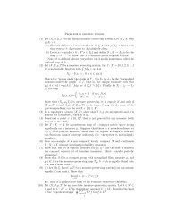
2. For every n, d, ||P d,n || ∞ = 1.<strong>The</strong> Chebyshev polynomials <strong>of</strong> the first kind are defined as T n := P 2,n . <strong>The</strong> Chebyshevpolynomials <strong>of</strong> the second kind are the polynomials over [−1, 1] defined by the recursionformulaU n (x) = 2xU n−1 (x) − U n−2 (x)U 0 ≡ 1, U 1 (x) = 2xWe shall make use <strong>of</strong> the following properties <strong>of</strong> the Chebyshev polynomials.Proposition 5.9 1. For every n ≥ 1, T ′ n = nU n−1 .2. ||U n || ∞ = n + 1.Given a measure µ over [−1, 1], the orthogonal polynomials corresponding to µ are the sequence<strong>of</strong> polynomials obtained upon the Gram-Schmidt procedure applied to 1, x, x 2 , x 3 , . . ..We note that the 1, √ 2T 1 , √ 2T 2 , √ 2T 3 , . . . are the orthogonal polynomials corresponding tothe probability measure dµ =dxπ √ 1−x 25.1.5 Bochner Integral and Bochner SpacesPro<strong>of</strong>s and elaborations on the material appearing in this section can be found in (KosakuYosida, 1963). Let (X, m, µ) be a measure space and let H be a Hilbert space. A functionf : X → H is (Bochner) measurable if there exits a sequence <strong>of</strong> function f n : X → H suchthat• For almost every x ∈ X, f(x) = lim n→∞ f n (x).• <strong>The</strong> range <strong>of</strong> every f n is countable and, for every v ∈ H, f −1 (v) is measurable.A measurable function f : X → H is (Bochner) integrable if there exists a sequence <strong>of</strong> simplemeasurable functions (in the usual sense) s n such that lim n→∞∫X ||f(x)−s n(x)|| H dµ(x) = 0.We define the integral <strong>of</strong> f to be ∫ X fdµ = lim n→∞∫sn dµ, where the integral <strong>of</strong> a simplefunction s = ∑ ni=1 1 A iv i , A i ∈ m, v i ∈ H is ∫ X sdµ = ∑ ni=1 µ(A i)v i .Define by L 2 (X, H) the Kolmogorov quotient (by equality almost everywhere) <strong>of</strong> allmeasurable functions f : X → H such that ∫ X ||f||2 Hdµ < ∞.<strong>The</strong>orem∫5.10 L 2 (X, H) in a Hilbert space w.r.t. the inner product 〈f, g〉 L 2 (X,H) =〈f(x), g(x)〉 X Hdµ(x)5.2 Learnability implies small radius<strong>The</strong> purpose <strong>of</strong> this section is to show that if X is a subset <strong>of</strong> some Hilbert space H suchthat it is possible to learn affine functionals over X w.r.t. some loss, then we can essentiallyassume that X is contained is a unit ball and the returned affine functional is <strong>of</strong> norm O (m 3 ),where m is the number <strong>of</strong> examples.19
Lemma 5.11 (John’s Lemma) (Matousek, 2002) Let V be an m-dimensional real vectorspace and let K be a full-dimensional compact convex set. <strong>The</strong>re exists an inner product onV so that K is contained in a unit ball and contains a ball <strong>of</strong> radius 1 , both are centered atm(the same) x ∈ K. Moreover, if K is 0-symmetric it is possible to take x = 0 and the ratiobetween the radiuses can be improved to √ m.Lemma 5.12 Let l be a convex surrogate, let V an m-dimensional vector space and letX ⊂ V be a bounded subset that spans V as an affine space. <strong>The</strong>re exists an inner product〈·, ·〉 on V and a probability measure µ N such that• For every w ∈ V, b ∈ R, ||w|| ≤ 4m 2 Err µN ,hinge(Λ w,b )• X is contained in a unit ball.Pro<strong>of</strong> Let us apply John’s Lemma to K = conv(X ). It yields an inner product on V withK contained in a unit ball and containing the ball with radius 1 both centered at the samemx ∈ V . It remains to prove the existence <strong>of</strong> the measure µ N . W.l.o.g., we assume that x = 0.Let e 1 , . . . , e m ∈ V be an orthonormal basis. For every i ∈ [m], represent both 1 e m i and− 1 e m i as a convex combination <strong>of</strong> m + 1 elements from X :Now, definem+11m e ∑i =j=1λ j i xj i , − 1 m e i =m+1∑j=1ρ j i zj i .µ N (x j i , 1) = µ N(x j i , −1) = λj i4m , µ N(z j i , 1) = µ N(z j i , −1) = ρj i4m .20
- Page 1 and 2: The complexity of learning halfspac
- Page 3 and 4: exists an equivalent inner product
- Page 5 and 6: is enough that we can efficiently c
- Page 7 and 8: our terminology, they considered th
- Page 9 and 10: It is shown in (Birnbaum and Shalev
- Page 11 and 12: We now expand on this brief descrip
- Page 13 and 14: and (uniformly and independently) a
- Page 15 and 16: The proof of Theorem 2.7To prove Th
- Page 17 and 18: attempts to prove a quantitative op
- Page 19: 5.1.3 Harmonic Analysis on the Sphe
- Page 23 and 24: For 1 ≤ i ≤ t Let v i = x i −
- Page 25 and 26: ( )that in this case Err µN ,hinge
- Page 27 and 28: Thus, it is enough to find a neighb
- Page 29 and 30: Legendre polynomials we have|P d,n
- Page 31 and 32: Then, for every K ∈ N, 1 8 > γ >
- Page 33 and 34: Now, it holds that∫∫∫ ∫∫
- Page 35 and 36: We note that ω f◦g ≤ ω f ·
- Page 37 and 38: Now, denote δ = ∫ g. It holds th
- Page 39 and 40: equivalent formulationminErr D,l (f
- Page 41 and 42: Denote ||g|| Hk = C. By Lemma 5.25,
- Page 43 and 44: Consequently, every approximated so
- Page 45: Kosaku Yosida. Functional Analysis.