The error rate of learning halfspaces using kernel-SVM

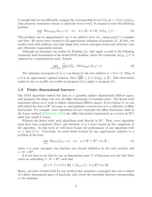
is enough that we can efficiently compute the corresponding kernel, k(x, y) := 〈ψ(x), ψ(y)〉 H1(this property, sometimes crucial, is called the kernel trick). It remains to solve the followingproblemminw,bErr D,hinge (Λ w,b ◦ ψ) s.t. w ∈ H 1 , b ∈ R, ‖w‖ H1 ≤ C . (2)This problem can be approximated, up to an additive error of ɛ, using poly(C/ɛ) samplesand time. We prove lower bounds to all approximate solutions of program (2). In fact, ourresults work with arbitrary (not just hinge loss) convex surrogate losses and arbitrary (notjust efficiently computable) kernels.Although we formulate our results for Problem (2), they apply as well to the followingcommonly used formulation of the kernel SVM problem, where the constraint ‖w‖ H1 ≤ C isreplaced by a regularization term. Namelyminw∈H 1 ,b∈R1C 2 ‖w‖2 H 1+ Err D,hinge (Λ w,b ◦ ψ) (3)The optimum of program (3) is ≤ 1 as shown by the zero solution w = 0, b = 0. Thus, ifw, b is an approximate optimal solution, then ‖w‖2 H 1C 2 ≤ 2 ⇒ ‖w‖ H1 ≤ 2C. This observationmakes it easy to modify our results on program (2) to apply to program (3).1.3 Finite dimensional learnersThe SVM algorithms embed the data in a (possibly infinite dimensional) Hilbert space,and minimize the hinge loss over all affine functionals of bounded norm. The kernel tricksometimes allows us to work in infinite dimensional Hilbert spaces. Even without it, we canstill embed the data in R m for some m, and minimize a convex loss over a collection of affinefunctionals. For example, some algorithms do not constraint the affine functional, while inthe Lasso method (Tibshirani, 1996) the affine functional (represented as a vector in R m )must have small L 1 -norm.Without the kernel trick, such algorithms work directly in R m . Thus, every algorithmmust have time complexity Ω(m), and therefore m is a lower bound on the complexity ofthe algorithm. In this work we will lower bound the performance of any algorithm withm ≤ poly (1/γ). Concretely, we prove lower bounds for any approximate solution to aproblem of the formminw,bErr D,l (Λ w,b ◦ ψ) s.t. w ∈ W ⊂ R m , b ∈ R , (4)where l is some surrogate loss function (see formal definition in the next section) andψ : B → R m .It is not hard to see that for any m-dimensional space V of functions over the ball, thereexists an embedding ψ : B → R m such that{f + b : f ∈ V, b ∈ R} = {Λ w,b ◦ ψ : w ∈ R m , b ∈ R}Hence, our lower bounds hold for any method that optimizes a surrogate loss over a subsetof a finite dimensional space of functions, and return the threshold function correspondingto the optimum.4