Homework 2 (Attendance 3) for Statistics 512 Applied Regression ...

More documents

Recommendations

Info

(b) The residual plot of e versus Ŷ indicates (choose one) more or less constant/ badly varying variance.elapsed time, X 16 16 16 · · · 40 40hardness, Y 199 205 196 · · · 253 246predicted, Ŷ 201.15 201.15 201.15 · · · 249.98 249.98residual, e = Ŷ − Y -2.15 3.85 -5.15 · · · 3.025 -3.975(2nd STAT PLOT, ON, choose scatter plot of L 3 and L 4 .)(c) From SAS,ordered residual, e -5.150 -3.975 · · · 3.850 5.575expected residual, E[e] = √ MSE [ z ( )]k−0.375-5.720 -4.145 · · · 4.145 5.720n+0.25First, the normal probability plot of the residuals versus the expectedresiduals is more or less linear and so indicates the residuals are normal/ not normal.Second, the correlation test for the normal probability plot is given by,1. Statement.The statement of the test is (check none, one or more):(i) H 0 : ρ = 1 versus H 1 : ρ > 1.(ii) H 0 : ρ = 1 versus H 1 : ρ < 1.(iii) H 0 : ρ = 1 versus H 1 : ρ ≠ 1.Recall that if ρ = 1, this implies that the scatterplot is linear. Also recallif the normal probability plot is linear, this indicates the residualsare normally distributed.2. Test.From SAS, the test statistic is(choose one) 0.786 / 0.901 / 0.992The critical value at α = 0.05 and n = 20, is(circle one) 0.322 / 0.941 / 0.951(use Table B.6 of the Neter et al. text)3. Conclusion.Since the test statistic is smaller / larger than the critical value we(circle one) accept / reject the null hypothesis that ρ = 1.(d) From the SAS output, a list the semistudentized residuals are given by,ordered residual, e -5.150 -3.975 · · · 3.850 5.575studentized residual, e ∗ = √ eMSE-1.592 -1.229 · · · 1.190 1.724The 25th, 50th and 75th t percentiles and corresponding cumulative frequenciesfrom the e ∗ above are:
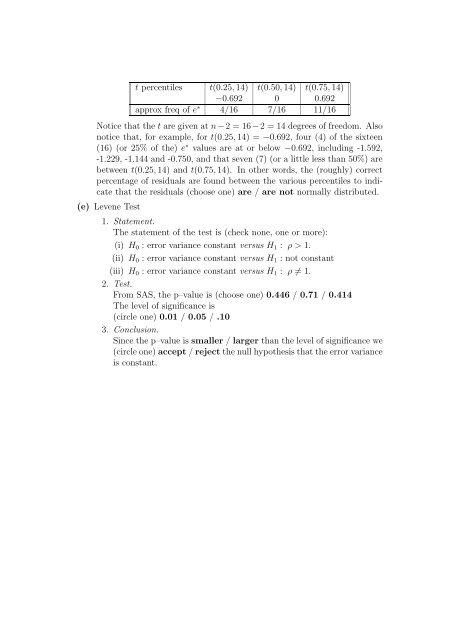
t percentiles t(0.25, 14) t(0.50, 14) t(0.75, 14)−0.692 0 0.692approx freq of e ∗ 4/16 7/16 11/16Notice that the t are given at n − 2 = 16 − 2 = 14 degrees of freedom. Alsonotice that, for example, for t(0.25, 14) = −0.692, four (4) of the sixteen(16) (or 25% of the) e ∗ values are at or below −0.692, including -1.592,-1.229, -1.144 and -0.750, and that seven (7) (or a little less than 50%) arebetween t(0.25, 14) and t(0.75, 14). In other words, the (roughly) correctpercentage of residuals are found between the various percentiles to indicatethat the residuals (choose one) are / are not normally distributed.(e) Levene Test1. Statement.The statement of the test is (check none, one or more):(i) H 0 : error variance constant versus H 1 : ρ > 1.(ii) H 0 : error variance constant versus H 1 : not constant(iii) H 0 : error variance constant versus H 1 : ρ ≠ 1.2. Test.From SAS, the p–value is (choose one) 0.446 / 0.71 / 0.414The level of significance is(circle one) 0.01 / 0.05 / .103. Conclusion.Since the p–value is smaller / larger than the level of significance we(circle one) accept / reject the null hypothesis that the error varianceis constant.
Page 1 and 2: Homework 2 (Attendance 3) for Stati
Page 3 and 4: *3.3(D) NORMAL PROBABILITY PLOT AND
Page 6 and 7: (3.6) plastic hardness, hw2-3-6-pla
Page 10 and 11: (3.14) More Plastic hardness, lack
Page 12 and 13: (3.15) Solution concentration, lack
Page 14 and 15: (3.16) Solution concentration, tran
Page 16: (a) The scatter plot suggests which

Homework 2 (Attendance 3) for Statistics 512 Applied Regression ...

Create successful ePaper yourself

Delete template?

Save as template?