1 Quiz Practice Questions 4 (Attendance 8) for Statistics 513 ...

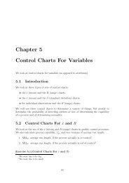
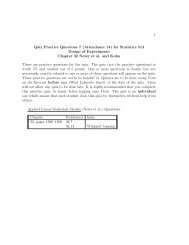
1Quiz Practice Questions 4 (Attendance 8) for Statistics 513Statistical Control TheoryMaterial Covered: Chapter 9 Montgomery and KuhnBy: Friday, 12th March, Spring 2004These are practice questions for the quiz. The quiz (not the practice questions) isworth 5% and marked out of 5 points. One or more questions is closely, but notnecessarily exactly, related to one or more of these questions will appear on the quiz.These practice questions are not to be handed in. Quizzes are to be done using Vistaon the Internet before 4am of the date of the quiz. Vista will not allow any quizto be done late. It is highly recommended that you complete this practice quiz, byhand, before logging onto Vista. The quiz is an individual one which means thateach student does this quiz by themselves without help from others.Introduction to Statistical Control Theory (Montgomery) Questions.Chapter Problem(s) hints9, pages 499–506 9-29-69-89-109-169-189-28

Practice Quiz Questions 4 (Attendance 6), 9-2, pp 499–506 2(9-2) Small run chart or standardized DNOM: qz4-9-2-part-DNOMX chartFrom SAS, the standardized DNOM ¯x chart for the three parts is out ofstatistical control for ?R chartThe standardized DNOM R chart for the three parts is(choose one) in / out of statistical control.

Practice Quiz Questions 4 (Attendance 6), 9-6, pp 499–506 3(9-6) Multiple stream process: qz4-9-6-heads-groupOriginal dataFrom SAS, the ¯x chart for the maximum of the four heads is out of statisticalcontrol, although it is not possible to tell from the charts whether any particularhead is out of statistical control. That all heads, together, seem out of control,is confirmed by looking carefully at the data itself.Also, the both ¯x chart and corresponding listed data for the minimumof the four heads is out of statistical control, although, again, it does not seemto be the case that any particular head is out of statistical control.The R chart, on the other hand, appears to be in statistical control.New dataFrom SAS, it appears the new data is, if anything, more out of statisticalcontrol than the original data. In particular, the ¯x chart for the maximum ofthe four heads looks further out of statistical control (above UCL) than before.Looking carefully at the data itself, it looks like head ?, in particular, is themain cause of being out of statistical control.The R chart now appears to be out of statistical control because all ofthe data falls above the centerline.

Practice Quiz Questions 4 (Attendance 6), 9-8, pp 499–506 4(9-8) Modified chart and acceptance chart: qz4-9-8-product-modified(a) Modified control chart, α = 0.01Since the specifications are (LSL, USL) = 0.55 ± 0.02 = (0.53, 0.57)and since 1 δ = 0.01, Z δ = Z 0.01 = 2.326, n = 5and, from SAS, ¯x = 0.55025, ¯R = 0.00227 then ˆσ =¯Rd 2= 0.0227 = 0.00201.128and so(LCL, UCL) =(= ?LSL +(Z δ − 3 √ n)σ, USL −(Z δ − √ 3 ) )σ n(b) Acceptance control chart, γ = 0.01, 1 − β = 0.90Since the specifications are (LSL, USL) = 0.55 ± 0.02 = (0.53, 0.57)and since γ = 0.01, Z γ = Z 0.01 = 2.326and 1 − β = 0.90, Z β = Z 0.10 = 1.28and n = 5and, from SAS, ¯x = 0.55025, ¯R = 0.00227 then ˆσ =¯Rd 2= 0.0227 = 0.00201.128and so( (()(LCL, UCL) == ?LSL +Z γ + Z β√ n)σ, USL −Z γ + Z β√ n)σThe acceptance chart has slightly narrower (smaller) control limits thanthe previous modified chart control limits.1 The value Z 0.01 is calculated using 2nd DISTR InvNorm(0.99) ENTER.

Practice Quiz Questions 4 (Attendance 6), 9-10, pp 499–506 5(9-10) Acceptance chart, sample sizeSince δ = 0.001, Z δ = Z 0.001 = 3.090and α = 0.05, Z α = Z 0.05 = 1.645and γ = 0.02, Z γ = Z 0.02 = 2.054and β = 0.10, Z β = Z 0.10 = 1.282and son =( ) 2Zα + Z βZ δ − Z γ= ?

Practice Quiz Questions 4 (Attendance 6), 9-16, pp 499–506 6(9-16) Time series, 1st order autoregressive model: qz4-9-16-mole-firstorderauto(a) Sample autocorrelationThe sample autocorrelation at lag 1 is r 1 = ?. Since this statistic appear tobe significant at two standard deviations, this indicates that a first–orderautoregressive model, AR(1 ), might be appropriate for the data.The sample autocorrelation at lag 2 is r 2 = 0.373 and also appearsto be at least close to significant at two standard deviations. This impliesa second–order autoregressive model, AR(2 ), might also be appropriate,but, nonetheless, we will stick with the AR(1 ) model.(b) Individual control chartThe individual x chart (and, to some extent, the R chart) indicates thatthe process is out of control for a number of measurements. However, weknow that these out of control signals are probably due to the significantpositive correlation at lag 1.(c) First–order autoregressive model, AR(1 )From SAS, the approximate AR(1 ) model is given byˆx t = ˆξ + ˆφx t−1 = ? + ?x t−1The residual plot, e t = x t − ˆx t , indicates the residuals are in control, withthe exception of one out of control residual at around 15.

Practice Quiz Questions 4 (Attendance 6), 9-18, pp 499–506 7(9-18) EWMA approximation to time series: qz4-9-18-mole-ewma,ar1Ewma chart for residualsLet λ = 0.1, L = 3and, from SAS, µ 0 ≈ ¯x residuals = −0.4118, σ 0 ≈ s residuals = 20.74So, from the ewma chart produced by SAS for the residuals for the AR(1 )model, it appears as though the residuals are in statistical control.Moving center line ewma control chart for weightsLetz t = λx t + (1 − λ)z t−1be the center line on a control chart and define the control limits as(LCL t+1 , UCL t+1 ) = x t ± 3σAccording to this chart, the process appears to be in statistical control.Comparing the two charts?

Practice Quiz Questions 4 (Attendance 6), 9-28, pp 499–506 8(9-28) Moving range approximation to time series and estimation of standard deviation(a) Estimation of standard deviationWhen the data are positively autocorrelated, adjacent observations willtend to be similar, therefore making the moving ranges (choose one)smaller / larger. This would tend to produce an estimate of the processstandard deviation that is too (choose one) small / large.(b) More estimation of standard deviationS 2 is still an unbiased estimator of σ 2 when the data are positively autocorrelated.(c) More on estimation of standard deviationIf assignable causes are present, it is not good practice to estimate S 2with σ 2 . Since it is difficult to determine whether a process generatingautocorrelated data– or really any process–is in control, it is generally abad practice to estimate S 2 with σ 2 .