Robust Height Tracking by Proper Accounting of ... - Xsens

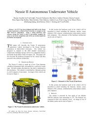
S ω LS∫LS q 0LS qaccelerometer measurement noise. They are assumed to bezero mean independently and identically distributed (i.i.d.)Gaussian noisesS e ω ∼ N (0, Σ eω ), (3)L v 0 L vS f L f remove L arotategravity∫∫L p 0L pS e a ∼ N (0, Σ ea ), (4)where Σ eω and Σ ea are the covariance matrix of the measurementnoises of the angular velocity and the acceleration,respectively.Fig. 1. Strapdown inertial integration, the orientation LS q is expressed usingquaternion, the velocity L v and the position L p are obtained by the deadreckoning from the initial condition and the inertial measurements, angularvelocity S ω LS and specific force S f.includes the strapdown inertial integration, the UWB systemand the barometer. In section III, the system model andthe nonlinearity problem are formulated, section IV explainsthe experiment setup and the estimation results are analyzedand compared with an accurate reference system. Finallyconclusions are presented in section V.II. SYSTEM OVERVIEWThe integrated system includes two components: a low-cost,low-form factor MEMS IMU consisting a three dimensional(3D) rate gyroscope and a 3D accelerometer which incorporatesa barometer on the board, and a UWB system. In thissection we will introduce each technology and their modelingfor positioning purpose.A. Strapdown inertial integrationIn inertial sensors, the accelerometers measure externalspecific force in the imu frame (S-frame), denoted as S f.Gyroscopes measure the angular velocity from the S-frame tothe inertial frame (I-frame) expressed in the S-frame, S ω IS .In order to keep the discussion simple, we apply correctionterms which allow us to write the gyroscope measurementusing the angular velocity from the S-frame to the localframe (L-frame) expressed in the S-frame, S ω LS . The inertialnavigation solution calculates the current position and orientationof an object from an initial condition by integratingthe information obtained from the inertial sensors which iscommonly referred to as strapdown inertial integration or deadreckoning [1], as shown in Figure 1.The inertial measurement model can then be written asy gyr = S ω LS + S b ω + S e ω , (1)y acc = S f + S b a + S e a = SL R( L a − L g) + S b a + S e a ,(2)where SL R denotes the rotation matrix from the L-frame tothe S-frame. L a represents the acceleration in the L-frameobtained by the specific force L f subtracting the gravityL g in the L-frame. S b ω is the gyroscope bias and S b a isthe accelerometer bias. They are slow time-varying biases.S e ω is the gyroscope measurement noise and S e a is theB. BarometerThe barometer measures the atmospheric pressure. Theknowledge that air pressure decreases with increase in altitudecan be used to get the height information [14]. From thepressure output of the barometer, the change in height withrespect to an initial height can be obtained [10]. The absolutealtitude can be calculated from the measured pressure usingthe international barometric formula [15]h = 44330 × (1 − ( P P 0) 5.255 ), (5)where P is the measured pressure in Pascal, P 0 is the pressureat sea level, and the altitude h is in meters. P 0 is approximately101.325 kPa under normal conditions, but it varies as theweather changes. Since we want to estimate the height in theL-frame and not the absolute altitude with respect to the sealevel, we can model the barometer measurements asy baro = L p z + b baro + e b , (6)where L p z is the position in z direction, i.e., height in the L-frame. b baro represents the barometer baseline used to modelthe initial height, the calibration bias and the atmosphericpressure fluctuation due to the unstable weather. This issimilar to using a reference barometer presented in [10]. Themeasurement noise e b is assumed to be zero mean Gaussiannoisee b ∼ N (0, σ 2 e b), (7)which accounts for the thermal noise and the quantizationnoise. The typical value of σ eb for the barometer we use isapproximately 0.5 m. It is apparent that the drawback of thebarometer is its coarse height measurement. The advantageof using the barometer is that it provides long-term stabilitywhich can be used to limit the drift in the vertical channelestimates of the inertial sensors.C. UWBUWB systems have the potential to provide high-precisionpositioning due to their large bandwidth, which results inhigh time resolution. There are various parameters that canbe extracted from the radio signals travelling between differentnodes that can be used to calculate the node positions, such astime of arrival (TOA), angle of arrival (AOA), and received signalstrength (RSS). The UWB system used for our experimentscalculates the ranges between pairs of nodes based on the time1

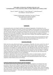
of flight (TOF) estimated by a two-way ranging protocol [6].These ranges can be modelled as:y ri = ‖ L p ri − L p‖ 2 + e r , i = 1, 2, ..., n, (8)where ‖.‖ 2 is the Euclidean distance, L p represents theposition of the target node to be tracked, and L p ri denotesthe position of a reference node r i . Note that in contrast toGPS, the ranges from a target node to the reference nodesare estimated sequentially. The reference nodes are assumedstationary with known positions. For a 3D tracking system,at least four reference nodes are required to obtain a uniqueposition. However, if the constraint that the target node mustlie on one side of the reference nodes can be applied, threereference nodes are sufficient for a 3D localization. Themeasurement noise e r is assumed to be zero mean Gaussiannoisee r ∼ N (0, σe 2 r). (9)However, when the target node moves close to the floor, wallsor ceiling, due to the multipath and NLOS propagation, outliersappear that affect the range accuracy resulting in a seriousdegradation of range accuracy.Another factor influencing the positioning accuracy is theposition dilution of precision (PDOP), i.e., the geometry of thereference nodes and the target node. For a trilateration systemas defined by (8), the expected positioning error consists twoparts: the range measurement error σ er and the PDOP factorRMSEpos = PDOP · σ er , (10)where RMSEpos represents the root mean square error(RMSE) of the position estimate. The PDOP is then definedas√σx 2 + σy 2 + σz2PDOP =, (11)σ erAs shown in (10), a PDOP greater than one will degradethe positioning accuracy. That is, a higher value of PDOPmeans a poor geometry, whereas a lower value indicates abetter geometry. The VDOP is calculated using (11) but onlytaking account of the vertical position error σ z . The PDOP isonly affected by the geometrical configuration of the referencenodes and the target node, and it can be therefore predictedfor a given constellation and a specified position of the targetnode√PDOP = tr((H T H) −1 ), (12)where H is the Jacobian matrix of the Euclidean distance asgiven in (8).III. PROBLEM STATEMENTAs the inertial sensor provides short-term accurate angularrate and acceleration with high data rate, it can be usedto model the dynamics of the target, while the UWB rangemeasurements and the barometer height measurements areused to correct the dead reckoning results. The hybrid trackingsystem can be written as a discrete-time nonlinear state spacemodelx k+1 = f(x k , w k ), (13)y k = h(x k , v k ), (14)where the noises are modelled as zero mean Gaussian noisesw k ∼ N (0, Q k ), (15)v k ∼ N (0, R k ). (16)The states to be estimated are the orientation,LS q, thegyroscope bias, S b ω , the accelerometer bias, S b a , the velocityin the L-frame, L v, the position in the L-frame, L p, and thebarometer baseline, b baro . The state vector is given byx = [ LS q S b ω S b a L v L p b baro] T, (17)where we also estimate the barometer baseline for better trackingthe barometer measurement fluctuation as the atmosphericconditions change. The system model is then given by:System Model:whereLS q k+1 = LS q k ⊙ exp( T S 2ω LS,k ),S b ω,k+1 = S b ω,k + w bω ,S b a,k+1 = S b a,k + w ba ,L v k+1 = L v k + T L a k ,L p k+1 = L p k + T L v k + T 2 L a k ,b baro,k+1 = b baro,k + w bbaro ,2(18a)(18b)(18c)(18d)(18e)(18f)L a k = LS q k ⊙ S f k ⊙ LS q c k + L g. (19)The orientation is represented by quaternion [16], LS q is therotation from the S-frame to the L-frame. (19) denotes a vectorrotation using quaternion multiplication, ⊙, and the superscriptc is the quaternion conjugation operation. Here we model thegyroscope bias, accelerometer bias and the barometer baselineas random walk.Measurement Model:y ri,k = ‖ L p ri − L p k ‖ 2 + e r , , i = 1, 2, ..., n, (20)y baro,k = L p z,k + b baro,k + e b , (21)In the above system, the nonlinearity when rotating thespecific force vector (19) is problematic since it always resultsin a downward bias in the vertical channel. As explained in [9],the probability density function of the rotated acceleration isnot a Gaussian shape, but rather like an umbrella, see Figure 2.We have demonstrated this umbrella-shaped nonlinearity of theinertial strapdown integration in the previous work [9] usingMEMS inertial data. As the orientation uncertainty increases,the resulting rotated acceleration will have a large bias invertical direction. This results in a quadratically growingdownward position error by double integration. It has beenshown that the first order Taylor linearization does not modelthis bias, whereas the second order expansion models thisumbrella-shaped nonlinearity more accurately. By successfully

Rotated Acceleration (X−Z View)Range [m]5432Ref. Node 1Ref. Node 2Ref. Node 3Ref. Node 4Ref. Node 5Range Measurementsa z[m/s 2 ]1Outliers00 1 2 3 4 5Time [s]Fig. 3. Illustration of the UWB range data from five reference nodes duringa static period. Some of the outliers present in the range measurements arehighlighted in the figure.a x[m/s 2 ]15Histogram of Range ErrorFig. 2. Umbrella problem illustration (X-Z view) [9]. The arrow denotesan vector to be estimated, the rotated vector (the dots) due to a Gaussiandistributed orientation error is distributed like an umbrella.applying the EKF2 (prediction part) for the strapdown inertialintegration, we obtain an improved height prediction ascompared to a normal EKF. Therefore, applying this approachin the integration of inertial sensors with position aiding isanticipated to improve the height estimate due to a bettermodeling in the height direction. We will demonstrate thisapproach in the following section.A. System setupIV. EXPERIMENTAL RESULTSFor the purpose of demonstration we here choose an indoorexperimental setup. Five UWB reference nodes are placedin known locations inside a room with a relatively goodgeometric configuration.The unit to be tracked contains a UWB target node rigidlyconnected to a motion tracker, i.e., the inertial sensor unit. Foranalysing the performance of the tracking system, we use ahigh-precision optical motion capture system to get an accurateand reliable position reference, with which we compare theperformance of our approaches. The motion tracker data arecollected at a high rate of 100 Hz, the barometer providesheight information at 50 Hz, and the UWB measures theranges in the way of ’One Shot’ ranging with each referencenode in turn. The range update is about 10 Hz in total, withrange to each reference node estimated in turn at a rate ofapproximately 2 Hz as shown in Figure 3. All ranges are timestampedusing the internal clock of the target node. Figure 4shows a typical error histogram of the range data complying toa zero mean Gaussian distribution with the standard deviationof about 0.1 m in the absence of outliers. However, the outliershappen often when the target node moves close to the floor,the ceiling, or is occluded by the body. For demonstrationpurposes, we remove the UWB outliers greater than 4σ er basedon the optical truth reference. We note that the problem ofoutlier detection itself is outside the scope of this paper. TheError Count1050−0.5 0.1 0 0.1 0.5Range Error [m]Fig. 4. Typical error histogram of the UWB range data. The outliers presentin the range measurements as shown in Figure 3 make the noise distributionnon-gaussian.systems are all synchronized and aligned either in hardwareor through data postprocessing.The following two scenarios are used to demonstrate theproposed system’s performance:• Normal height tracking in human motion: the motiontracker moves randomly and the height varies in time.• Sensor saturation: the gyroscope measurement from themotion tracker IMU saturates at times during the trial.The following are the different integrated solutions used inthe analyses:• EKF with baro - the solution of the UWB, barometer andIMU in an EKF framework.• EKF without baro - the solution of the UWB and IMU inan EKF framework.• EKF2 with baro - is the proposed system under test.The solution of the UWB, barometer and IMU in an EKF2framework.• EKF2 without baro - the solution of the UWB and IMUin an EKF2 framework.B. Test 1: normal height tracking in human motionThe test is to demonstrate that the proposed integrated systemof the inertial sensor, the UWB system and the barometerprovides smooth tracking and in particular can track the heightaccurately. For this test, the trajectory is chosen in the space

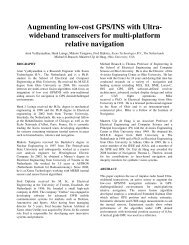
2.52Height EstimateEKF with Baro (estimating baro baseline)EKF with Baro (not estimating baro baseline)EKF without BaroTruth1.5Position z [m]10.50−0.50 10 20 30 40 50 60 70 80 90Time [s]Fig. 6. Test 1: the height estimate (dashed) using EKF as compared with the true position (solid). The height estimate of an EKF without barometer (dotted)and that of an EKF with barometer but without estimating the barometer baseline (gray dash-dot) are also plotted.21.5DOPsTABLE IRMSES FOR TEST 1Approaches RMSE in x RMSE in y RMSE in zEKF with Baro (baseline) 0.14 m 0.15 m 0.13 mEKF with Baro (no baseline) 0.23 m 0.17 m 0.41 mEKF without Baro 0.14 m 0.15 m 0.19 m10.50 10 20 30 40 50 60 70 80 90Time [s]Fig. 5. DOPs during tracking, where the plots represent the DOPs in differentdirections (red dash-dot: x; green dashed: y; blue solid: z).with a relatively good PDOP. As shown in Figure 5, however,the VDOP is still relatively poor being twice as bad as thanthat of the horizontal DOP components. Figure 6 shows theheight estimate using the approach of EKF with barometer andestimating the barometer baseline, that of EKF with barometerbut without estimating the barometer baseline, and that ofEKF without barometer, respectively. As compared to the trueposition, the EKF with baro and estimating barometer baselinetracks the target continuously and accurately. As shown inFigure 3, there are usually no sufficient ranges in a single timeinstant and many ranging failures (gaps) in the data series. Itis therefore difficult for the UWB system alone to calculatea unique position at each time and provide a continuoustrajectory. In contrast, the integration of the inertial sensorand the UWB use all the information and can fill the gapsto provide smooth tracking. Moreover, the barometer addsadditional values to stabilize the height estimate. Comparingthe height estimate applying the barometer and the estimatewithout the barometer, the estimation accuracy is improved. Itcan be seen clearly from Table I that the integration schemeincluding the barometer baseline as a state performs the best.The incorporation of the barometer baseline as a state furtherhelps the tracking since an arbitrary baseline value results inheight bias when the atmospheric conditions change duringthe trial. Without the barometer baseline as a state, the erroris greater than without the barometer.As introduced, the data rate of the barometer we used is50 Hz. It may be a requirement to decrease the data rate toreduce the data load. Figure 7 gives the RMSEs for differentbarometer data rates. The height RMSE increases as the datarate decreases while the RMSEs in other channels stay atapproximately the same level. It is noticed that the heightRMSE increases and reaches a value in the low frequencywhich is close to the RMSE without using the barometer, seeTable I. Without barometer the height RMSE is apparentlyworse than the horizontal RMSEs due to the worse VDOP. TheRMSEs of the EKF2 are also plotted in Figure 7. It should bestressed that the EKF2 performs similar to the EKF here sincethe nonlinearity of the acceleration rotation is not prevalentfor this test due to the high data rate of the inertial sensor.

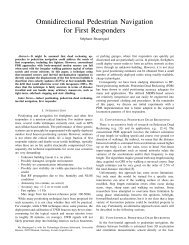
RMSE [m]0.190.180.170.160.15RMSE in x (EKF)RMSE in y (EKF)RMSE in z (EKF)RMSE in x (EKF2)RMSE in y (EKF2)RMSE in z (EKF2)RMSEs of EstimateTABLE IIRMSES FOR TEST 2Approaches RMSE in x RMSE in y RMSE in zEKF with Baro 0.27 m 0.19 m 0.16 mEKF2 with Baro 0.22 m 0.15 m 0.13 mEKF without Baro 1.23 m 1.18 m 1.35 mEKF2 without Baro 0.43 m 0.31 m 0.54 m0.140.1350 20 10 5 2 1 1/2Barometer Data Rate [Hz]Fig. 7. The RMSEs of the EKF and EKF2 against different barometerdata rates. Height estimation accuracy decreases as barometer update ratedecreases. Both EKF and EKF2 achieve similar performance as there are nosubstantial nonlinearities during the trial.Angular Velocity [rad/s]3020100−10−20Gyroscope Signalsx Channely Channelz Channel−3042.8 42.9 43 43.1 43.2 43.3 43.4 43.5 43.6Time [s]Fig. 8. Illustration of sensor saturation. The gyroscope saturates in thez channel (solid). During such a period, the angular velocity output of thegyroscope is not representative of the true motion performed.C. Test 2: sensor saturationThis test is to prove the robust performance of the EKF2as compared to a normal EKF in the case of high nonlinearitywhen the orientation uncertainty is large. Figure 8 illustratesthe gyroscope saturation, where the gyroscope outputs a constantvalue when the sensor is rotated exceeding an angularvelocity threshold, here 27.92 rad/s or 1600 ◦ /s. That is, thegyroscope signal does not give the realistic angular velocitywhich is much higher than we receive from the sensor.As derived in [9], the acceleration rotation (19) can belinearized using the 1 st and 2 nd order Taylor expansion. Herewe split the orientation LS q ( LS R) into a nominal orientationLS¯q ( LS ¯R) and an orientation error S θ,LS q = LS¯q ⊙ exp(− 1 S 2θ). (22)Given the random variables, the orientation error S θ ∼N (µ S θ, Σ S θ), the specific force S f ∼ N (µ S f , Σ S f ) andchoosing the linearization point at S¯θ = µ S θ = 0, we obtainthe mean and covariance of the linearized functionE{f 1st } = LS ¯Rµ S f + L g, (23)Cov{f 1st } = [D θ f] S¯θΣ S θ [D θ f] T S¯θ+ LS ¯RΣ S f LS ¯RT ,(24)andE{f 2nd } = LS ¯Rµ S f + L g+ 1 2[tr([Hθθ f] S¯θ,iΣ S θ) ] i , (25)Cov{f 2nd } = [D θ f] S¯θΣ S θ [D θ f] T S¯θ+ LS ¯RΣ S f LS ¯RT[+ 1 tr([Hθθ f]2S¯θ,iΣ S θ [H θθ f] S¯θ,jΣ S θ) ] , ij(26)where tr(·) is the matrix trace operation. [x i ] idenotes a vectorwhose i th element is x i , and [x ij ] ijdenotes a matrix whoseij th element is x ij . [D θ f] denotes the Jacobian matrix and[H θθ f] represents the Hessian matrix [17]. The details of thederivation can be found in [9]. The EKF and EKF2 provide themean and the covariance estimate as (23) (24) and (25) (26),respectively. Comparing (23) and (25), it can be anticipatedthat when the additional term representing the orientationuncertainty in (25) is significant, the estimate of EKF andEKF2 will have a difference and the EKF2 can compensate thebias caused by this large orientation error, like in the situationof the gyroscope saturation. In such situation, the normalEKF only models the nonlinearity using the first order Taylorexpansion, whereas the EKF2 can approximate it accuratelyusing the second order expansion due to the bilinear nature ofthis nonlinearity. However, when the additional term is trivial,like in test 1, the high frequency of the motion tracker makesthe linearization point LS ¯R close to the true orientation, theEKF and EKF2 will output similar performance.Figure 9 shows the height estimate obtained by the EKFand the EKF2, with and without barometer, respectively, ascompared to the true position. The performance of the filterscombined with the barometer is generally better than the filterswithout using the barometer. The EKF2s are able to providemore robust estimate as compared to the EKF. Even withoutthe barometer aiding, the EKF2 can still converge to the trueheight after the saturation. Table II presents the RMSEs ofdifferent approaches, among which the EKF2 with barometerprovides the best performance.D. Test 3: UWB outageThe final test demonstrates the ability of the filters to handlean outage in the UWB aiding data. The data set from test 1is reused, with a simulated UWB outage lasting ten secondsduring a period of high dynamics. Such outages can occur inpractice due to a wide variety of causes:• occlusion of the line of sight (LOS) path between targetand reference nodes.• rejected measurements due to outlier detection algorithms.

Fig. 9. Test 2: the height estimate (dashed) with the 3σ uncertainty band using different approaches as compared with the true position (solid). Comparingthe upper plots with barometer data to the lower plots without, it is evident that the addition of barometer data greatly improves height estimation duringgyroscopic sensor saturation events. Without barometer data the EKF is liable to diverge, while the EKF2 demonstrates its improved robustness by convergingon the true solution.• poor ranging channel access control leading to datastarvation.• movement out of range of the reference nodes.The ability of the EKF and EKF2 filters, with and withoutbarometer data, to track the height robustly is illustrated inFigure 10. The important difference between the EKF andEKF2 filters is highlighted by the estimated error covariance.For both filters the covariance increases during the outage asinertial integration error accumulates. For the approaches withthe barometer aiding (upper figures), the covariance increasingis limited by the barometer measurement accuracy. Once UWBdata are restored the EKF covariance decreases dramatically,and incorrectly, resulting in degraded performance. This isparticularly evident for the EKF without barometer data wherethe height error jumps to over 15 m. In contrast, the EKF2covariance decreases slower, resulting in improved integrationof the noisy UWB range estimates. This clearly demonstratesthe increased robustness of the EKF2 design.The importance of the barometer in aiding height estimatesis once again demonstrated for both filter types. The barometerdata also reduce the error in the horizontal plane as shown byTable III.V. CONCLUSIONIn this paper, we present an integrated tracking systemconsisting of a MEMS IMU, a UWB system and a barometerfor robust and accurate tracking. It has been demonstratedusing experiments that the incorporation of the barometerhas improved the tracking in the height direction. Moreover,TABLE IIIRMSES FOR TEST 3Approaches RMSE in x RMSE in y RMSE in zEKF with Baro 0.38 m 0.55 m 0.29 mEKF2 with Baro 0.36 m 0.49 m 0.16 mEKF without Baro 0.62 m 0.73 m 0.85 mEKF2 without Baro 0.39 m 0.65 m 0.42 mthe nonlinearity problem of rotating the acceleration is takenaccount by applying an EKF2 and has been proven capable toprovide more robust tracking in the challenging situations ofsensor saturation and prolonged position aiding outage.The improved robustness of the EKF2 is not without limitationshowever. It is still crucial to reliably detect and removeoutliers from the position aiding data. The robustness of theEKF2 lies in its ability to handle aiding data outages by bettermodeling the nonlinearities of the strapdown inertial integration.This potentially allows the use of more conservativeoutlier detection algorithms with higher false positive rates.ACKNOWLEDGMENTThe research leading to these results has received fundingfrom the EU’s Seventh Framework Programme under grantagreement no. 238710. The research has been carried out inthe MC IMPULSE project: https://mcimpulse.isy.liu.se.REFERENCES[1] D. H. Titterton and J. L. Weston, Strapdown Inertial Navigation Technology.Peter Peregrinus Ltd., 1997, IEE radar, sonar, navigation andavionics series.

Fig. 10. Test 3: the height estimate (dashed) with the 3σ uncertainty band using different approaches as compared with the true position (solid) during UWBaiding data outage. During the outage the covariance of the state estimates increases due to integration of inertial data. For the filters aiding by the barometerin the upper figures, the covariance increasing is bounded by the barometer measurement accuracy. Once aiding data is restored, the EKF covariance rapidlydecreases, meaning that incorrect Kalman gain is applied to the aiding data. This is highlighted in the lower left figure where, without barometer data, thepoor EKF covariance estimate results in an unacceptable level of error.[2] P. D. Groves, Principles of GNSS, inertial, and multisensor integratednavigation systems. Atrech House, 2008.[3] A. Vydhyanathan, M. Kok, and K. L. Johnson, “A low-cost navigationsystem: high dynamic flight test results,” in Proc. of The EuropeanNavigation Conference on Global Navigation Satellite Systems, Braunschweig,Germany, Oct. 2010.[4] J. D. Hol, F. Dijkstra, H. Luinge, and T. B. Schön, “Tightly coupledUWB/IMU pose estimation,” in Proc. of IEEE International Conferenceon Ultra-Wideband 2009, Vancouver, Canada, Sep. 2009, pp. 688–692.[5] L. B. M. M. Ghavami and R. Kohno, Ultra-wideband Signals andSystems in Communication Engineering. John Wiley & Sons, 2007.[6] Z. Sahinoglu, S. Gezici, and I. Guvenc, Ultra-wideband PositioningSystems: Theoretical Limits, Ranging Algorithms, and Protocols. CambridgeUniversity Press, 2008.[7] A. Vydhyanathan, H. Luinge, M. Tanigawa, F. Djikstra, M. S. Braasch,and M. Uijt de Haag, “Augmenting low-cost GPS/INS with ultrawidebandtrasceivers for multi-platform relative navigation,” Proceedingsof the 22 nd International Technical Meeting of the SatelliteDivision of the Institute of Navigation (ION GNSS 2009), Savannah,GA, pp. 547–554, Sep. 2009.[8] R. B. Langley, “Dilution of precision,” GPS World, pp. 52–59, May1999.[9] M. Zhang, J. D. Hol, L. Slot, and H. Luinge, “Second order nonlinearuncertainty modeling in strapdown integration using MEMS IMUs,” inProc. of the 14th International Conference on Information Fusion, vol. 1,Chicago, US, Jul. 2011, pp. 1679–1685.[10] M. Tanigawa, H. Luinge, L. Schipper, and P. Slycke, “Drift-free dynamicheight sensor using MEMS IMU aided by MEMS pressure sensor,” inProc. of 5th Workshop on Positioning, Navigation and Communication,2008, Hannover, Germany, Mar. 2008, pp. 191–196.[11] F. Gustafsson, Statistical Sensor Fusion. Studentlitteratur, 2010.[12] P. S. Maybeck, Stochastic Models, Estimation, and Control. AcademicPress, 1979, vol. 2.[13] M. Roth and F. Gustafsson, “An efficient implementation of the secondorder extended Kalman filter,” in Proc. of the 14th InternationalConference on Information Fusion, vol. 1, Chicago, US, Jul. 2011, pp.1913–1918.[14] J. K. J. Parviainen and J. Collin, “Differential barometry in personal navigation,”in Proc. of 2008 IEEE/ION Position, Location and NavigationSymposium, Monterey, CA, May 2008, pp. 148–152.[15] “BMP085 digital pressure sensor data sheet,” Bosch Sensortec, Oct.2009.[16] M. D. Shuster, “A survey of attitude representations,” The journal of theAstronautical Sciences, vol. 41, no. 4, pp. 439–517, Oct. 1993.[17] J. R. Magnus and H. Neudecker, Matrix Differential Calculus withApplications in Statistics and Econometrics. John Wiley & Sons, 1999.