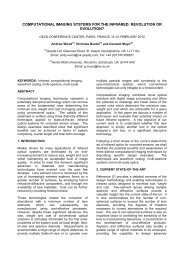
Holographic generation and orbital angular momentum of high ...

INSTITUTE OF PHYSICS PUBLISHINGJOURNAL OF OPTICS B: QUANTUM AND SEMICLASSICAL OPTICSJ. Opt. B: Quantum Semiclass. Opt. 4 (2002) S52–S57 PII: S1464-4266(02)30546-9Holographic generation and orbitalangular momentum of high-orderMathieu beamsSChávez-Cerda 1,4 , M J Padgett 2 , I Allison 2 ,GHCNew 1 ,JCGutiérrez-Vega 3 ,ATO’Neil 2 ,IMacVicar 2 and J Courtial 21 Quantum Optics and Laser Science Group, Imperial College, London SW7 2BW, UK2 Department of Physics and Astronomy, University of Glasgow, Glasgow G12 8QQ, UK3 Instituto Nacional de Astrofisica, Optica y Electrónica, Apartado Postal 51/216,Puebla, Mexico 72000E-mail: j.courtial@physics.gla.ac.ukReceived 6 November 2001, in final form 4 February 2002Published8March2002Onlineatstacks.iop.org/JOptB/4/S52AbstractWe report the first experimental generation of high-order Mathieu beamsand confirm their propagation invariance over a limited range. In ourexperiment we use a computer-generated phase hologram. The peculiarbehaviour of the vortices in Mathieu beams gives rise to questions abouttheir orbital-angular-momentum content, which we calculate by performinga decomposition in terms of Bessel beams.Keywords: Computer-generated holograms, orbital angular momentum oflight, diffraction-free beams1. IntroductionEver since Durnin’s description of Bessel beams [1, 2],diffraction-free light beams, of which Bessel beams were thefirst non-trivial example, have been the subject of intensetheoretical and experimental interest. Potential applicationsof non-diffracting optical and ultrasonic beams range fromlithography [3] through optical communications [4] to medicalimaging [5].The history of diffraction-free beams started with Durnin’srealization that in Whittaker’s solution [6, 7] to the Helmholtzequation,u(x, y, z > 0) = exp(ik z z)∫ 2π0A(φ)× exp(ik r (x cos φ + y sin φ))dφ (1)the intensity |u(x, y, z)| 2 is independent of z, and the beamsit represents are therefore diffraction-free [1]. Durnininvestigated the case A(φ) = const., and found that theresulting field u is given byu(r, z > 0) ∝ exp(ik z z)J 0 (k r r) (2)4 Present address: Instituto Nacional de Astrofisica, Optica y Electrónica,Apartado Postal 51/216, Puebla, Mexico 72000.where J 0 is a Bessel function (of the first kind). Such a beamis known as a zero-order Bessel beam. It was later foundthat functions A(φ) ∝ exp(imφ) lead to higher-order Besselbeams [8], which are of the formu(r,φ,z > 0) ∝ exp(ik z z) exp(imφ) · J m (k r r). (3)Soon after the discovery of Bessel beams as formalsolutions to a differential equation the following intuitiveexplanation was found for the diffraction-free property ofBessel beams [2]. This explanation also provides an elegantinterpretation of the function A(φ).Any light beam can be described as a superposition ofplane waves of the form exp(i(k x x+k y y+k z z)). On propagationover a distance z each plane-wave component suffers anindividual phase shift of k z z. In general, different plane-wavecomponents suffer different phase shifts, so their interferencepattern, i.e. the light beam, changes shape. (This mechanism isthe basis of frequently used beam propagation algorithms; seefor example [9].) However, there are special cases in whichthe plane-wave components always stay in phase, namelywhen the phase shift k z z is the same for every plane-wavecomponent. Such light beams do not change on propagation,not even in scale. (Note that structurally stable beams such1464-4266/02/020052+06$30.00 © 2002 IOP Publishing Ltd Printed in the UK S52

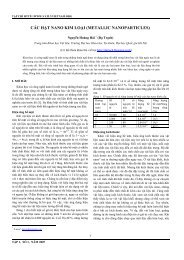
SChávez-Cerda et alA 1Hf 1L 1A 2-2-1f 20L 2+1f 1+2f 2H′zCFigure 3. Schematic of the experiment for the holographicgeneration of higher-order Mathieu beams. The phase hologram His illuminated by a beam truncated by the circular aperture A 1 .Inthe focal plane of lens L 1 the circular aperture A 2 picks out thebright ring of the first diffraction order, which is then turned into adiffraction-free beam by the lens L 2 . The CCD array C allows theintensity cross sections of the resulting beam to be recorded atvarious distances z behind the image of the hologram, H ′ . The focallengths used in our experiment were f 1 = 600 mm andf 2 = 250 mm.(a)(b)-2 -1 0 +1 +2Figure 4. Experimentally recorded intensity cross sections in thefocal plane of a lens behind Mathieu-beam phase holograms undertop-hat illumination for k r = 3 × 10 4 m −1 (recorded behind m = 5and q = 7 hologram, see figure 2) (a) andfork r = 4 × 10 4 m −1(recorded behind m = 5andq = 20 hologram) (b). The diffractionorders are identified at the bottom.z max =rtan θ . (5) allowing the zeroth-order diffracted beam to pass through theaperture A 2 . Comparison with figure 2 confirms that the beamsFigure 5. Intensity cross sections of different experimentallygenerated higher-order Mathieu beams at different distances zbehind the plane H ′ (see figure 3). The three different beamscorrespond to the three holograms shown in figure 2. The arearepresented by each image is approximately 0.5 mm by 0.4 mm.Here r is the radius of the beam in the plane of the aperture (thebase of the cone) and θ is the inclination angle of the beam’splane-wave components with respect to the optical axis. Therelevant aperture in our experiment is the image of A 1 in theplane H ′ , which has a radius of r ≈ 1.6 mm (the radius of A 1is about 3.75 mm, and its image in the plane H ′ is magnifiedby a factor of M =−f 2 /f 1 ≈−0.42). The angle θ can becalculated from the equation tan θ ≈ sin θ = k r /k, whichinour experiment evaluated to θ ≈ 0.55 ◦ and θ ≈ 0.42 ◦ forholograms with k r = 4 × 10 4 m −1 and k r = 3 × 10 4 m −1 ,respectively. (Note that imaging the beam from the plane Hinto the plane H ′ with magnification M changes k r by afactor 1/|M|.) These values lead to respective diffractionfreedistances of r max ≈ 162 mm (for θ ≈ 0.55 ◦ )andr max ≈ 215 mm (θ ≈ 0.42 ◦ ), which are in good agreementwith the distances after which the centre of the beams in ourexperiment became much fainter (figure 5).Figure 6 shows interference patterns between the Mathieubeams and an inclined plane wave, illustrating the phasestructure of the beams. The plane wave was obtained by alsoperfect circle. As this plane also happens to be the front focalplane of lens L 2 , our set-up is essentially of the type shownin figure 1; the first part of the set-up, including illumination,hologram, lens L 1 , and aperture A 2 , is therefore simply a wayof creating, in the front focal plane of lens L 2 , a ring-shapedlight field with the azimuthal field dependence A(φ) that leadsto a Mathieu beam behind the lens.Figure 5 shows intensity cross sections through theMathieu beams produced with the holograms shown in figure 2.It can clearly be seen that the beams are diffraction free onlyover a finite distance, z max , the so-called propagation-invariantregion, behind which the centre of the beam rapidly becomesfainter. This is a well known effect due to the finite size ofthe beam. The slight rotation about the optical axis withinthe propagation-invariant region, which can also be seen infigure 5, has been predicted theoretically very recently [11]and is also due to the beam’s finite size. The distance z maxcan be estimated geometrically to be the length of the conein which all the plane-wave components in the beam intersect(see figure 1), which is given by [1]S54

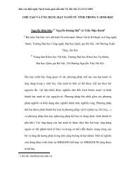
SChávez-Cerda et alm = 6, q = 0m = 6, q = 18m = 6, q = 27m = 6, q = 72|u(x,y)| 2108×3arg(A(φ)) |A(φ)| 2 arg(u(x,y))δl z (φ)|A l | 2~δL z /64200 50 100 150qFigure 10. OAM per photon, δL z , of Mathieu beams with m indicesbetween 0 and 10, plotted as a function of q. Thecurvecorresponding to a specific value of m starts off at q = 0 with avalue δL z (0) = m¯h. The dotted line crosses these curvesapproximately at the critical values q c . The circles mark the casesthat are shown in more detail in figure 9.-10 0 10 -10 0 10 -10 0 10 -10 0 10Figure 9. Examples of Mathieu beams and calculation of theirorbital angular momenta. In the back focal plane of a lens, theMathieu beams described by the functions u(x, y) (shown are theintensity and phase cross sections, |u(x, y)| 2 and arg(u(x, y)))arethin bright rings with an angular amplitude distribution of the formA(φ) (again, the intensity and phase distributions are shown over thefull φ range between 0 and 2π). The local OAM per photon, δl z (φ)(the vertical range corresponds to values between 0 and 20¯h), can becalculated from arg(A(φ)). The power spectra of A(φ), |Ã l | 2 ,arealso the Bessel-beam spectra of the corresponding Mathieu beams.The respective orbital angular momenta per photon, δL z ,are6¯h(q = 0), 4.92¯h (q = 18), 4.40¯h (q = 27) and 6.32¯h (q = 72). In thecase q = 72 numerous additional vortices can be spotted in thebeam’s phase cross section, arg(u(x, y)).Note that regions of zero intensity, such as for examplethe cylindrical surfaces of zero-field amplitude in Besselbeams, do not contribute to δL z —the density of OAM is zerothere.When calculating the OAM content of perfectlydiffraction-free light beams, it is useful to be aware of someof their peculiarities. Most importantly, perfectly diffractionfreelight beams are infinitely wide—this is the reason whyexperimental realizations of diffraction-free beams, whichare always limited by a finite aperture, can only ever beapproximations and do exhibit diffraction effects, such asthe finite range of ‘diffraction-free’ propagation observed insection 2 [2]. Closely related to their infinite width is theinfinite energy content of perfectly diffraction-free light beams.Bessel beams, for example, have approximately the same—finite—amount of energy in each of the concentric bright rings,of which there are infinitely many [1]. As the OAM per photon,δL z , is proportional to the ratio of OAM and energy, perfectlydiffraction-free beams with non-zero values of δL z thereforepossess an infinite OAM.Perhaps the following subtle point merits a briefdiscussion: the OAM flux (equation (8)) was calculated withrespect to the origin. At first this might appear to restrictthe generality of this approach; however, as the OAM of alight beam in the direction of the beam’s propagation direction(more precisely the direction of the momentum vector of theentire beam) is independent of the choice of axis and thereforeintrinsic [21], it does not matter relative to which axis itis calculated, as long as the axis is parallel to the beam’spropagation direction.Numerically, the gradients in equation (7) can beapproximated by finite differences, for example in the form∂u/∂x ≈ (u(x + , y) − u(x − , y))/(2), and theintegration in equation (9) can be replaced by a summationover a discrete number of values. The OAM per photon cantherefore be calculated quite easily from values of u(x, y) at afinite number of points on a beam cross section.It can be shown that in polar coordinates the expressionfor δl z becomesδl z (r,φ)= d(r,φ)dφ· ¯h (10)where (r,φ)is the phase cross section of the light beam. (Forthe local OAM per photon of a light beam with an azimuthalphase dependence of the form (φ) = lφ this gives δl z = l¯heverywhere and therefore δL z = l¯h, as expected [20]. Astheir azimuthal phase term is of the form exp(imφ), Mathieubeams with q = 0 (i.e. Bessel beams) have an azimuthal phasedependence of the form (φ) = mφ and therefore an OAMper photon of δL z = m¯h.) For diffraction-free beams, thisexpression can be evaluated in the far field, where the intensitycross section is simply a bright circle. In terms of the fielddistribution on this circle, A(φ), equation (10) becomesδl z (φ) = d arg(A(φ)) · ¯h. (11)dφFigure 9 shows some examples of intensity and phase crosssections through Mathieu beams, alongside the correspondingfunctions A(φ) and the local OAM per photon, δl z (φ).S56

Note that care has to be taken with 2π phase jumps in thefunction arg(A(φ)).A completely different approach for the calculation of theOAM per photon in a light beam involves a decompositionin terms of beams components with known orbital angularmomenta, like for example Laguerre–Gaussian beams orBessel beams (equation (3)), which have an azimuthal phaseterm of the form exp(ilφ), i.e. an azimuthal phase dependence(φ) = lφ, and therefore an OAM per photon of l¯h. Thesumof the per-photon orbital angular momenta of these individualbeam components, weighted by the corresponding relativeintensities, is the OAM per photon of the beam as a whole.Diffraction-free beams are special in that they can bedecomposed very easily in terms of Bessel beams: a Fouriertransform of the azimuthal amplitude distribution in the farfield (or at the focus of a lens), A(φ), taking into accountthat A(φ) is 2π-periodic, yields the discrete set of Fouriercoefficients à l of the exp(ilφ) components of the beam(equation (47) in [22]). The OAM per photon in the beamis simply∑lδL z =l|à l | 2∑l |à · ¯h. (12)l |2Alongside beam cross sections, u(x, y), azimuthal fielddistributions in the far field, A(φ), and corresponding localorbital angular momenta per photon, figure 9 also shows arepresentation of the Fourier coefficients, à l , for some Mathieubeams.4. Orbital angular momentum of Mathieu beamsIn light beams with a phase structure of the form exp(ilφ), likefor example Bessel beams, the local OAM per photon, δl z ,hasthe constant value l¯h everywhere, which is also the value of thebeam’s OAM per photon, δL z . This is not the case in Mathieubeams, which exhibit a much more complex phase structure.Figure 10 shows plots of δL z as a function of q forMathieu beams with m = 0, 1,...,10; for negative valuesof m, δL z simply changes sign. The curves were obtainedby calculating the m coordinate of the centre of gravity ofthe power spectrum of A(φ), as outlined in section 3. Apartfrom the curve for m = 0, which is zero everywhere, thecurves all start from δL z = m¯h at q = 0 and, as q increases,smoothly decrease, pass through a minimum, and increaseagain, sometimes crossing the curve for a different value of m.For m =±1, the minimum appears to be located at q = 0.The curves are continuous everywhere, including at the criticalvalues q c , where numerous new vortices start to appear in thebeam.5. ConclusionsWe have reported the first experimental generation of higherorderMathieu beams. We show that important properties ofthe holographic method used are illustrated very clearly whenapplied to diffraction-free beams; in particular, the effect ofuniform illumination of the hologram manifests itself in thefar fieldintheformof‘radial harmonics’, i.e. additional ringswhose radius is an integer multiple of the ‘fundamental’ ring.We have also calculated the OAM content of all Mathieu beamswithin a large area of parameter space.AcknowledgmentsGeneration of high-order Mathieu beamsSC-C acknowledges support by the Engineering and PhysicalSciences Research Council (grant no GR/N37117/01). Thiswork was partially supported by Consejo Nacional de Cienciay Tecnologia. MJP and JC acknowledge support from theRoyal Society.References[1] Durnin J 1987 Exact solutions for nondiffracting beams: I.The scalar theory J. Opt. Soc. Am. A 4 651–4[2] DurninJ,MiceliJJJandEberlyJH1987 Diffraction-freebeams Phys.Rev.Lett.58 1499–501[3] Erdélyi M, Horváth Z L, Szabó G, Bor S, Tittel F K,Cavallaro J R and Smayling M C 1997 Generation ofdiffraction-free beams for applications in opticalmicrolithography J. Vac. Sci. Technol. B15 287[4] Lu J-Y and He S 1999 Optical X wave communications Opt.Commun. 161 187–92[5] Lu J-Y and Greenleaf J F 1994 A study of two-dimensionalarray transducers for limited diffraction beams IEEE Trans.Ultrason. Ferroelectr. Freq. Control 41 724–39[6] Whittaker E T 1902 On the partial differential equations ofmathematical physics Math. Ann. 57 333–55[7] Whittaker E T and Watson G N 1927 A Course of ModernAnalysis 4th edn (Cambridge: Cambridge University Press)ch XVIII–XIX[8] Vasara A, Turunen J and Friberg A T 1989 Realization ofgeneral nondiffracting beams with computer-generatedholograms J. Opt. Soc. Am. A 6 1748–54[9] Sziklas E A and Siegman A E 1975 Mode calculation inunstable resonators with flowing saturable gain: 2: FastFourier transform method Appl. Opt. 14 1874–89[10] Gutiérrez-Vega J C, Iturbe-Castillo M D and Chávez-Cerda S2000 Alternative formulation for invariant optical fields:Mathieu beams Opt. Lett. 25 1493–5[11] Chávez-Cerda S, Gutiérrez-Vega J C and New G H C 2001Elliptic vortices of electromagnetic wavefields Opt. Lett. 261803–5[12] Gutiérrez-Vega J C, Rodríguez-Dagnino R andChávez-Cerda S 2002 Attentuation characteristics in confocalannular elliptic waveguides and resonators IEEE Trans.Microwave Theory and Techniques at press[13] McLachlan N W 1951 Theory and Applications of MathieuFunctions (London: Clarendon)[14] Berry M 1981 Singularities in waves and rays Les HouchesLecture Series Session XXXV ed R Balian, M Kléman andJ-P Poirier (Amsterdam: North-Holland) pp 453–543[15] Soskin M S and Vasnetsov M V 2001 Singular optics Prog.Opt. 42 219–76[16] Gutiérrez-Vega J C, Iturbe-Castillo M D, TepichínE,Rodríguez-Dagnino R M, Chávez-Cerda S and New G H C2001 Experimental demonstration of optical Mathieu beamsOpt. Commun. 195 35–40[17] Turunen J, Vasara A and Friberg A T 1988 Holographicgeneration of diffraction-free beams Appl. Opt. 27 3959–62[18] O’Neil A T 2001 PhD Thesis University of St Andrews[19] Bjelkhagen H I 1993 Silver-Halide Recording Materials(Berlin: Springer) ch 5[20] Allen L, Beijersbergen M W, Spreeuw R J C and WoerdmanJ P 1992 Orbital angular momentum of light and thetransformation of Laguerre–Gaussian modes Phys. Rev. A45 8185–9[21] Berry M 1998 Paraxial beams of spinning light SingularOptics ed M S Soskin Proc. SPIE 3487 (SPIE Int. Soc. Opt.Engng.) (Bellingham, Washington, USA) pp 1–5[22] Siegman A E 1986 Lasers (Mill Valley, CA: UniversityScience Books)S57