Holographic generation and orbital angular momentum of high ...

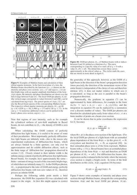
SChávez-Cerda et alm = 6, q = 0m = 6, q = 18m = 6, q = 27m = 6, q = 72|u(x,y)| 2108×3arg(A(φ)) |A(φ)| 2 arg(u(x,y))δl z (φ)|A l | 2~δL z /64200 50 100 150qFigure 10. OAM per photon, δL z , of Mathieu beams with m indicesbetween 0 and 10, plotted as a function of q. Thecurvecorresponding to a specific value of m starts off at q = 0 with avalue δL z (0) = m¯h. The dotted line crosses these curvesapproximately at the critical values q c . The circles mark the casesthat are shown in more detail in figure 9.-10 0 10 -10 0 10 -10 0 10 -10 0 10Figure 9. Examples of Mathieu beams and calculation of theirorbital angular momenta. In the back focal plane of a lens, theMathieu beams described by the functions u(x, y) (shown are theintensity and phase cross sections, |u(x, y)| 2 and arg(u(x, y)))arethin bright rings with an angular amplitude distribution of the formA(φ) (again, the intensity and phase distributions are shown over thefull φ range between 0 and 2π). The local OAM per photon, δl z (φ)(the vertical range corresponds to values between 0 and 20¯h), can becalculated from arg(A(φ)). The power spectra of A(φ), |Ã l | 2 ,arealso the Bessel-beam spectra of the corresponding Mathieu beams.The respective orbital angular momenta per photon, δL z ,are6¯h(q = 0), 4.92¯h (q = 18), 4.40¯h (q = 27) and 6.32¯h (q = 72). In thecase q = 72 numerous additional vortices can be spotted in thebeam’s phase cross section, arg(u(x, y)).Note that regions of zero intensity, such as for examplethe cylindrical surfaces of zero-field amplitude in Besselbeams, do not contribute to δL z —the density of OAM is zerothere.When calculating the OAM content of perfectlydiffraction-free light beams, it is useful to be aware of someof their peculiarities. Most importantly, perfectly diffractionfreelight beams are infinitely wide—this is the reason whyexperimental realizations of diffraction-free beams, whichare always limited by a finite aperture, can only ever beapproximations and do exhibit diffraction effects, such asthe finite range of ‘diffraction-free’ propagation observed insection 2 [2]. Closely related to their infinite width is theinfinite energy content of perfectly diffraction-free light beams.Bessel beams, for example, have approximately the same—finite—amount of energy in each of the concentric bright rings,of which there are infinitely many [1]. As the OAM per photon,δL z , is proportional to the ratio of OAM and energy, perfectlydiffraction-free beams with non-zero values of δL z thereforepossess an infinite OAM.Perhaps the following subtle point merits a briefdiscussion: the OAM flux (equation (8)) was calculated withrespect to the origin. At first this might appear to restrictthe generality of this approach; however, as the OAM of alight beam in the direction of the beam’s propagation direction(more precisely the direction of the momentum vector of theentire beam) is independent of the choice of axis and thereforeintrinsic [21], it does not matter relative to which axis itis calculated, as long as the axis is parallel to the beam’spropagation direction.Numerically, the gradients in equation (7) can beapproximated by finite differences, for example in the form∂u/∂x ≈ (u(x + , y) − u(x − , y))/(2), and theintegration in equation (9) can be replaced by a summationover a discrete number of values. The OAM per photon cantherefore be calculated quite easily from values of u(x, y) at afinite number of points on a beam cross section.It can be shown that in polar coordinates the expressionfor δl z becomesδl z (r,φ)= d(r,φ)dφ· ¯h (10)where (r,φ)is the phase cross section of the light beam. (Forthe local OAM per photon of a light beam with an azimuthalphase dependence of the form (φ) = lφ this gives δl z = l¯heverywhere and therefore δL z = l¯h, as expected [20]. Astheir azimuthal phase term is of the form exp(imφ), Mathieubeams with q = 0 (i.e. Bessel beams) have an azimuthal phasedependence of the form (φ) = mφ and therefore an OAMper photon of δL z = m¯h.) For diffraction-free beams, thisexpression can be evaluated in the far field, where the intensitycross section is simply a bright circle. In terms of the fielddistribution on this circle, A(φ), equation (10) becomesδl z (φ) = d arg(A(φ)) · ¯h. (11)dφFigure 9 shows some examples of intensity and phase crosssections through Mathieu beams, alongside the correspondingfunctions A(φ) and the local OAM per photon, δl z (φ).S56