6. Linear Differential Equations of the Second Order--general ...

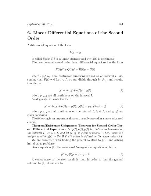
September 26, 2012 6-16. Linear Differential Equations of the SecondOrderA differential equation of the formL(y) = gis called linear if L is a linear operator and g = g(t) is continuous.The most general second order linear differential equations has the formP (t)y ′′ + Q(t)y ′ + R(t)y = G(t)where P, Q, R, G are continuous functions defined on an interval I. Assumingthat P (t) ≠ 0 for t ∈ I, we can divide through by P (t) and rewritethis d.e. asy ′′ + p(t)y ′ + q(t)y = g(t) (1)where p, q, g are all continuous on the interval I.Analogously, we write the IVPy ′′ + p(t)y ′ + q(t)y = g(t), y(t 0 ) = y 0 , y ′ (t 0 ) = y ′ 0 (2)where p, q, g are all continuous on the interval I, t 0 ∈ I, and y 0 , y ′ 0 aregiven constants.The following is an important theorem, usually proved in a more advancedcourse.Theorem(Existence-Uniqueness Theorem for Second Order LinearDifferential Equations). Let p(t), q(t), g(t) be continuous functions onthe interval I, let t 0 ∈ I, and let y 0 , y ′ 0 be given constants. Then, there is aunique solution y(t) to the IVP (2) which is defined on the whole interval I.We are concerned with finding the general solution to (1) , and solvinginitial value problems.Given equation (1), the associated homogeneous equation is the d.e.y ′′ + p(t)y ′ + q(t)y = 0 (3)A consequence of the next result is that, in order to find the generalsolution to (1), it suffices to

September 26, 2012 6-2and1. find the general solution y h to (3), (4)2. find a particular solution y p to (1). (5)The general solution to (1) is then obtained asy = y h + y p .Theorem. Let y p (t) be a particular solution to (1). Then, every solutiony(t) to (1) can be expressed as y(t) = y 1 (t)+y p (t) where y 1 (t) is a solution to(3). Conversely, for any solution y 1 (t) of (3), the function y(t) = y 1 (t)+y p (t)is a solution to (1).Proof.Let y p (t) be a particular solution to (1), and let y(t) be any other solutionto (1). Consider the functiony 1 (t) = y(t) − y p (t).We clearly have y(t) = y 1 (t) + y p (t). Let us verify thatBy linearity,y 1 is a solution to (3). (6)L(y 1 ) = L(y(t) − y p (t)) = L(y(t)) − L(y p (t)) = g(t) − g(t) = 0,which verifies (6).Converse:Let y 1 (t) be solution to (3), and let y(t) = y 1 (t) + y p (t).Then,L(y) = L(y 1 + y p ) = L(y 1 ) + L(y p ) = 0 + g(t) = g(t),so, y is a solution to (1). QED.In view of the preceding theorem, we need to study methods to handlethe problems (4) and (5).We begin with (4).

September 26, 2012 6-3It turns out that to solve this problem, it suffices to find two solutionswhich satisfy a condition called linear independence.Defintion. A pair of functions y 1 (t), y 2 (t) defined on an interval I iscalled a linearly independent pair of functions (on I) if whenever there areconstants c 1 , c 2 such thatc 1 y 1 (t) + c 2 y 2 (t) = 0, ∀t ∈ I,we have c 1 = c 2 = 0.This means that if c 1 y 1 + c 2 y 2 is the zero function on I, it follows thatc 1 = c 2 = 0.We state some theorems which allow us to find the general solution tosecond order homogeneous linear differential equations.We will justify the theorems later.Theorem. Let y 1 (t), y 2 (t) be a linearly independent pair of solutions to(3) on the interval I. Then, the general solution to (3) has the formy(t) = c 1 y 1 (t) + c 2 y 2 (t).Definition. A 2 × 2 matrix is an array of the formA =( )a11 a 12a 21 a 22where the a ij are real or complex numbers. When they are real, we saythat A is a real matrix.Definition. The determinant det(A) of the 2×2 matrix A is the numberdet(A) = a 11 a 22 − a 12 a 21 .Definition. The Wronskian at t 0 of the two functions y 1 , y 2 is thedeterminant( )y1 (tW (y 1 , y 2 )(t 0 ) = det 0 ) y 2 (t 0 )y 1(t ′ 0 ) y 2(t ′ 0 )We also call the function W (y 1 , y 2 )(t) the Wronksian or Wronskian functionof y 1 and y 2 .

September 26, 2012 6-4Theorem(Abel). Two solutions y 1 , y 2 of the the equation (3) arelinearly independent on I if and only if W (y 1 , y 2 )(t) ≠ 0 for some (or any)t ∈ I.Proof. We will show that W = W (t) satisfies the differential equationW (t) ′ = −p(t)W (t) (7)for t ∈ I.Once this is done, let t 0 and t 1 be two points in I.Then,W ′W = −p(t)d(log(W (t))dt= −p(t)log(W (t 1 )) − log(W (t 0 )) =W (t 1 )W (t 0 ) = exp( ∫ t1W (t 1 ) = W (t 0 )exp(t 0∫ t1∫ t1t 0−p(s)ds)t 0−p(s)ds−p(s)ds)Since the exponential term is never zero, we see that W (t 1 ) = 0 if andonly if W (t 0 ) = 0.Now, we turn to the proof of (7).We haveSo,W = y 1 y ′ 2 − y 2 y ′ 1.W ′ = y 1y ′ 2 ′ + y 1 y 2 ′′ − y 2y ′ 1 ′ − y 2 y 1′′= y 1 y 2 ′′ − y 2 y 1′′= y 1 (−py 2 ′ − qy 2 ) − y 2 (−py 1 ′ − qy 1 )= −p(y 1 y ′ 2 − y 2 y ′ 1)= −pW

September 26, 2012 6-5as required. QED.Second Order Linear Homogeneous Differential Equations withConstant Coefficients:These have the formwhere a, b, c are constants and a ≠ 0.Let us first try to find a solution of the formwhere r is a constant.Differentiating, we getay ′′ + by ′ + cy = 0 (8)y = e rt (9)ay ′′ + by ′ + cy = ar 2 e rt + bre rt + ce rt = 0= (ar 2 + br + c)e rt = 0Since e rt is never zero, the only way we could possibly get a solution ofthe form (9) is for r to be a root of the polynomialρ(r) = ar 2 + br + c.This last polynomial is called the characteristic polynomial of the d.e.(8), and the equationρ(r) = ar 2 + br + c = 0 (10)is called the characteristic equation of (8).Proceding in the reverse order, we also see that if r 1 is a root of thecharacteristic equation, then, indeed, y(t) = e r 1t is a solution of (8).Also, if the characteristic equation (10) has two distinct real roots, r 1 , r 2 ,then we get two solutions of the formy 1 (t) = e r 1t , y 2 (t) = e r 2t .Note that this occurs if and only if b 2 − 4ac > 0.We label the roots r 1 , r 2 of ρ(r) so that r 1 > r 2 .Thus, from the quadratic formula, we have

September 26, 2012 6-6r 1 = −b + √ b 2 − 4ac2a, r 2 = −b − √ b 2 − 4ac.2aWe will say that y 1 (t) = e r 1t is the first fundamental solution to (8), andy 2 (t) = e r 2t is the second fundamental solution to (8).Let us see that these turn out to be linearly independent solutions.We compute the Wronskian at t = 0.(y1 (0) yW (y 1 , y 2 )(t) = det2 (0)y 1(0) ′ y 2(0)′( )1 1= detr 1 r 2= r 2 − r 1≠ 0.)Since this non-zero at t = 0 it is non-zero everywhere, so we do havelinearly independent solutions.Hence, the general solution in the case of real distinct roots r 1 , r 2 of (10)isExamples:1. y ′′ − 3y ′ − 4y = 0.Find the roots of r 2 − 3r − 4.y(t) = c 1 e r 1t + c 2 e r 2t .Factoring the polynomial, we getSo, the roots are r 1 = 4, r 2 = −1.r 2 − 3r − 4 = (r − 4)(r + 1).General Solution: y = c 1 e 4t + c 2 e −t .Writing y 1 (t), y 2 (t) for the first and second fundamental solutions, wehave

September 26, 2012 6-7and2. y ′′ + 3y ′ + y = 0y 1 (t) = e 4t ,y 2 (t) = e −t .Characteristic equation: r 2 + 3r + 1 = 0.Use the quadratic formula:So, general solution:r = −3 ± √ 5.2y(t) = c 1 e ( −3+√ 52 )t + c 2 e ( −3−√ 52 )t ,and the first and second fundamental solutions y 1 (t), y 2 (t), respectively,arey 1 (t) = e ( −3+√ 52 )ty 2 (t) = e ( −3−√ 52 )tNow, we know that, given a second degree polynomial ρ(r), we have threepossibilities for its roots r 1 , r 2 .Case 1. r 1 ≠ r 2 and both are realCase 2. r 1 = r 2 ,Case 3. r 1 = α + βi, r 2 = α − βi where i = √ −1.

September 26, 2012 6-8So, finding the general solution to a homogeneous second order linear d.e.with constant coefficients, also involves those three cases.We have already dealt with Case 1.Case 2: r 1 = r 2 . That is, ρ(r) = a(r − r 1 ) 2 .Here we already have one non-zero solution y 1 (t) = e r 1t .We claim that the function y 2 (t) = te r 1t is a second linearly independentsolution.In proceding to verifty this, it will be useful to recall the formula for thesecond derivative of a product.(fg) ′′ = f ′′ g + 2f ′ g ′ + fg ′′ .Now, let us verify that y 2 is a solution.Note that, since, r 1 is a root of multiplicity two, we haveWe havear 2 1 + br 1 + c = 0, and 2ar 1 + b = 0.ay ′′2 + by ′ 2 + cy 2 = a(2r 1 e r 1t + tr 2 1e r 1t ) + b(e r 1t + tr 1 e r 1t ) + cte r 1t= (a2r 1 + b)e r 1t + (ar 2 1 + br 1 + c)te r 1t= 0e r 1t + 0te r 1t = 0.Hence, y 2 is a solution.Now, let us verify that the pair y 1 (t), y 2 (t) is a linearly independent pair.We compute the Wronskian:( )y1 yW (y 1 , y 2 ) = det2y 1 ′ y 2′ (er 1 tte= detr 1tr 1 e r 1te r1t + tr 1 e r 1t= e 2r1t + tr 1 e 2r1t − tr 1 e 2r 1t= e 2r 1t ≠ 0.)Hence, the general solution is:y(t) = c 1 e r 1t + c 2 te r 1t .

September 26, 2012 6-9In Case 2, we define the first and second fundamental solutions y 1 (t), y 2 (t),respectively, byfirst fundamental solution: y 1 (t) = e r 1tsecond fundamental solution: y 2 (t) = te r 1tCase 3: r 1 = α + βi with β ≠ 0.Here we will make use of complex variables.Recall the formulae α+βi = e α (cos(β) + i sin(β)).We first verify that the complex valued functiony(t) = e (α+βi)tis a solution to our d.e. It turns out that the real and imaginary parts ofthis complex solution give linearly independent solutions to the d.e.What are these real and imaginary parts:So, the real part isand the imaginary part isHence, the general solution ise (α+βi)t = e αt (cos(βt) + i sin(βt)) (11)e αt cos(βt)e αt sin(βt).y(t) = e αt (c 1 cos(βt) + c 2 sin(βt)).In the case of complex roots, we define the first and second fundamentalsolutions to (8).First fundamental solution: y 1 (t) = e αt cos(βt)Second fundamental solution: y 2 (t) = e αt sin(βt)Examples:

September 26, 2012 6-101. Find the general solution and the first and second fundamental solutionsy 1 (t), y 2 (t) toy ′′ + 6y ′ + 9y = 0.Solution: r 2 + 6r + 9 = (r + 3) 2 , so the general solution is:y(t) = c 1 e −3t + c 2 te −3t .The first and second fundamental solutions are:y 1 (t) = e −3t , y 2 (t) = te −3t2. Find the general solution and first and second fundamental solutionstoy ′′ + y ′ + 3y = 0.Solution:Step 1: Roots of characteristic equation.r 2 + r + 3 = 0.General Solution:y(t) = e − t 2 (c1 cos(r = −1 ± √ 1 − 122= −1√11i2 ± 2First and second fundamental solutions:√11t√11t2 ) + c 2 sin(2 )).y 1 (t) = e − t 2 cos(√11t2 ), y 2(t) = e − t 2 sin(√11t2 )

September 26, 2012 6-111 SummaryConsider the differential equationay ′′ + by ′ + cy = 0where a, b, c are real constants and a ≠ 0.Let q(r) = ar 2 + br + c = 0 be the characteristic equation.Let r 1 = −b+√ b 2 −4ac, r2a 2 = −b−√ b 2 −4acbe the roots of q(r) = 0.2aCase 1: r 1 ≠ r 2 , both real, r 1 > r 2 ,General Solution:y(t) = c 1 e r 1t + c 2 e r 2tFirst and second fundamental solutions:Case 2: r 1 = r 2 ≠ 0General Solution:y 1 (t) = e r 1t , y 2 (t) = e r 2ty(t) = c 1 e r 1t + c 2 te r 1tFirst and second fundamental solutions:y 1 (t) = e r 1t , y 2 (t) = te r 2tCase 3: r 1 = α + βi, r 2 = α − βi, complex with β ≠ 0General Solution:y(t) = e αt (c 1 cos(βt) + c 2 sin(βt))First and second fundamental solutions:y 1 (t) = e αt cos(βt), y 2 (t) = e αt sin(βt)