Linear Algebra - Capitol College Faculty Pages

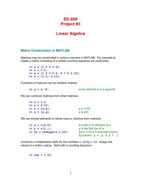
EE-600Project #3Linear AlgebraMatrix Construction in MATLABMatrices may be constructed in various manners in MATLAB. For example tocreate a matrix consisting of a simple counting sequence we could enter>> x = [1 2 3 4 5];>> x = 1:5;>> x = [1 2 3 4 5; 6 7 8 9 10];>> x = [1:5; 6:10];Functions of matrices can be similarly entered>> y = x.^2; every element in x is squaredWe can construct matrices from other matrices:>> x = 1:5;>> y = 6:10;>> z = [x,y]; z is 1x10>> z = [x;y]; z is 2x5We can extract elements or whole rows or columns from matrices:>> x = z(2,2); x is the (2,2) element of z>> y = z(1,:); y is the first row of z>> zz = reshape(z,1,10); zz is 1x10 z is scanned columnby column: z = [1 6 2 7 …]Construct a multiplication table for the numbers 1-10 by 1-10. Assign thevalues to a matrix table. Start with a counting sequence>> row = 1:10;1

Assign multiples of this row to rows of table. The same multiplication table canbe made using the kron() function in two lines—show howGraphics with MatricesThe most basic kind of plot in MATLAB is with two one-dimensional matrices xand y:>> plot (x, y);The plot is a solid line by default. If you wish to specify another line type, youmay specify a third argument. For example>> plot (x, y, ':');plots a dotted line.. Suppose you wished to plot the poles of a transfer functionwhose denominator is a.>> p = roots(a);>> plot (real(p), imag(p), 'x');Write some MATLAB code that will take a transfer function H find the numeratorand denominator, find the zeroes and the poles and plot them appropriately (witha ‘o’ for zeroes). Label the axes Re{s} and Im{s} using the MATLABfunctions xlabel()and ylabel(). To get the numerator and denominator fora transfer function, use tfdata(), e.g.,>> H = tf(num, den);>> [num, den] = tfdata(H,'v');Sometimes, the x and y arguments in the plot do not have the same dimension.When y has two dimensions, multiple plots are made, column-by-column. The xspecifies the common abscissa. The hard part in these plots is specifying the yarray. This is where the kron() function can be used: it makes matrices out ofmatrices.Create a plot of the first three terms of the Fourier series for a square wave usinga single plot() command. Create the two-dimensional matrix y using thekron() function. The kron() function will use>> t = 0:0.01:1;>> n = [1 3 5];The result should look like Figure 1.2

10.80.60.40.20-0.2-0.4-0.6-0.8-10 0.1 0.2 0.3 0.4 0.5 0.6 0.7 0.8 0.9 1Figure 1. Output of plot(t,y) for the first three harmonics of the Fourier seriesof a square wave.Matrix ManipulationThere seems to be no end to the number of matrix functions and operations inMATLAB.Matrix InversesMatrix inverses may be found by the method of cofactors: first replace eachelement by its cofactor, i.e., the determinant of the matrix found from the otherrows and columns. Write a MATLAB routine (function) to find the cofactor ofelement i,j of a matrix A. You may use the MATLAB det() function. Use thiscofactor routine to find the inverse of a matrix A.Eigenvalues and EigenvectorsCreate a matrixA=[ −5 1−6 0 ]3

and find the eigenvalues and eigenvectors of A first by hand and then check yourwork by using the MATLAB command>> [P,D] = eig(A)The eigenvectors that you will get by hand should be proportional to theeigenvectors produced by MATLAB. Using MATLAB, verify thatD=P −1 AP.Create a matrix whose eigenvalues are –5 and –10. The matrix cannot simply bea diagonal matrix with elements –5 and –10: use the D=P -1 AP to find the matrix.Check your answer using the eig() function. (Hint: it does not matter what theeigenvectors are so long as they are independent.)Linear TransformationsSuppose we wished to “rotate” a set of points plotted on a Cartesian plane. Forexample consider the points (1,1), (2,2), (3,3), (4,4), (5,5) plotted in Figure 2. Wecan plot these points by creating two matries x, y and plotting them:>> x = 1:5;>> y = 1;5;>> plot(x,y);Each point can then be transformed using a linear transformation:[ x ]newy = cosθ −sin θnew[ sin θ] y .oldcosθ ][ x oldWhen we plot the transformed points for θ=-45°, we get the plot in Figure 3.Perform this transformation: create a composite point matrix point consisting oftwo rows: one for the (five) x-values and one for the y-values. Transform thiscomposite matrix using the rotation matrix[cosθ −sin θsin θ cosθ ]4

into a new matrix newpoint. Extract the new x-values and y-values from thenew matrix into two new matrices: xnew and ynew, and plot them. Your plotshould resemble Figure 3.5

108642y0-2-4-6-8-10-10 -8 -6 -4 -2 0 2 4 6 8 10xFigure 2. Output of plot(x,y) for five points.108642y0-2-4-6-8-10-10 -8 -6 -4 -2 0 2 4 6 8 10xFigure 3. Output of plot(xnew,ynew) for five points.6