3.0 visual feature extraction and classification - DSpace@UM

Chapter 3The higher level features can be divided into two distinguished categories as syntacticfeatures and semantic features (Konstantinou et al., 2009; Mittal, 2006). Syntacticfeatures are derived from direct operations of pixel level data of an image or a video; foran example, object boundaries or histogram of a frame. On the other hand, semanticfeatures are derived through a number of process operations and mappings; for example,listing of sea area, sky area and mountains. The semantic level of video sequencecontains levels of abstraction, which depends on sequence of frames, motions, objects,brightness, surrounding, and the relationships with other video attributes such as audio,prior scenes and video text. Using high level semantic features for video retrieval allowspeople to perform search at the semantic level, which is more intuitive. High levelsemantic features can be obtained by integrating additional knowledge of a specificdomain with low level features (Zheng et al., 2006).In recent past, researchers have focused on the use of internal features of images andvideos computed in an automated or semi-automated way (Lew et al., 2006). Mostanalysis use statistics and probability approaches which can be approximately correlatedto the content features (Aghbari & Makinouchi, 2003; Datta et al., 2005; Fasel, 2006;Heller & Ghahramani, 2006). These approaches provide information without costlyhuman interaction. Researchers are commonly focusing on the syntactic features ratherthan the semantic features of visual contents (Israël, Broek, Putten, & Uyl, 2004). Somecontent-based retrieval systems that operate at semantic level would identify motionfeatures as the key element besides other features such as colour, objects and texture,because motion (either camera motion or shot editing) adds additional meaning to thecontent.The performance of high level feature extractions is currently not adequate and greatlyrestricts the search performance (Zheng et al., 2006). There is a need to further improve40

Chapter 3the performance of high level feature extraction. Meanwhile researches should considerthe reliabilities of semantic feature detectors more carefully as it is the key to the highlevel feature extraction. One heuristic in the selection process is to have applicationspecificfeature sets, and this has given some positive results in the retrieval ofsemantic-sensitive data (Datta et al., 2005).3.3. Use of Colour Features in Content RetrievalColour is the most common syntactic feature for most researches in image and videocontent analysis. In use of colours, different colour representations have been used bydifferent experiments done in different scales. The popular colour modes are RGB (Red,Green, Blue), HSV/I (Hue, Saturation, Value/Intensity) and Gray levels. Colour featurespresent the amount and distribution of colors in an image. The rationale for thesefeatures is that images of similar objects or concepts usually have similar colours(Pakkanen, 2006). In querying a colour image by using an image retrieval system, ascan is operated for the similar colour distribution in the image database to match thequery. In the case of query by example, the algorithms’ task is to find the similar colourdistribution according to the example image.A pixel can be represented by different colour attributes that are described by differentcolour modes and stored in different data structures. All visual features are composed ofmany colour attributes. To describe a pixel, RGB, HSV, Gray and CIE-LUV (CIE Lab)colour models are common. Some image processing techniques give different results fordifferent models. The digital video pixels are products of a raster scanning or directresults from Charge Couple Device (CCD)/Exmore arrays in digital cameras (Y. Wang,Ostermann, & Zhang, 2002). According to the International Telecommunications Union- Radio Sector (ITU-R) BT. 601 standards, digital video has to be maintained with 4:3or 16:9 aspect ratio (Image Width: Image Height) (Y. Wang et al., 2002). Further,41

Chapter 3recommendation given for a digital colour coordinate is YCbCr (one luminance and twochrominance components). The Y, Cb, and Cr components are scaled and shiftedversions of the analog Y, U, and V components, whereby the scaling and shiftingoperations are introduced so that the resulting components take value in the range of(0,255). The choice of colour models is a matter of the conversion of a model to anotherand it is an easy process.3.4. Syntactic Visual FeaturesSyntactic visual features derived from colour data of video frames are the key to derivesemantic concepts in videos. There are different syntactic visual features commonlyused in many applications.3.4.1. Colour HistogramsColour histograms are often used for matching process (Lew, 2000). Although colourhistograms which are often used for matching processes are useful as they are relativelyinsensitive to position and orientation changes, they do not capture spatial relationshipof colour regions and thus they have limited discriminating power (Lavee, Khan, &Thuraisingham, 2007; Lew, 2000; Maron & Ratan, 1998; Nicu Sebe & Lew, 2001).More recently, researchers have introduced spatial histogram to integrate spatialdescription into histogram based techniques. MPEG-7 visual description guidelines alsomention about spatial histograms, but they do not describe micro level patterndistributions (MPEG-7, 2004).In the calculation for the most relevant match of the colour distribution, the probabilisticand statistical techniques are commonly used with techniques based on average colourvalues, standard deviations and 3D histogram comparisons which are computationallyexpensive. In some studies, 3D histograms are used in colour feature comparison with42

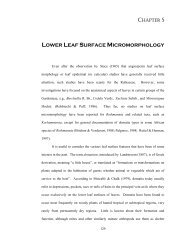
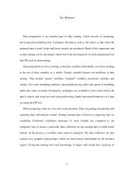
Chapter 3HSV components (Heller & Ghahramani, 2006). If the images originate from diversesources then parameters such as quality, resolution and colour depth would likelyvaried. This in turn causes variations in the extracted colour and texture features (Dattaet al., 2005). This is true for video frames as well.Commonly histograms lack in terms of describing micro level or texel level informationand are also not accompanied with spatial information. Therefore they give pooraccuracy in concept detection. Most colour histograms are used with 125 bins (S. Gao,Zhu, & Sun, 2007). However this number of dimensions also negatively affects thecomputations that take place in the classification process. The HSV types of histogramsrequire colour conversions in addition to RGB histograms. The L*a*b histogramcontains 96 dimensions (Giang & Worring, 2008). Histograms are always likely to becombined with multiple features for accurate concept detection, such as texture featuresand shape features which cause increase in computational costs. Figure 3.1 representscolour histograms with different channels including RGB.Figure 3.1: Colour Histogram Representation of an Image3.4.2. Texture Features in Content RetrievalIn most applications, colour feature has been used to identify different object categories,but colour feature methods tend to produce false positives (Mäenpää, Viertola, &43

Chapter 3Pietikäinen, 2004). The visuals that contained similar colour composition can result infalse positives. Texture plays a very important role in visual perception and objectidentities (Ardizzone, Capra, & La Cascia, 2000; Mäenpää et al., 2004). Texturepatterns distinguish structural arrangement of surfaces from the surroundingenvironment; therefore texture is a natural property of all object surfaces. In usingtextures, both colour and geometrical distribution features give improvement in results(Heller & Ghahramani, 2006; Nicu Sebe & Lew, 2001). The analysis and categorizationof the textures are very crucial. Textures can be classified by using different propertiessuch as coarseness, dominant colour, roughness, colour gradients and periodicalpatterns.In video visuals, texture features available on objects can be used to classify or identifyobjects in scenes. It is difficult to identify and fully understand how human visionsystem segment textures on objects. Some studies have used a mixture of texturefeatures such as Tamura & Gabor texture features in visual content retrievals (Heller &Ghahramani, 2006). According to Tamura et al. (1978), texture features areapproximated in computational form into six basic features, namely, coarseness,contrast, directionality, line-likeness, regularity, and roughness with the help of humanlevel of perception. In addition, Simultaneous Auto-Regressive (SAR) orientation,Gabor and wavelet-transform are also used to describe texture (Ardizzone et al., 2000;Heller & Ghahramani, 2006).‘Textons’ which refer to a set of representative classes of image patches that suffice tocharacterize an image object or texture are typically extracted densely, representingsmall and relatively generic image micro-structures such as blobs, bars and corners(Jurie & Triggs, 2005; Leung & Malik, 2001). Texton representation can be consideredas a form of data compression, but it is not the only way for compressing data (Leung &44

Chapter 3Malik, 2001). Texture can be characterized by a spatial repetition of finite textureelements or 2D (two dimensional) patterns, called texels in an image area occupied by atexture (Todorovic & Ahuja, 2009). Texel which is also known as texture element cancontain several pixels in a 2D array. Normally texels in natural scenes are not identical,and their spatial repetition is not strictly periodic. Instead, texels are only statisticallysimilar to one another, and their placement along a surface is only statistically uniform.Texels are also not homogenous-intensity regions, but may contain hierarchicallyembedded structures. Therefore, the study by Todorovic and Ahuja (2009) havecharacterized an image texture by a probability density function governing the (natural)statistical variations of the following texel properties: (1) geometric and photometric –referred to as intrinsic properties (for example colour, area, shape); (2) structural; and(3) relative orientations and displacements of texels – referred to as placement.Wavelet textures, Gabor textures, and Wiccest textures are dominantly used in videovisual description (Ardizzone et al., 2000; Giang & Worring, 2008; Heller &Ghahramani, 2006; Zheng et al., 2006). Gabor filter (or Gabor wavelet) is widelyadopted to extract texture features from images in image retrieval, and has been shownto be very efficient (Ardizzone et al., 2000; Giang & Worring, 2008; Heller &Ghahramani, 2006). Image retrieval using Gabor features outperforms the usage ofPyramid-structured wavelet transform (PWT) features, tree-structured wavelettransform (TWT) features and multi-resolution simultaneous autoregressive model(MR-SAR) features (Ro, Kim, Kang, Manjunath, & Kim, 2001).Natural sceneries can be effectively described using colour and spatial properties(Maron & Ratan, 1998). The QBIC and VIRAGE systems use colour, structuralproperties and combined with textures in their image query systems (IBM-Corporation,2003; Maron & Ratan, 1998; Virage, 2009). The texture can be static or dynamic.45

Chapter 3Ardizzone et al. (2000) used textures evolving over time, called temporal textures. Thesmoke flowing or wavy water of a river are good examples of temporal textures.Some studies have used the mixture of texture features such as Tamura & Gaborfeatures and Wiccest features, which extend texture properties with colour invarianceand natural image statistics (Heller & Ghahramani, 2006; Snoek et al., 2005). In manysituations, texture features accompanied with colour features enlarge the feature spaceand computational costs, for example the Wiccest feature used in Snoek et al. (2005)contains 108 dimensions (Giang & Worring, 2008; Snoek et al., 2005). Highdimensional texture features increase the computational cost of distance measures use inclassification.3.4.3. Wavelets in Content DescriptionImages and video content are presented in multi resolution environment. In additiondifferent areas and objects in visuals are represented in different scales and resolutions.In this context, description of visual regions by using colour intensity requires multilevel resolution analysis. Consistent resolution within visual regions cannot be expected.Therefore, in processing visuals with multilevel resolutions, the wavelet transformationis widely used. The wavelet representation of images provides information about thevariations in different scales. According to Sebe & Lew (2001), the Haar waveletcomparison method is lagging behind as a salient point extraction due to its nonoverlappingwavelets at a given scale and increase of computations related to spatialsupport.3.4.4. Shape DescriptorsShape is also used as a key attribute of segmented image regions, and its efficient androbust representation plays an important role in some retrieval systems. Shape similarity46

Chapter 3matching is one of the methods that can be used to reduce irrelevant colour features.Datta et al. (2005) describe some performance problems of computation of shapesimilarity matching with geometrical invariance of transformation. In shape matching,dynamic geometrical transformation comparison is a required key feature. In clusteringof shapes in frames, different methods such as colour or spectral clustering, textureclustering and edge clustering are used. For characterizing shapes within images,reliable segmentation is critical, without which the shape estimations are largelymeaningless and the general problem of semantic visual concept segmentation in thecontext of human perception is far from being solved (Datta et al., 2005). Regionclustering is an important step for a successful visual understanding with shapesimilarity matching. Some issues plaguing current shape matching techniques areefficiency consideration, reliability of good segmentation, and a robust and acceptablebenchmark for assessment of the shape matching (Datta et al., 2005).Most visual features are task dependant, particularly shape features. Using shapefeatures to detect circles with constraints in their spatial relations to find cars may givesatisfying results, but may completely fail when applied in searching for flowerbeds(Giang & Worring, 2008). Shape clustering that includes spectral, texture, and edgeclustering can increase computational cost and reduce speed (Datta et al., 2005).3.4.5. Salient and Local Features based MethodsIn video and image retrieval, the use of interest parts of images allows an image andvideo index to represent local properties. There are methods experimented on salientpoint extraction algorithms by extracting colour and texture information in the locationsgiven by these salient points. These methods have shown improved results in terms ofretrieval accuracy, computational complexity, and storage space of feature vectors ascompared to the global feature approaches (Mikolajczyk, Leibe, & Schiele, 2005; Nicu47

Chapter 3Sebe & Lew, 2001). These methods give an improvement over global feature basedretrieval by using feature vector based content retrieval which targets only the relevantpoints in the visual area. In video frame area, different parts are available with differentfeatures. When dealing with global features, video description is extracted by analyzingthe whole frame, and this leads to complication in distinguishing relevant informationfrom irrelevant ones.During early period of using salient feature method, it is applied with corner detectors toobtain the corner points of images (Bay, Ess, Tuytelaars, & Gool, 2008; Mikolajczyk etal., 2005; Nicu Sebe & Lew, 2001). However, this approach failed due to the inability toprovide powerful description of images based on corner points, which may not be theattractive part of an image. Only a small part of an image can be described by corners ascorners tend to be gathered at small area. The Harris corner detector is one of thepopular detectors used for identifying corners as it has strong invariance property inrotation, scale, illumination variation and image noise (Derpanis, 2004). The salientpoint may not always be the corners and it may occur within other parts of an object.Sebe and Lew (2001) show that this method gives higher performance to objects withconsistent shapes but not for irregular shapes because of corner points can describeshapes. In general, the local feature methods are efficient for object-based retrieval(Datta et al., 2005).However, in most cases, salient point alone cannot be used for content extraction. Sincethe salient point method is used with colour and textures, it increases the comparisonoverheads and calculations. Edges and boundary based descriptors increase theinformation density, and natural images bring about peak around zero due to lack ofedges and corner points (Snoek et al., 2005). Study in the area of Local Interest Points(LIP) was carried out to further explore the local feature based methods (Y.-G. Jiang,48

Chapter 3Zhao, & Ngo, 2006). The local feature based descriptors such as Scale InvarianceFeature Transform (SIFT) with 128 dimensions and Gradient Location OrientationHistogram (GLOH) consist of high dimensionality in feature space which causes majornegative impact in terms of computational costs (Bay et al., 2008; Y.-G. Jiang et al.,2006; Mikolajczyk et al., 2005). In considering only high accuracy at the expense ofother costs, local and regional features are used in combination with other features forbetter retrieval results in some studies (Snoek et al., 2005). This increases thecomparison overheads and calculations. Jiang et al. (2006) propose LIP-D (LIP-Distribution) to reduce the high dimensionality of SIFT using PCA-SIFT (PrincipalComponent Analysis-SIFT) with reduction to 36 dimensions. LIP-D also works withDifference of Gaussian (DoG) and other SIFT key point extraction steps which inheritthe feature extraction costs associated with the SIFT in addition to PCA baseddimensionality reduction cost (Ke & Sukthankar, 2004). The PCA-SIFT based LIP-Dmethod has advantages in terms of reduced feature space in feature classification butincreases the computational cost in feature extraction which is a major disadvantage.3.5. Issues in Video Colour InformationVideo visual signal can be represented in three separate channels which carry spatial,temporal and chromatic information. It is a complex task to analyse the behaviours ofall the three signals due to their native properties such as sampling rates, noise,continuity and quantized levels.Extraction of visual concepts within complex backgrounds is still a challenging problem(Lew et al., 2006). Poor efficiency resulted from the computation of high dimensionallow level features and dealing with higher colour depth and resolution needs to beresolved (Zheng et al., 2006). Hence, it has complicated the issue of extracting requiredfeatures with dispersed non-required information within complex video visuals.49

Chapter 3In the selection of syntactic visual feature, it is important to consider the complexity,accuracy and overheads in describing those visuals (Hu, Dempere-Marco, & Davies,2008). Colour histogram which hides spatial information leads to false positives and itscomparison also utilizes higher dimensional data structures which result in highercomputational cost and complexity (Suhasini, Sriramakrishna, & Muralikrishna, 2009).Due to the wide range of colour depth and comparison of colour patches, the approachhas to deal with wide fuzzy ranges. However, multi level fuzzy selection criteria canimprove errors in semantic concept identification (He & Downton, 2004). If syntacticvisual features are compact enough, concept identification can be performed fast (Zhenget al., 2006). Though the extractions of high level semantic features are time consuming,it can be performed offline. The selection of appropriate syntactic features for contentbasedimage retrieval and annotation systems remains largely ad-hoc, apart from someexceptions and this also occurs for video frame understanding (Datta et al., 2005).Video signals come with large sequence of frames and each frame consists of a numberof pixels (resolution). Research studies commonly deal with RGB (Red, Green, Blue)colour scheme with 24 bits colour depth which can provide very high uncertainty aseach pixel can be in one of millions colours.It is important to examine the uncertainty made by huge colour depth with higherresolution. As defined in the information communication theory, Shannon entropy is ameasure of uncertainty associated with a random variable (Li & Drew, 2004). Itquantifies the information contained in a message, usually in bits or bits per symbol. IfX represents a discrete random variable such as colour component value of a pixelwhich can take on possible values in {x 1 ,……,x n }, then the information entropy can beexpressed as follows:n∑η = H ( X ) = − p ilog p(3.1)i = 1bi50

Chapter 3where p i is the probability that x i in X occurs and b is the base of logarithm incomputerized information. -log b p i indicates the amount of self-information contained inx i or the level of uncertainty. The entropy gives the measure of a system disorder,whereby a high value of η shows high disorder and uncertainty.Equation (3.1) can be applied to all three chromatic channels to compute uncertainty. Itis a complex process to classify the required visual concept or semantic features ofvideo frames as they have high level of uncertainty due to high level of colour depth andspatial resolution. Therefore it is important to bring the classifier process attributes andvideo visual syntactic feature attributes to a uniform level as it can reduce the fuzziness.Datta et al. (2005) have reported that compact colour representation is more efficientthan high dimensional histograms in visual search and retrieval and also suggest toreduce the problems associated with earlier methods of dimension reduction and colourmoment descriptors. Generally, a large amount of training samples are needed due tohigh dimensional feature space (Badjio & Poulet, 2005; Y. Gao & Fan, 2005; Mrowkaet al., 2004). Although effectiveness of visual data mining can be increased bycombining different descriptors, such a combination produces high dimensionality inthe resulting feature space which drastically reduces efficiency of storage and retrieval.Processing local and regional features with points and edges described in section 3.4.5will also suffer from high dimensionality and calculation effort is also increased.3.6. Dimension Reduction of Visual FeaturesContent-based concept detection applications use low-level features such as visualfeatures, text-based features, audio features, motion features and other metadata todetermine the semantic meaning of multimedia data (Lin, Ravitz, Shyu, & Chen, 2008).Development of content based multimedia retrieval applications must consider twoimportant facts which are effectiveness and efficiency (Lin et al., 2008; Mrowka et al.,51

Chapter 32004). In order to improve the efficiency, visuals are associated with descriptors(feature vectors) for representing their content. Feature vector representation facilitatesindexing, browsing, searching and retrieval of images from large-scale databases(Hopfgartner et al., 2009; Mrowka et al., 2004). Effectiveness is increased bycombining different descriptors for example colour and texture. However, such acombination (high dimensionality and multi features) reduces efficiency of storage andretrieval. This shortcoming is known as the curse of dimensionality (Badjio & Poulet,2005; Y. Gao & Fan, 2005; Hopfgartner et al., 2009; Mrowka et al., 2004; Pedrycz,2009).As shown in Figure 1.3, there are two main stages in video visual description, which arefeature extraction and classification. The efficiency of feature extraction depends onalgorithms used for feature extraction. The efficiency of feature classification dependson both classification method (classifier) and the nature of the feature (feature vector).In fact, the performance of image classifiers largely depends on two inter-related issues;which are the quality of features that are used for image content representation and theeffectiveness of classifier training (Y. Gao & Fan, 2005). High dimensional featureslead to negative effects in the classification stage due to poor efficiency. Using severaldescriptors improves accuracy of the content representation but raises some challengessuch as non linear combination, expensive computation and the curse of dimensionality(Mrowka et al., 2004). Despite the different natures of the underlying image contentrepresentation framework, most existing semantic image classification techniques relyon high-dimensional visual features (Y. Gao & Fan, 2005). Accurate training of imageclassifier in high dimensional feature space suffers from the requirement of largenumbers of labelled visuals. Large training space also makes the classification processmore complex. All these issues complicate the classification process. By reducing thevisual feature space, the efficiency, accuracy, and comprehensibility of the classification52

Chapter 3algorithm can be improved (Lin et al., 2008). Therefore devising low dimensional visualfeature space with high discrimination power, and training visual classifier in relativelylow dimensional feature subset provide a promising solution to address the problem ofthe curse of dimensionality (Y. Gao & Fan, 2005; Hopfgartner et al., 2009; Pedrycz,2009).Dimensionality reduction is targeted to reduce the number of attributes (features) of thedata which helps to transform from high dimensional feature space to a low dimensionalfeature space (Pedrycz, 2009). This transformation makes classification mechanism beeffective in terms of data reduction. Dimensional reduction in low level visual featuresis as follows according to (Mrowka et al., 2004).Let I M = {ω 1 , . . . , ω N} be a set of images and F N = {F D (1) , . . . ,F D (n) } be a set offunctions used to extract feature descriptors from the given images. The feature vectoror image descriptor( j)( j)ωi= FD( ωi)(3.2)is obtained by applying feature map F D (j) on image ω i . Then, a feature space F S is builtusingFN: I a F(3.3)MSwhere F S consists of all the feature vectors extracted from I M .Let I m = {ω 1 , . . ., ω K } be a sample of input images and T o = {t 1 , . . . , t K } be a sample ofoutput targets where I m ⊂ I M , T o ⊂ V W , and t k ∈ {0, 1}, k = 1, . . . , K. V W representsthe set of output targets.Given a functionf (ω) : I ma T o(3.4)53

Chapter 3( j)the problem is stated as, how to reduce the dimension of feature vectors, ωi∈ F S ,holding or improving the classification performance of f(ω).Methods based on Principal Component Analysis (PCA) and statistical moments areused to deal with high dimensional spaces (Abadpour & Kasaei, 2008; Y.-G. Jiang etal., 2006; Ke & Sukthankar, 2004; Leclercq, Khoudour, Macaire, Postaire, &Flancquart, 2006; Lenz, 2002; Menser & Muller, 1999; Tran & Lenz, 2001). Study byMenser et al. (2001) applied Independent Component Analysis (ICA) which uses higherorder statistics to reveal features (Menser, Lennon, Mercier, Mouchot, & Hubert-moy,2001). Ke and Sukthankar (2004) reduced the dimensionality of Scale InvarianceFeature Transform (SIFT) descriptor using PCA method. The PCA-SIFT was furtherenhanced to describe visuals with 36 dimensions with LIP-D (Local Interest PointDistribution) (Y.-G. Jiang et al., 2006). Some researches have proposed the use ofdimensionality reduction by selecting the most appropriate dimensions (Hopfgartner etal., 2009). The MPEG-7 has considered the feature space reduction for efficient videovisual description (MPEG-7, 2004). The MPEG-7 Dominant Colour Descriptor (DCD)is one of the main descriptor which has low dimensionality and computational cost (J.Jiang, Weng, & Li, 2006; Manjunath, Ohm, Vasudevan, & Yamada, 2001; Manjunath,Salembier, & Sikora, 2002; Shao, Wu, Cui, & Zhang, 2008; S. Wang, Chia, & Deepu,2003). The DCD has been experimented by various visual depiction research projects.The study of Lin et al. (2008) gives a comparison of several feature space reductiontechniques including PCA, Information Gain (IG) and Correlation-based FeatureSelection (CFS).The study by Mrowka et al. (2004) suggests selecting suitable descriptors according tothe problematic visual domain for generating the feature space. The reduction of visual54

Chapter 3feature space without much negative effect on the retrieval accuracy is indeed achallenge.3.7. Low Dimensional Visual FeaturesThere are several low dimensional visual feature based approaches have been studied byresearches. Exploration of robust low dimensional visual features is getting attentiondue to negative effects of high dimensional visual features. A suite of activities whichlead to reduction of feature space called dimensionality reduction process (Pedrycz,2009).3.7.1. MPEG-7 Dominant Colour DescriptorThe MPEG-7 Dominant Colour Descriptor (DCD) is one of the main descriptors whichhas low dimensionality and computational cost (J. Jiang et al., 2006; Manjunath et al.,2001; MPEG-7, 2004; Shao et al., 2008). The DCD has been experimented by manyvisual depiction research projects (Mylonas, Spyrou, Avrithis, & Kollias, 2009; Spyrou,Tolias, Mylonas, & Avrithis, 2009).The key target of the DCD development is to achieve fast and efficient visual depictionand retrieval (J. Jiang et al., 2006). The DCD uses local spatial colour distribution atglobal level. The purpose of this descriptor is to provide effective, compact and intuitivedescription of the representative colours of an image or image region (J. Jiang et al.,2006; Manjunath et al., 2001). This descriptor uses the salient colour in visual regions inpixel domain using colour clustering process.Generally it uses CIE-LUV colour space in colour clustering. The DCD clusters a givenvisual region into a small number of representative colours. The feature descriptorconsists of the representative colours, their percentages in the region, spatial coherencyof the dominant colours, and colour variances for each dominant colour (J. Jiang et al.,55

Chapter 32006; Manjunath et al., 2001). Usually the number of representative colours is less thanor equal to 8. This size of feature vector has reduced the dimensionality of the featurespace. The visual classification is similar to the quadratic colour histogram distancemeasure which is defined in this descriptor with avoidance of the high-dimensionalindexing problems associated with the traditional colour histogram (Manjunath et al.,2001). The feature vector consists of colour index (c i ), percentage (p i ), colour variance(v i ) and special coherency (s) where the last two parameters are optionals (S. Wang etal., 2003). It is defined byDCD = {(c i , p i , v i ), s} , i = 1, .. , N (3.5)where N is the number of colours and ∑ =Npi 1 i= 1The spatial coherency is a single number that represents the overall spatial homogeneityof the dominant colours.3.7.1.1. Dominant Colour ExtractionThe dominant colours extraction uses the generalised Lloyed algorithm which is popularas K-mean clustering (Manjunath et al., 2001; Manjunath et al., 2002). The algorithmperforms clustering by minimising the distortion D i in each cluster i. The steps of thealgorithm iterate until there is no movement found in points among clusters.∑D = v(n)x(n)− c x(n)∈ Cini2i(3.6)where c i is the centroid of cluster C i , x(n) is colour vector at a pixel, and v(n) isperceptual weight for pixel n. The perceptual weights are calculated from the local pixelstatistics to account for the fact that human vision perception is more sensitive tochanges in smooth regions than in textured regions. The effective use of perceptualweight was experimented in the study by (Gabbouj, Birinci, & Kiranyaz, 2009).56

Chapter 3There are some studies conducted with the following modification in the extraction ofdominant colours.ci=∑nv(n).x(n)∑nv(n)x(n)∈ Ci(3.7)A simple connected component analysis is performed to identify groups of pixels of thesame dominant colour that are spatially connected (Manjunath et al., 2001). Thenormalized average number of connecting pixels of the corresponding dominant colouris computed. A masking window of 3 x 3 is utilized to measure the spatial coherence ofa given dominant colour. The overall spatial variance is a linear combination of theindividual spatial variances with the corresponding p i percentages being the weights(Manjunath et al., 2001). The spatial variance is quantized to 5 bits, where 31 means thehighest confidence and 1 means no confidence. 0 is used for cases where it is notcomputed. The importance of spatial homogeneity in visual matching is emphasized in anumber of research studies (Morse, Thornton, Xia, & Uibel, 2007; Pass, Zabih, &Miller, 1996).The DCD based classification is described in next section. The classification includesoptional fields that also take different form of measures. The dimensionality of DCDwithout any optional fields can go up to 24. The inclusion of optional fields increasesthe dimensionality of DCD feature vector.3.7.1.2. Similarity Measure of MPEG-7 Dominant Colour DescriptorMPEG-7 has given directions to compute the similarity of two dominant colourdescriptors. There is one overall spatial coherency value for the given image region andseveral groups of (c i , p i , v i ) for the corresponding dominant colour. These parameterscan be used to compute the visual difference between images based on colour.57

Chapter 3Calculation is based on a quadratic type distance measure similar to histogram distance(Manjunath et al., 2001; Yang, Chang, Kuo, & Li, 2008).Consider two DCD feature vectors,F1 = {(c 1i , p 1i , v 1i ), s 1 }, ( i = 1,2 …N 1 ) and F2 = {(c 2j , p 2j , v 2j ), s 2 }, ( j = 1,2 …N 2 )Considering optional variance and spatial coherence, the dissimilarity of two featurevectors D(F1,F2) is described as,N1 N22∑ p1i+ ∑i= 1 j=122 j1 2∑∑2D ( F1,F2)=p − 2ap p (3.8)NNi= 1 j=11i,2j1i2 ja ,represents similarity coefficient between two colours of c k and c l .k lak , l⎧1− d= ⎨⎩0k , l/ dmaxddk , lk,l≤ Td> Td(3.9)where,d2 2k , lck− cl= (3.10)is the Euclidean distance between two colours and T d is the maximum value for twocolours to be considered as similar.The d max maintains the following equality to produce consistency within colourseparation of two dominant colours.dmax= αT d(3.11)A normal value specified for T d is between 10 – 20 in the CIE-LUV colour space and αis considered to be between 1.0 – 1.5.58

Chapter 3The above dissimilarity can be further modified with a linear combination of the spatialcoherency. Then the dissimilarity including spatial coherency D s is defined byD s = w 1 (s 1 -s 2 ) . D(F1,F2) + w 2 . D(F1,F2) (3.12)where, s 1 and s 2 are spatial coherency values for two descriptors. According to MPEG-7, w 1 and w 2 are fixed weights, with recommended settings to 0.3 and 0.7 respectively(Manjunath et al., 2002).In both the situations of equation (3.8) and (3.12), when the distance is smaller, visualsare considered to be more similar. However, this dissimilarity measure has to beperformed in each matching situation of a queried feature vector against trained featurevectors. Thus, in both situations of finding the similar and dissimilar visual regions thecalculation cost is consistent. As most of the technical specification is given for theCIE-LUV colour space, there is a need for colour space conversion at the beginning.This is another task included in dominant colour feature extraction. The optional spatialcoherency value indicates the level of homogeneity of colour distribution of allextracted dominant colour within a given region. However, it is not a value to determinemicro-level colour pattern arrangements or texture properties. In the case of usingcolour variance optional field, the dissimilarity measure utilises a mixture of Gaussiandistribution as a colour distribution and this makes dissimilarity calculation morecomplex with higher overhead (Manjunath et al., 2001; Yang et al., 2008).3.7.2. Colour Descriptor Based on Principal Component AnalysisPrincipal Component Analysis (PCA) is a standard technique for dimensionalityreduction (Ke & Sukthankar, 2004; L. I. Smith, 2002). This technique is an example fora linear feature transformation (Pedrycz, 2009). This technique has been applied to abroad class of computer vision problems, including feature selection, object recognition,watermarking, image compression, face recognition, and colour image retrieval59

Chapter 3(Abadpour & Kasaei, 2008; Ke & Sukthankar, 2004; Leclercq et al., 2006; Lenz, 2002;Menser & Muller, 1999; Tran & Lenz, 2001). PCA is able to linearly-project highdimensionalsamples onto a low-dimensional feature space. It has been proven that PCAleads to appropriate descriptors for natural colour images (Abadpour & Kasaei, 2008).These descriptors work in vector domains and take into consideration the statisticaldependence of the components of the colour images of pictures depicting nature whichconsist of irregular shapes based visuals.According to the studies in Leclercq et al. (2006) and Tran & Lenz (2001), the threedimensional histogram representation of video frame area can be transformed to lowdimensional vector space using PCA. The three dimensional histogram of selectedimage region produces N P x 3 matrix, where N P is the number of pixels in the selectedregion.With D as dimensions, the covariance matrix takes values in the form of,Cov (D w ,D v ) (3.13)where w, and v represent dimensional indexes.Final covariance matrix, ξ holds D x D elements which are in the form of covariancematrix as in equation (3.13) and ξ = ξ T . Karhunen-Loeve Transform (KLT) basis can becomputed by solving eigenvalue problem of,M D = P T ξ P (3.14)where P is the eigenvector of ξ and M D is the diagonal matrix of the eigenvalues. In fact,it turns out that the eigenvector with the highest eigenvalue is the principal componentof the dataset. Thus, the principal eigenvectors can be used to describe visual conceptsin reduced feature space. The highest eigenvalue can be obtained by examining thediagonal values of M D , and then corresponding eigenvectors can be found using P. The60

Chapter 3eigenvectors which are corresponds to the highest eigenvalues will be selected asprincipal components.When using PCA approach for three dimensional histogram descriptions, thedimensionality can be reduced down to three by considering only the main principalcomponent. Then similarity measure can be performed using a feature classifier. Thefeature space can be reduced down to very low dimensions using PCA. The maindisadvantage is the computational cost of calculating covariance matrices, eigenvaluesand eigenvectors to obtain principal components.3.7.3. Colour Moment DescriptorColour Moment (CM) descriptor is capable of reducing the dimensionality of visualfeature space and is used for image and video retrieval with similarity measures.Generally this descriptor is defined with related mean, standard deviation and skewnessof each colour channel (Y.-G. Jiang et al., 2006; Maheshwary & Srivastava, 2009). InY.-G Jiang et al. (2006), colour moments are computed for each grid in Lab colourspace. CM Descriptor in Maheswary and Srivastava (2009) defines the featureextraction as follows.Let p ij be the i th colour channel at the j th image pixel. The three colour moments for eachchannel can be defined as:Mean=E=N∑1ip ijj = 1 N(3.15)Mean E i is the average colour value of i th colour channel in the image.N 112Standard Deviation = σi= ( ∑ ( pij− Ei) )(3.16)Nj=161

Chapter 31 ∑ (N3Skewness = si= 3 pij− Ei)(3.17)N j = 1Skewness is a measure of asymmetry in the distribution. The equations (3.15) to (3.17)create nine dimensional feature vectors for all the three colour channels. By includingspatial information with the nine parameters as in Y.-G Jiang et al. (2006), theinvariance properties can be added. Then the dimension goes up to 27 (9 x 3). Thesimilarity measure can be done using Euclidian distance as in section 3.8.1.3.7.4. Dimension Reduction Strategies of Local FeaturesLowe (2004) presented SIFT for extracting distinctive invariant features that can beinvariant to scale and rotation. This descriptor is widely used in image mosaic,recognition, and retrieval (Bay et al., 2008; Y.-G. Jiang et al., 2006; Ke & Sukthankar,2004; Mikolajczyk et al., 2005). However, the SIFT descriptor holds 128 dimensionsand its variants including colours (for example C-SIFT, HSV-SIFT and RGB-SIFT) thatexpand the dimensionality to 384 dimensions.The cost of feature extraction with SIFT is minimized by taking a cascade filteringapproach, where expensive operations are applied only at locations that pass an initialtest of locating key points. The four major stages of computation to generate a set ofimage features are as follows (Lowe, 2004):Scale-space extrema detection: The first stage of computation searches over all scalesand image locations. It is implemented efficiently by using a Difference-of-Gaussian(DoG) function to identify potential interest points that are invariant to scale andorientation. The scale space is defined as a function, L(x, y, σ), which is produced fromthe convolution of a variable-scale Gaussian, G(x, y, σ), with an input image, I(x, y),L(x, y, σ) = G(x, y, σ) * I(x, y) (3.18)62

Chapter 3where * is the convolution operation in x and y, andG2 2( x + y )1 −22σ( x,y,σ ) e2= (3.19)2πσThe DoG function convolved with the image, D(x, y, σ), is used to efficiently detectstable keypoint locations in scale space. It can be computed from the difference of twonearby scales separated by a constant multiplicative factor k:D( x,y,σ ) = ( G(x,y,kσ) − G(x,y,σ )) ∗ I(x,y)= L(x,y,kσ) − L(x,y,σ ) (3.20)Keypoint localization: At each candidate location, a detailed model is fit to determinelocation and scale. Keypoints are selected based on measures of their stability. First andsecond derivatives of DoG are taken.Orientation assignment: One or more orientations are assigned to each keypointlocation based on local image gradient directions. All future operations are performedon image data that has been transformed relative to the assigned orientation, scale, andlocation for each feature, with invariance to these transformations.Keypoint descriptor: The local image gradients are measured at the selected scale in theregion around each keypoint. These are transformed into a representation that allows forsignificant levels of local shape distortion and change in illumination.The standard keypoint descriptor used by SIFT is created by sampling the magnitudesand orientations of the image gradient in the patch around the keypoint, and buildingsmoothened orientation histograms to capture the important aspects of the patch. Theassigned orientation(s), scale and location for each keypoint enables SIFT to construct acanonical view for the keypoint that is invariant to similarity transforms (Ke &Sukthankar, 2004). A 4 x 4 array of histograms, each with 8 orientation bins, capturesthe rough spatial structure of the patch. SIFT has major weaknesses in high63

Chapter 3dimensionality and computational expensive stages. Another drawback occurs whencolour information with SIFT is included and it further expands the dimensionality.Most colour sceneries with irregular shapes such as sky, water resources and fire give apeak around zero to DoG and keypoint detection is problematic because the distributionof edge responses for natural images always has a peak around zero, that is many pixelshave no edge responses (Snoek et al., 2005).3.7.5. PCA-SIFTPCA-SIFT representation is theoretically simpler, more compact, and faster than thestandard SIFT descriptor in terms of visual description. PCA-SIFT technique wasproposed on local descriptor called normalized gradient patch. The experimental resultsin Ke and Sukthankar (2004) showed that PCA reduces dimensions, which decreasescomplexity and increases the matching accuracy (Watcharapinchai, Aramvith,Siddhichai, & Marukatat, 2008).PCA-SIFT uses the original SIFT source code and restrict changes to the fourth stage(Ke & Sukthankar, 2004). PCA-SIFT extracts a 41 x 41 pixel patch at the given scale,centered over the keypoint, and rotated to align its dominant orientation to a canonicaldirection, that is for keypoints with multiple dominant orientations, and they build arepresentation for each orientation, in the same manner as SIFT. PCA-SIFT can besummarized as follows:(1) Pre-compute an eigenspace to express the gradient images of local patches;(2) Given a patch, compute its local image gradient;(3) Project the gradient image vector using the eigenspace to derive a compactfeature vector.64

Chapter 3This feature vector is significantly smaller than the standard SIFT feature vector, andcan be used with the same matching algorithms. The Euclidean distance between twofeature vectors is used to determine whether the two vectors correspond to the samekeypoint in different images. The study in Ke and Sukthankar (2004) reports that 20dimension of PCA-SIFT gives better performance. The standard SIFT representationemploys 128-element vectors, using PCA-SIFT results for significant space benefits.PCA-SIFT feature generation uses the first three stages of SIFT feature extraction,which inherits major computational cost in SIFT and PCA based projection. Thereforethe computational expenses are increased in PCA-SIFT feature extraction compared toSIFT.3.7.6. Local Interest Point Distribution (LIP-D)The enhancement to PCA-SIFT for better performance was done in the study in Y.-G.Jiang et al. (2006). The detector is invariant to scale and can tolerate certain amount ofaffine transformation. Each Local Interest Point (LIP) is characterized by a 36-dimensional PCA-SIFT feature descriptor, which has been demonstrated to bedistinctive and robust to colour, geometric and photometric changes, similar to PCA-SIFT recorded in Ke and Sukthankar (2004) quoted in Y.-G. Jiang et al. (2006).Generally the number of LIPs in a keyframe can range from several hundreds to fewthousands and thus prohibit the efficient matching of LIPs with PCA-SIFT across largeamount of keyframes. Y.-G. Jiang et al. (2006) have generated a visual dictionary byoffline quantization of LIPs. Each keyframe is described as a vector of visual keywordsthat facilitates direct keyframe comparison without point-to-point LIP matching. Thelocal distribution of LIPs, on the other hand, is represented as shape-like features in themulti-resolution grids. The features are then embedded in a space where distance isevaluated with the embedded Earth Mover's Distance (e-EMD) measure.65

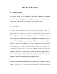
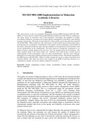
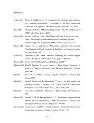
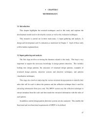
Chapter 3Figure 3.2: Detection and Locating LIPs in the study of Jiang et al. (2006). (Source:Y.-G. Jiang et al., 2006)Figure 3.2 illustrates keypoint detection and extraction stages as reported in the study ofY.-G. Jiang et al. (2006). Further visualisation of the above feature extraction stages canbe found in Figure 3.3.Figure 3.3: LIP distribution in a keyframe with different resolution in the study of Jianget al. (2006). (Source:Y.-G. Jiang et al., 2006)Figure 3.3 describes the distribution of LIPs with multi-resolution grid representation.The size of grids varies at different resolutions and thus the granularity of shapeinformation formed by LIP distribution changes according to the scale being considered.The first three colour moments of grids describe the shape-like information of LIPsacross resolutions. Each grid is physically viewed as a point characterized by momentsand weighted according to its levels of resolution. With this representation, basically akeyframe is treated as a bag of grid points. The similarity between keyframes is based66

Chapter 3upon the matching of grid points within and across resolutions depending on theirfeature distance and transmitted weights that can be evaluated with Earth Mover'sDistance (EMD). However, EMD is expensive and it has an exponential worst case withthe number of points (Y.-G. Jiang et al., 2006). Further, LIP generation inherits most ofthe computational costs with PCA-SIFT calculation.LIP-D (LIP Distribution) with 36 dimensional feature vector generates bag of gridpoints and utilises Support Vector Machine (SVM) classifier for visual classification.3.8. Video Visual Classifiers and ClassificationChapter 1 emphasises the importance of visual classifier in video visual contentdescription. There are different classifiers utilised by researchers in visual classificationbased on the type of visual feature. The advantages of reduction of feature space toclassification process are also discussed. A visual classifier performs mapping from avisual feature space to a discrete set of labels, that is mapping from low level syntacticvisual features to semantic visual concepts. Classifiers may either be fixed or learningclassifiers. Learning classifiers may in turn be divided into supervised and unsupervisedlearning classifiers. The accuracy and effectiveness of visual descriptiondepends on both selected visual feature and classification method. Selection of asuitable classification method for a certain visual syntactic feature can be done by usinga performance evaluation as discussed in our publication of this research (Ranathunga etal., 2009). That may be effective to a certain domain of visual concepts based on typevisuals, syntactic feature and classifier.Among video visual classifiers, Support Vector Machines (SVMs), Euclidean Distanceand k-NN based classification techniques are the most dominant (S. Gao et al., 2007;Hsu, Chang, & Lin, 2003; Lew et al., 2006; Lin et al., 2008; Lu, Zhao, & Zhang, 2008;Mittal, 2006; Smeulders & Kielmann, 2006; Snoek et al., 2005). There are some67

Chapter 3descriptors accompanied with its own classification method such as MPEG-7 DCD(Manjunath et al., 2001; Manjunath et al., 2002). Supervised classification task usuallyinvolves training and testing data which consist of some data instances. Each instance inthe training set contains one target value (class labels) and several attributes (features)(Hsu et al., 2003). The goal of a classifier is to produce a model that predicts targetvalue of data instances in the testing set based on the given attributes. Differentclassifiers use different properties and computational techniques in the classificationprocess. Efficiency and effectiveness of classification process depends on theclassification technique and the nature of low level syntactic features produced byfeature extractor.3.8.1. Euclidean Distance MeasureEuclidean distance is a popular and traditional similarity measure used for visualclassification (Datta et al., 2005; Lew et al., 2006; J. Liu et al., 2007; Lu et al., 2008;Mittal, 2006; Nguyen & Gillespie, 2003). It is used with a variety of low level visualfeatures such as histograms, Principal Components and Colour Moments. The basicrepresentation of this distance measure gives the variation between two feature vectors.Let X (X 1 , X 2 ,…X n ) and Y (Y 1 , Y 2 ,…Y n ) be the two feature vectors sharing same featurespace with n dimensions. Then the Euclidean Distance (d xy ) is defined as,dxy=n∑( ( X − Y ) 2 )(3.21)i=1iiThe classification is done by identifying the minimum distance with or without athreshold value. The major disadvantage of this similarity measure is that, thecomputational cost is high with the pair wise calculation in equation (3.21).68

Chapter 33.8.2. K-Nearest Neighbour Classificationk-Nearest Neighbour (k-NN) uses simple majority of target label categories with greatersimilarity in visual classification. The application of k-NN is always accompanied withsimilarity measure technique (Dementhon & Doermann, 2006; Lu et al., 2008). Theidentification of nearest neighbour algorithm involves the following steps:a. Determine parameter k, the number of nearest neighbours to be consideredb. Calculate the similarity between the feature vector of query-instance and all thelabelled feature vectors in training samplesc. Sort the similarity and determine nearest neighbours based on the k th closestsimilarityd. Gather the category labels of the k nearest neighbourse. Use simple majority of the label categories in the k nearest neighbours as thetarget label value of the query-instanceIn this method, a queried visual is assigned with the most common category among its knearest neighbours. The performance of the k-NN algorithm is influenced by three mainfactors which are the similarity metric used to locate the nearest neighbours, for anexample Euclidean distance; the decision rule used to derive a classification from the k-NN (threshold), and the number of neighbours used to classify the new sample.3.8.3. Support Vector Machine (SVM)Significant improvement of usage shows the dominancy of Support Vector Machine(SVM) based classification techniques in video content analysis (S. Gao et al., 2007;Hsu et al., 2003; Lew et al., 2006; Lin et al., 2008; Mittal, 2006; Smeulders &Kielmann, 2006; Snoek et al., 2005). The goal of SVM is to produce a model that69

Chapter 3predicts target value of data instances in the testing set by obtaining only featureattributes. SVMs are feed-forward networks that can be used for pattern classificationand nonlinear regression (Hsu et al., 2003). The main idea behind SVM is to construct ahyperplane that acts as a decision space in such a way that the margin of separationbetween positive and negative examples is maximized. This hyperplane is notconstructed in the input space, where the problem may not be linearly solvable, but inthe feature space where the problem is driven. This is generally referred to as theOptimal Hyperplane. Which is the property utilised by support vector machine inimplementation of the method of structural risk minimization (Hsu et al., 2003).Combination of SVMs for visual classification and 3D histograms for visual descriptionhave been used for the detection of semantic concepts (S. Gao et al., 2007). SVM doesnot incorporate domain-specific knowledge and it provides good generalizedperformance, which is a unique property among various different types of neuralnetworks.According to the description in (Hsu et al., 2003), the SVM classification is defined asfollows.Given a training set of instance-label pairs (x i , y i ), i = 1,….,l where x i є R n and y i є {1, -1} l , SVM requires the solution of the following optimization problem:minW , b,ξsubjected to1W2y ( Wξ ≥ 0.iiTW + C∑ξi,Ti=1φ(x ) + b)≥ 1−ξ ,ili(3.22)Training vectors x i are mapped into a higher dimensional space by the function φ. ThenSVM finds a linear separating hyperplane with the maximal margin in this higherdimensional space. W is weight vector and b are the constraints. C > 0 is the penaltyparameter of the error term. Slack variables of ξiare for handling non-separable data.70

Chapter 3Furthermore, K(x i , x j )≡φ(x i ) T φ(x j ) is called the kernel function. The linear kernel isdefined as K(x i , x j )≡x iTx j .3.9. SummaryThis chapter covers discussion on popular visual feature extraction and representationapproaches with reference to high dimensional visual feature approaches, 3D colourhistogram features, texture features, shape features, and local and key point features.Their strengths and weaknesses are also discussed. The dimensional reduction of visualfeature space is emphasised with several methods including MPEG-7 DCD, PCAmethods, and Colour Moments based methods. Finally, visual classification methodsand the relation between visual features and classifiers are described with relevantclassification methods.71