Control of a Bicycle Using Virtual Holonomic Constraints

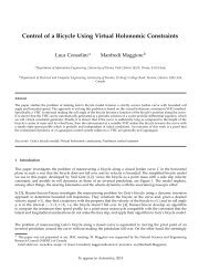
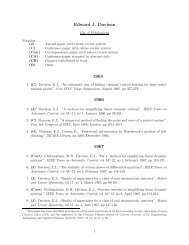
Control of a Bicycle Using Virtual Holonomic ConstraintsLuca Consolini, Manfredi MaggioreAbstract— The problem of making a bicycle trace a strictlyconvex Jordan curve with bounded roll angle and boundedspeed is investigated. The problem is solved by enforcing avirtual holonomic constraint which specifies the roll angle of thebicycle as a function of its position along the curve. It is shownthat virtual holonomic constraints can be generated as periodicsolutions of a scalar periodic differential equation. Finally, itis shown that if the mean curvature of the path is sufficientlysmall the virtual holonomic constraint can be asymptoticallystabilised and the speed of the bicycle is asymptotically periodic.I. INTRODUCTIONThis paper investigates the problem of maneuvering abicycle along a closed Jordan curve C in the horizontal planein such a way that the bicycle does not fall over and itsvelocity is bounded. The simplified bicycle model we use inthis paper, developed by Neil Getz [1], [2], views the bicycleas a point mass with a side slip velocity constraint, andmodels its roll dynamics as those of an inverted pendulum,see Figure 1. The model neglects, among other things, thewheels dynamics and the associated gyroscopic effect. Thedynamics of Getz’s bicycle when the contact point of the rearwheel is made to follow the curve C are Euler-Lagrange.In [3], Hauser-Saccon-Frezza investigate the maneuveringproblem for Getz’s bicycle using a dynamic inversion approachto determine bounded roll trajectories. They constrainthe bicycle on the curve and, given a desired velocity signalv(t), they find a trajectory with the property that the velocityof the bicycle is v(t) and its roll angle ϕ is in the interval(−π/2, π/2), i.e, the bicycle doesn’t fall over. In [4], Hauser-Saccon develop an algorithm to compute the minimum-timespeed profile for a point-mass motorcycle compatible withthe constraint that the lateral and longitudinal accelerationsdo not make the tires slip, and apply their algorithm to Getz’sbicycle model.The problem of maneuvering Getz’s bicycle along a closedcurve is equivalent to moving the pivot point of an invertedpendulum around the curve without making the pendulumfall over. On the other hand, the seemingly different problemof maneuvering Hauser’s PVTOL aircraft [5] along a closedcurve in the vertical plane can be viewed as the problem ofmoving the pivot of an inverted pendulum around the curvewithout making the pendulum fall over. The two problemsL. Consolini is with the Department of Information Engineering,University of Parma, Viale Usberti 181/A, Parma, 43124 Italy,E-mail: lucac@ce.unipr.itM. Maggiore is with the Department of Electrical and Computer Engineering,University of Toronto, 10 King’s College Road, Toronto, Ontario,M5S 3G4, Canada. E-mail: maggiore@control.utoronto.ca.M. Maggiore was supported by the Natural Sciences and EngineeringResearch Council (NSERC) of Canada.are, therefore, closely related, the main difference being thefact that in the former case the pendulum lies on a planewhich is orthogonal to the plane of the curve, while inthe latter case it lies on the same plane. In [6], the pathfollowing problem for the PVTOL was solved by enforcinga virtual holonomic constraint which specifies the roll angleof the PVTOL as a function of its position on the curve.In this paper we follow a similar approach for the bicyclemodel and impose a virtual holonomic constraint relating thebicycle’s roll angle to its position along the curve, but ratherthan finding one feasible virtual constraint, we show howto generate a class of feasible virtual constraints as periodicsolutions of a scalar periodic differential equation which wecall the virtual constraint generator. We show that if thecurvature of the path is sufficiently small compared to theheight of the bicycle’s centre of mass, then on the constraintmanifold the velocity of the bicycle converges exponentiallyto a periodic profile. In other words, the bicycle traversesthe entire curve with bounded speed and its speed profileis asymptotically periodic. Finally, we design a controllerwhich exponentially stabilises the virtual constraint manifoldand recovers the asymptotic properties of the bicycle on theconstraint manifold just described.The idea of virtual holonomic constraint is a usefulparadigm for the control of oscillations and goes well beyondthe example investigated in this paper. To the best of ourknowledge, this notion originated with the work of Grizzleand collaborators on biped locomotion (e.g., [7] and [8]). Therecent work in [9], [10], [11] investigated virtual holonomicconstraints for Euler-Lagrange systems. There, an integralof motion for the dynamics on the virtual constraint wasgiven explicitly, and a methodology to stabilise desired limitcycles on the virtual constraint manifold was given basedon a time-varying linearization of the system on the limitcycle. In [12], this ideas were applied to the stabilisationof oscillations in the Furuta pendulum. In [13], we gaveconditions for a virtual holonomic constraint to be feasible,and we exposed the role of the virtual constraint generatorin producing feasible virtual constraints that can always belocally exponentially stabilised. We also presented sufficientconditions in order that the reduced system describing themotion on the virtual constraint manifold be Euler-Lagrange.The bicycle model in this paper does not meet the sufficientconditions of [13]; in fact, we will show that the reduced systemis not Euler-Lagrange. Getz’s bicycle model is thereforean example showing that the reduced motion of an Euler-Lagrange system subjected to a virtual holonomic constraintmay not be Euler-Lagrange. See Remark 3.4 for more details.

ϕmδIn order to derive the constrained dynamics, suppose that(x(0), y(0)) ∈ C, i.e., (x(0), y(0)) = σ(s 0 ), for some s 0 ∈R modT. A point σ(s(t)) moving on C has linear velocityv(t) = ‖σ ′ (s(t))‖ṡ(t) (2)and accelerationψ(x, y)bhp˙v(t) = ‖σ ′ (s(t))‖¨s(t) +ṡ 2 (t)‖σ ′ (s(t))‖ σ′ (s(t)) ⊤ σ ′′ (s(t)). (3)Therefore, for an arbitrary velocity signal v(t), (x(t), y(t))traverses C with velocity v(t) if and only if (x(0), y(0)) ∈ C,(ẋ(0), ẏ(0)) is tangent to C, and the steering angle δ(t)( is chosen to be δ(t) = arctan[p κ(s(t))], where s(t) =∫ t(s(τ))‖]dτ)0 [v(τ)/‖σ′ modT, so thatFig. 1.Getz’s bicycle model.We adopt the notational conventions in [3] to describe thesimplified bicycle model depicted in Figure 1:• (x, y) - coordinates of the point of contact of the rearwheel• ϕ - roll angle• ψ - yaw angle• δ - projected steering angle on the (x, y) plane• b - distance between the projection of the centre of massand the point of contact of the rear wheel• p - wheel base• h - pendulum length• v - forward linear velocity of the bicycle• f - reaction force of the ground on the rear wheel.We will denote ¯κ = tanδ/p = ˙ψ/v. For a given velocitysignal v(t) and steering angle signal δ(t), ¯κ(t) representsthe curvature of the path (x(t), y(t)) traced by the pointof contact of the rear wheel. The model of the bicycle inFigure 1 was presented in [2] and is given by[¨ϕ˙v]M = F + B[˙¯κf], (1)where, letting s ϕ = sin ϕ and c ϕ = cosϕ,[ ]h2bhcM =ϕ¯κbhc ϕ¯κ 1 + (b 2 + h 2 s 2 ϕ)¯κ 2 ,− 2h¯κs ϕ[]ghsF = ϕ − (1 − h¯κs ϕ )hc ϕ¯κv 2(1 − h¯κs ϕ )2hc ϕ¯κv ˙ϕ + bh¯κs ϕ ˙ϕ 2 ,[]− bhcB =ϕ v 0− (b 2¯κ .− hs ϕ (1 − h¯κs ϕ ))v 1/mConsider a C 3 closed Jordan curve C in the (x, y) planewith regular parametrization σ(s) : R modT → R 2 (T is theperiod of the function σ), not necessarily unit speed. Let κ(s)denote the signed curvature of C. Throughout this paper, weassume the following.Assumption 1: The curve C is strictly convex, i.e., κ(s) >0 for all s ∈ R modT.In this paper we investigate the dynamics of the bicycle whenthe point (x, y) is constrained to move along the curve C.¯κ(t) = κ(s(t)). (4)The motion of the bicycle on the curve C is thus found bysubstituting (2), (3), (4) in (1):[] [ ]¨ϕ˜M‖σ ′ ‖¨s + (σ′ ) ⊤ σ ′′ = ˜F 0+ f , (5)‖σ ′ ‖ ṡ2 1/mwhere ˜M = M|¯k=k(s) and( [ ) ∣1 ˜F = F + B k0]′ (s)ṡ.∣∣∣¯k=k(s),v=‖σ ′ (s)‖ṡThe motion of the bicycle on C in (5) is an Euler-Lagrangesystem with configuration variables (ϕ, s) and LagrangianL = T − V , withT = 1 [2 [ ˙ϕ ‖σ′ (s)‖ṡ] ˜M˙ϕ‖σ ′ (s)‖ṡ], V = gh cosϕ.Since the control force f enters nonsingularly in the ¨sequation, we can define a feedback transformation for fin (5) such that ¨s = u, where u is the new control input.With this transformation, the motion of the bicycle on Creads as[h¨ϕ = gs ϕ − (1 − hκ(s)s ϕ )κ(s)‖σ ′ (s)‖ + bκ ′ (s)+ bκ(s) ]‖σ ′ (s)‖ 2 σ′ (s) ⊤ σ ′′ (s) c ϕ ‖σ ′ (s)‖ṡ 2 − bκ(s)c ϕ ‖σ ′ (s)‖u¨s = u.(6)Letting q = (ϕ, s), the state space is X = {(q, ˙q) ∈ S 1 ×(R modT) × R 2 }. In our simulations we will use h = 1 mand b = 1.5 m.Remark 1.1: If σ(s) is a unit speed parametrization of C,then the first differential equation in (6) reduces to[]h¨ϕ = gs ϕ − (1 −hκ(s)s ϕ )κ(s)+bκ ′ (s) c ϕ ṡ 2 −bκ(s)c ϕ u.The objective of this paper is to solve the followingManeuvering Problem. Find a feedback u(q, ˙q) forsystem (6) such that there exists a set of initial conditions Ωwith the property that, for all (q(0), ˙q(0)) ∈ Ω, the bicycledoes not overturn, i.e., |ϕ(t)| < π/2 for all t ≥ 0, andtraverses the entire curve C in one direction, i.e., there exists2

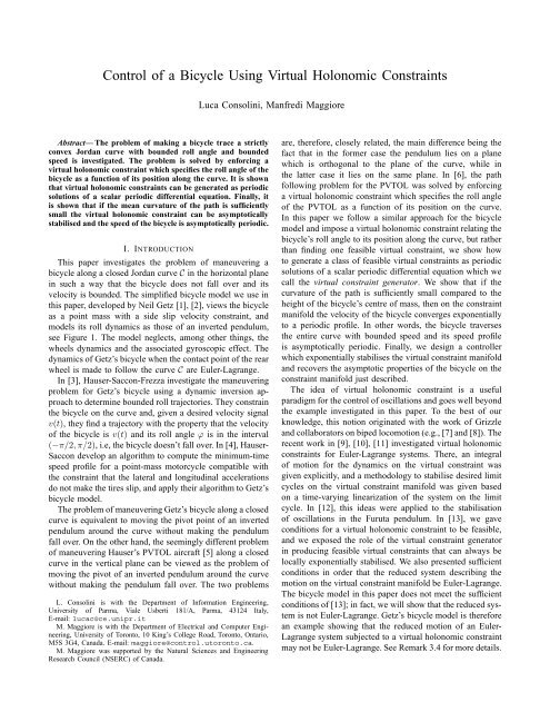
¯t > 0 such that |ṡ(t)| > 0 for all t ≥ ¯t. Moreover, the speedṡ(t) of the bicycle on C should remain bounded.Our solution of this problem relies on the notion of virtualholonomic constraint.Definition 1.2: A function ϕ = Φ(s), Φ : R modT →S 1 is a virtual holonomic constraint for system (6) if theconstraint manifoldΓ = {(q, ˙q) ∈ X : ϕ = Φ(s), ˙ϕ = Φ ′ (s)ṡ}is controlled invariant, i.e., there exits a smooth feedbacku(q, ˙q) rendering it invariant.The constraint manifold Γ is the collection of all thosephase curves of (6) such that ϕ(t) = Φ(s(t)) for all tfor which the solution is defined. It is a two-dimensionalsubmanifold of X parametrized by (s, ṡ), and thereforediffeomorphic to the cylinder (R modT) × R. Our approachto solving the maneuvering problem is to look for virtualholonomic constraints ϕ = Φ(s) such that |Φ(s)| < π/2for all s ∈ R modT. The advantage of this approach, asopposed to searching for individual bounded roll trajectories,is that each virtual constraint Φ provides a family ofbounded roll trajectories corresponding to arbitrary choicesof (s(0), ṡ(0)) ∈ (R modT) × R.II. THE VIRTUAL CONSTRAINT GENERATORIn this section we show that virtual holonomic constraintsfor (6) can be generated as solutions of a first-order differentialequation, which we call the virtual constraint generator.This idea was first presented in our previous work [13]. Webegin with a sufficient condition for a function Φ to be afeasible virtual holonomic constraint for (6).Lemma 2.1: A C 1 function ϕ = Φ(s), R modT → S 1 isa virtual holonomic constraint for system (6) ifΦ ′ (s) + h −1 bκ(s)‖σ ′ (s)‖ cosΦ(s) ≠ 0 (7)for all s ∈ R modT.Proof: Viewing the function ϕ − Φ(s) as an outputof system (6), condition (7) is simply the requirement thatsaid output has a well-defined uniform relative degree 2 on{ϕ − Φ(s) = 0}. The associated zero dynamics manifold isprecisely Γ, and it is controlled invariant.The foregoing lemma inspires the following observation.Instead of guessing a virtual constraint and checking whetherit is feasible, as in the lemma, one could use (7) to generatefeasible virtual holonomic constraints. More precisely, letr = h −1 b and consider the scalar differential equationdΦds = −rκ(s)‖σ′ (s)‖ cosΦ + δ(s). (8)Since s is a cyclic variable in R modT, the above is a T -periodic differential equation. If, for some δ(s) ≠ 0, (8)has a T -periodic solution Φ(s), then in light of Lemma 2.1,ϕ = Φ(s) is a virtual holonomic constraint. Therefore, onecan think of differential equation (8) as a virtual holonomicconstraint generator, for which one is to pick δ(s) suchthat a periodic solution exists. Such problem of existenceof periodic solutions is addressed in the next proposition,whose proof is omitted due to space limitations.Proposition 2.2: Set δ(s) = ǫµ(s), where µ : R modT →R is a T -periodic and locally Lipschitz function such thatµ(s) > 0 for all s ∈ R modT, and let( )K + =K − =maxs∈R mod Tmins∈R mod Tµ(s)κ(s)‖σ ′ (s)‖(µ(s)κ(s)‖σ ′ (s)‖,).Then, for any Φ 0 ∈ (0, π/2) mod2π and s 0 ∈ R modT,(i) there exists a uniqueǫ ∈ [ǫ − , ǫ + ] = [(r cosΦ 0 )/K + , (r cosΦ 0 )/K − ],such that the solution of (8) with δ(s) = ǫµ(s) andinitial condition Φ(s 0 ) = Φ 0 is T -periodic.(ii) If µ(s) is chosen so that K + /K − < (cosΦ 0 ) −1 , thenthe image of the T -periodic solution Φ(s) in part (i) iscontained in the interval(Φ − , Φ + ) =(cos −1( K +K − cosΦ 0), cos −1( K − ) )K + cosΦ 0 ,which is a subset of (0, π/2).Remark 2.3: By choosing µ(s) = κ(s)‖σ ′ (s)‖, we haveK + = K − = 1, ǫ + = ǫ − = r cosΦ 0 . In this case, theproposition above implies that, for all Φ 0 ∈ (0, π/2), settingδ(s) = rκ(s)‖σ ′ (s)‖ cosΦ 0 , the virtual constraint generatorhas a T -periodic solution Φ(s) whose image is in the interval(0, π/2) mod2π. As a matter of fact, one can readily verifythat the solution in question is constant, Φ(s) = Φ 0 , whichcorresponds to the situation when the bicycle has a constantroll angle as it travels around C. The proposition providesgreat flexibility in finding virtual holonomic constraints withthe property that the roll angle is confined within the interval(0, π/2) mod2π. All such constraints are compatible with themaneuvering problem.Example 2.4: Suppose C is an ellipse with major semiaxisA, minor semiaxis B, and 2π-periodic parametrizationσ(s) = (Acos s, B sin s), with A = 15, B = 5. Thecurvature is κ(s) = AB/(A 2 sin 2 s + B 2 cos 2 s) 3/2 . For theinitial condition of the virtual constraint generator, we pickΦ(0) = π/3. Following Proposition 2.2, we need to choosea 2π-periodic function µ(s) > 0, set δ(s) = ǫµ(s), and findthe unique value of ǫ > 0 guaranteeing that the solutionwith initial condition Φ(0) = π/3 is 2π-periodic. There ismuch freedom in the choice of µ(s). For instance, pickingµ(s) = 1, we numerically find ǫ ≈ 0.927. The correspondingvirtual holonomic constraint is depicted in Figure 2. Thecondition, in Proposition 2.2(ii), that K + /K − < (cosφ 0 ) −1is very conservative. Indeed, with our choice of µ we haveK + = 3, K − = 1/3 and thus the condition is violated. Yet,the image of the virtual constraint is contained in the interval(0, π/2).III. MOTION ON THE CONSTRAINT MANIFOLDHaving chosen δ(s) as in Proposition 2.2(ii) and an associatedvirtual holonomic constraint ϕ = Φ(s) satisfying (8),3

pi/2pi/4Φ(s)00 pi/2 pi 3pi/2 2piFig. 2. Virtual holonomic constraint for the ellipse in Example 2.4.the next step is to analyse the dynamics on the constraintmanifold Γ = {(q, ˙q) ∈ X : ϕ = Φ(s), ˙ϕ = Φ ′ (s)ṡ}. Theseare the zero dynamics of (6) with output function ϕ − Φ(s).The feedback making Γ invariant is found by imposing thatddt [Φ′ (s)ṡ] ∣ Γ= ¨ϕ ∣ Γ. Expanding both sides of the equationabove, using identity (8), and the fact that δ(s) ≠ 0, weobtain the feedback making Γ invariant[− ṡ2Φ ′′ + 1 δ h ((1 − hκ sin Φ)κ‖σ′ ‖ + bκ ′]+ bκσ ′ ⊤ σ ′′ /‖σ ′ ‖ 2 )‖σ ′ ‖ cosΦ .u = h−1 g sinΦδSubstituting this feedback in the s dynamics we get thedynamics on Γ,where¨s = Ψ 1 (s) + Ψ 2 (s)ṡ 2 , (9)Ψ 1 (s) = h−1 g sin Φ(s)δ(s)Ψ 2 (s) = − 1 [Φ ′′ (s) + 1 δ(s) h ((1 − hκ(s)sin Φ(s))κ(s)‖σ′ (s)‖]+ bκ ′ (s) + bκ(s)σ ′ (s) ⊤ σ ′′ (s)/‖σ ′ (s)‖ 2 )cosΦ(s)‖σ ′ (s)‖ .(10)System (9) describes the motion on Γ in the followingsense. If the bicycle is initialized on the curve C, withinitial roll angle ϕ(0) = Φ(s 0 ) for some s 0 ∈ R modT,and with initial angular velocity ˙ϕ(0) = Φ ′ (s 0 )ṡ 0 for someṡ 0 ∈ R, then the bicycle remains on C, its roll angle satisfiesϕ(t) = Φ(s(t)) for all t ≥ 0, and the position s and velocityṡ of the bicycle on C evolve according to (9). In order forthe virtual holonomic constraint to be compatible with themaneuvering problem, we need to verify whether or not thebicycle traverses the entire curve C with bounded speed, i.e.,that there exist ¯t > 0, ǫ > 0 such that ṡ(t) > ǫ > 0 for allt ≥ ¯t, and limsup t→∞ ṡ(t) < ∞. The next result exploresgeneral properties of systems of the form (9).Proposition 3.1: Consider a differential equation of theform (9), where Ψ 1 and Ψ 2 are T -periodic and locallyLipschitz∫functions such that Ψ 1 (s) > 0 for all s andT0 Ψ 2(s)ds < 0. Then, there exists a real-valued T -periodicfunction ν(s), with ν(s) > 0, such that the set R = {(s, ṡ) :ṡ = ν(s)} is exponentially stable for (9), with domainof attraction containing the set D = {(s, ṡ) : ṡ ≥ 0}.sMoreover, for all initial conditions in {(s, ṡ) : ṡ ≥ 0}, thefunction t ↦→ ν(s(t)) is periodic and so ṡ(t) is asymptoticallyperiodic.Remark 3.2: It can be shown that the domain of attractionof the set R in the foregoing proposition is {(s, ṡ) : ṡ >−ν(s)}.Proof: The set {(s, ṡ) : ṡ ≥ 0} is positively invariantfor (9) because ¨s|ṡ=0 = Ψ 1 (s) > 0 by assumption. Since theinequality is strict, we have ṡ(t) > 0 for all t > 0. In the restof the proof we will restrict initial conditions on D. Lettingz = ṡ 2 , we have ż = 2ṡ(Ψ 1 (s) + Ψ 2 (s)z). Since ṡ > 0 forall t > 0, we can use s as a time variable:dzds = 2Ψ 1(s) + 2Ψ 2 (s)z. (11)The above is a scalar linear T -periodic system. As before,if z(s 0 ) ≥ 0, then z(s) > 0 for all s > s 0 . Letting φ(s) =exp(2 ∫ s0 Ψ 2(τ)dτ), the solution of the linear system withinitial condition z(s 0 ) isz(s) = φ(s − s 0 )z(s 0 ) + 2∫ ss 0φ(s)φ −1 (τ)Ψ 1 (τ)dτ.System (11) has a T -periodic solution if and only if thereexists z 0 such that z 0 = z(s 0 ) = z(s 0 + T), i.e, z 0 =φ(T)z 0 +2 ∫ s 0+Ts 0φ(s 0 +T)φ −1 (τ)Ψ 1 (τ)dτ. Using the factthat φ(s + u) = φ(s)φ(u), the condition becomes∫ Tz 0 = φ(T)z 0 + 2 φ(T)φ −1 (τ)Ψ 1 (τ)dτ. (12)0By assumption, 0 < φ(T) < 1, so the equation abovehas a unique solution z 0 > 0 and (11) has a unique T -periodic solution ¯z(s) > 0. Letting ˜z(k) = z(s 0 + kT) − z 0and using identity (12), we have ˜z(k + 1) = φ(T)˜z(k).Since φ(T) < 1, the origin of this discrete-time systemis globally exponentially stable, proving that the T -periodicsolution ¯z(s) is globally exponentially stable for (11). Letν(s) = √¯z(s) and return to system (9). For all initialconditions (s(0), ṡ(0)) ∈ D, we have ṡ(t) > 0 for all t > 0,and ṡ(t) = √ z(s(t)), where z(s) is the solution of (11)with initial condition z(s(0)) = ṡ(0) 2 . Since ¯z(s) is globallyexponentially stable for (11), R is exponentially stable for (9)with domain of attraction containing D.It remains to be shown that t ↦→ ν(s(t)) is periodic.Consider the scalar differential equation ṡ = √¯z(s), whosevector field is T -periodic. Denote by ̺(t, s 0 ) its solutionwith initial condition s(0) = s 0 at time t. For all s 0 ,̺(t, s 0 + T) = ̺(t, s 0 ) + T . Indeed, ̺(0, s 0 ) + T = s 0 + Tandddt [̺(t, s 0) + T] = √¯z(̺(t, s 0 )) = √¯z(̺(t, s 0 ) + T).Next, since ṡ = √¯z(s) > 0, there exist unique times ¯t > 0and t 0 such that ̺(¯t, 0) = T and ̺(t 0 , 0) = s 0 , and̺(t + ¯t, s 0 ) = ̺(t + ¯t + t 0 , 0) = ̺(t + t 0 , T)= ̺(t + t 0 , 0) + T = ̺(t, s 0 ) + T.4

It then follows that for all t and s 0 , d̺(t + ¯t, s 0 )/dt =d̺(t, s 0 )/dt or, what is the same, for any s 0 , t ↦→ ν(s(t)) isperiodic.We now show that if the curvature of C satisfies an integralbound, the bicycle satisfies the hypotheses of Proposition 3.1,and so the motion on the constraint manifold satisfies therequirements of the maneuvering problem.Proposition 3.3: If the curvature of C satisfies the inequality∫1 Tκ(s)ds 0, such that the closedorbit of (9) R = {(s, ṡ) : ṡ = ν(s)} is exponentiallystable, and D = {(s, ṡ) : ṡ ≥ 0} lies in its domain ofattraction. Moreover, for all initial conditions in D, ṡ(t) isasymptotically periodic.Remark 3.4: The existence of the isolated closed orbit Rof (9) which is exponentially stable implies that the reducedmotion on the constraint manifold Γ is not Euler-Lagrange.Getz’s bicycle is therefore an example of an Euler-Lagrangesystem for which there is a virtual holonomic constraint suchthat the reduced motion is not Euler-Lagrange.Proof: By Proposition 2.2(i), the virtual constraintsatisfies Φ(s) ∈ (0, π/2), and so sin Φ(s) > 0. Sinceδ(s) > 0 it follows that Ψ 1 (s) > 0. Using equality (8),we haveΦ ′′ = δ ′ − rκ ′ ‖σ ′ ‖ cosΦ − (rκ‖σ ′ ‖) 2 sinΦcosΦ+ rκ‖σ ′ ‖δ sin Φ − rκσ ′ ⊤ σ ′′ /‖σ ′ ‖.Substituting in the expression for Ψ 2 in (10) we getΨ 2 = − δ′δ − κ‖σ′ ‖[bδ sin Φ − ‖σ ′ ‖ cosΦδh·(κ sin Φ b2 + h 2 ) ]− 1h≤ − δ′δ + κ‖σ′ ‖ 2cosΦ(κ sinΦ b2 + h 2 )− 1 .δhhSince ∫ T0 δ′ (s)/δ(s) = lnδ(T) − lnδ(0) = 0, using thebounds in Proposition 2.2(ii), we have∫ T ∫ Tκ‖σ ′ ‖ 2Ψ 2 (s)ds ≤ cosΦ(κ sinΦ b2 + h 2 )− 1 ds00 δhh( κ‖σ ′ ‖ 2 ) ∫ T≤ max cosΦ(κ(s) − b2 + h 2 )− 1 dss δh0 h( κ‖σ ′ ‖ 2 ) (b≤ max cosΦ − 2 + h 2 ∫ )Tκ(s)ds − T < 0.s δhhRemark 3.5: If the parametrization σ(s) of C has unitspeed (i.e., ‖σ ′ (s)‖ = 1), then T is the length of C, andthe integral (1/T) ∫ Tκ(s)ds is equal to (turning number of0C)×2π/T . The turning number is the number of revolutions0ṡ6420−2−4R−60 1 2 3 4 5 6Fig. 3. Phase portrait of the dynamics on Γ and set R for the ellipse inExample 2.4. The shaded region is the domain of attraction of R.that the tangent vector to C makes as a point is moved oncearound C. For a Jordan curve, the turning number is ± 1.Example 3.6: We return to ellipse of Example 2.4 and thevirtual constraint displayed in Figure 2. For this example,(1/2π) ∫ 2πκ(s)ds ≈ 0.142, and h/(b 2 + h 2 ) = 0.308 and0thus∫(13) is satisfied. Indeed, one can numerically check thatT0 Ψ 2(s)ds ≈ −27.5 < 0, and Proposition 3.1 applies. Thephase portrait of the dynamics on the constraint manifoldis displayed in Figure 3. The figure illustrates the set R,corresponding to the steady-state velocity profile of thebicycle on Γ. The domain of attraction of R, shaded in thefigure, is the set {(s, ṡ) : ṡ > −ν(s)}, as pointed out inRemark 3.2.Example 3.7: Suppose C is a circle of radius R. The curvatureis constant, κ = 1/R. For any Φ 0 ∈ (0, π/2), pickingδ = (r/R)cos Φ 0 , as in Remark 2.3, we obtain the constantvirtual constraint Φ(s) = Φ 0 . Equation (11) becomesdz/ds = (gR)/(hr)tan Φ 0 − 1/(hr)(1 − (h/R)sinΦ 0 )z.The above is a linear time-invariant system with constantinput which is stable if R > h sin Φ 0 . The periodic solution¯z(s) in this case is simply the equilibrium of the systemabove, ¯z = gR 2 tan Φ 0 /(R −h sinΦ 0 ), and thus the asymptoticvelocity of the bicycle on Γ is constant, and reads asν = R √ g tanΦ 0 /(R − h sin Φ 0 ). It can be verified that νis an increasing function of Φ 0 . The conclusion is that thebicycle can go around the circle with any constant roll anglein the interval (0, π/2). The larger is the roll angle Φ 0 , thehigher is the asymptotic speed of the bicycle.IV. SOLUTION OF THE MANEUVERING PROBLEMTheorem 4.1: Suppose that the mean curvature of C satisfiesinequality (13). If Φ(s) is a virtual holonomic constraintsatisfying (7) and such that Φ(s) ∈ (0, π/2) for all s ∈R modT, then the feedbacku = 1∆(q)s( 1(h gs ϕ − Φ ′′ + 1 h)+ bκσ′⊤ σ ′′‖σ ′ ‖ 2 )c ϕ ‖σ ′ ‖((1 − hκs ϕ )κ‖σ ′ ‖ + bκ ′)ṡ 2 + K 1 e + K 2 ė ,(14)where ∆(q) = Φ ′ (s) + h −1 bκ(s)c ϕ ‖σ ′ (s)‖, e = ϕ − Φ(s),ė = ˙ϕ −Φ ′ (s)ṡ, and K 1 , K 2 are positive design parameters,5

solves the maneuvering problem and has the followingproperties:(i) The constraint manifold Γ is invariant and locally exponentiallystable for the closed-loop system (6), (14).(ii) There exists a C 1 and T -periodic function ν(s) :R modT → R, with ν(s) > 0 such that the setR = {(q, ˙q) ∈ Γ : ṡ = ν(s)} is asymptotically stablefor the closed-loop system and its domain of attractionis a neighbourhood of the set {(q, ˙q) ∈ Γ : ṡ > 0}.(iii) For initial conditions in the domain of attraction of R,the bicycle traverses the entire curve C and its speed isasymptotically periodic.Proof: By construction, Φ(s) satisfies (7) and, as arguedin the proof of Lemma 2.1, system (6) with output e hasuniform relative degree 2 on Γ. The feedback (14) is afeedback linearizing controller making the origin of the (e, ė)subsystem, and hence Γ, exponentially stable, proving part(i).As for part (ii), we know from Proposition 3.3 that thereexists a T -periodic function ν(s) such that the set R isexponentially stable for the restriction of the dynamics on Γ.In order to prove that R is asymptotically stable for initialconditions outside of Γ, note that R is a one-dimensionalsubmanifold of Γ diffeomorphic to S 1 , and hence compact.Owing to the reduction principle for asymptotic stabilityof compact sets (see [14], [15]), the asymptotic stabilityof R relative to Γ together with the asymptotic stabilityof Γ implies that R is asymptotically stable for (6). ByProposition 3.3, its domain of attraction contains the set{(q, ˙q) ∈ Γ : ṡ > 0}.Finally, concerning part (iii), since on R we have ṡ =ν(s) > 0, for all initial conditions in the domain of attractionof R there exists a time ¯t > 0 such that ṡ(t) > 0 for all t ≥ ¯t,and hence the bicycle traverses the entire curve C. Since Ris diffeomorphic to S 1 , since it is asymptotically stable, andon it solutions are periodic, R is a stable limit cycle of theclosed-loop system. Therefore, solutions in the domain ofattraction of R are asymptotically periodic.Example 4.2: We return to example of the ellipse, withthe virtual constraint depicted in Figure 2. The simulationresults for the closed-loop system with controller (14) andK 1 = 100, K 2 = 10 are shown in Figures 4, 5 forthe initial condition (ϕ(0), ˙ϕ(0), s(0), ṡ(0)) = (0, 0, 0, 1).Figure 4 illustrates the exponential convergence of ϕ(t) tothe constraint Φ(s(t)). Figure 5 displays the projection ofthe phase curve on the (s, ṡ) plane and its convergence tothe submanifold R.REFERENCES[1] N. Getz, “Control of balance for a nonlinear nonholonomic nonminimumphase model of a bicycle,” in American Control Conference,1994, pp. 148–151.[2] N. Getz and J. Marsden, “Control for an autonomous bicycle,” inIEEE International Conference on Robotics and Automation, vol. 2,May 1995, pp. 1397–1402 vol.2.[3] J. Hauser, A. Saccon, and R. Frezza, “Achievable motorcycle trajectories,”in IEEE Conference on Decision and Control, December 2004.[4] J. Hauser and A. Saccon, “Motorcycle modeling for high-performancemaneuvering,” IEEE Control Systems Magazine, pp. 89–105, October2006.pi/23pi/8pi/4pi/8Φ(s(t))ϕ(t)00 1 2 3 4 5 6Fig. 4. Simulation of the closed-loop system for the ellipse example. Thesolution converges to the constraint manifold Γ.ṡ6420−2−4−60 1 2 3 4 5 6tRFig. 5. Simulation of the closed-loop system for the ellipse example. Thesolution converges to the submanifold R ⊂ Γ.[5] J. Hauser, S. Sastry, and G. Meyer, “Nonlinear control design forslightly non-minimum phase systems: Applications to V/STOL aircraft,”Automatica, vol. 28, no. 4, pp. 665–679, 1992.[6] C. Nielsen, L. Consolini, M. Maggiore, and M. Tosques, “Path followingfor the pvtol: A set stabilization approach,” in IEEE Conferenceon Decision and Control, Cancun, Mexico, December 2008.[7] F. Plestan, J. Grizzle, E. Westervelt, and G. Abba, “Stable walking of a7-DOF biped robot,” IEEE Transactions on Robotics and Automation,vol. 19, no. 4, pp. 653–668, 2003.[8] E. Westervelt, J. Grizzle, and D. Koditschek, “Hybrid zero dynamics ofplanar biped robots,” IEEE Transactions on Automatic Control, vol. 48,no. 1, pp. 42–56, 2003.[9] C. Canudas-de-Wit, “On the concept of virtual constraints as a toolfor walking robot control and balancing,” Annual Reviews in Control,vol. 28, pp. 157–166, 2004.[10] A. Shiriaev, J. Perram, and C. Canudas-de-Wit, “Constructive toolfor orbital stabilization of underactuated nonlinear systems: Virtualconstraints approach,” IEEE Transactions on Automatic Control.,vol. 50, no. 8, pp. 1164–1176, August 2005.[11] L. Freidovich, A. Robertsson, A. Shiriaev, and R. Johansson, “Periodicmotions of the Pendubot via virtual holonomic constraints: Theory andexperiments,” Automatica, vol. 44, pp. 785–791, 2008.[12] A. Shiriaev, L. Freidovich, A. Robertsson, R. Johansson, and A. Sandberg,“Virtual-holonomic-constraints-based design of stable oscillationsof Furuta pendulum: Theory and experiments,” IEEE Transactionson Robotics, vol. 23, no. 4, pp. 827–832, 2007.[13] L. Consolini and M. Maggiore, “Virtual holonomic constraints forEuler-Lagrange systems,” in Proceedings of the 8th IFAC Symposiumon Nonlinear Control Systems (NOLCOS), Bologna, Italy, 2010.[14] M. El-Hawwary and M. Maggiore, “Reduction principles for stabilityof closed sets,” 2009, submitted to Systems and Control Letters.[15] ——, “Reduction principles and the stabilization of closed sets forpassive systems,” 2009, http://arxiv.org/abs/0907.0686v1.s6