download - Professor Carol Alexander

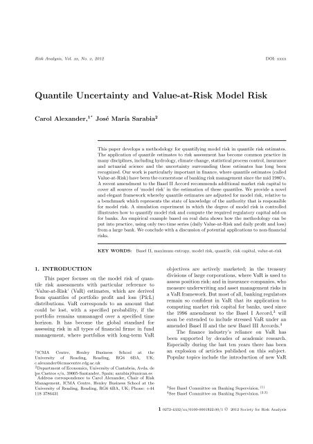
Risk Analysis, Vol. xx, No. x, 2012DOI: xxxxQuantile Uncertainty and Value-at-Risk Model RiskCarol Alexander, 1⋆ José María Sarabia 2This paper develops a methodology for quantifying model risk in quantile risk estimates.The application of quantile estimates to risk assessment has become common practice inmany disciplines, including hydrology, climate change, statistical process control, insuranceand actuarial science and the uncertainty surrounding these estimates has long beenrecognized. Our work is particularly important in finance, where quantile estimates (calledValue-at-Risk) have been the cornerstone of banking risk management since the mid 1980’s.A recent amendment to the Basel II Accord recommends additional market risk capital tocover all sources of ‘model risk’ in the estimation of these quantiles. We provide a noveland elegant framework whereby quantile estimates are adjusted for model risk, relative toa benchmark which represents the state of knowledge of the authority that is responsiblefor model risk. A simulation experiment in which the degree of model risk is controlledillustrates how to quantify model risk and compute the required regulatory capital add-onfor banks. An empirical example based on real data shows how the methodology can beput into practice, using only two time series (daily Value-at-Risk and daily profit and loss)from a large bank. We conclude with a discussion of potential applications to non-financialrisks.KEY WORDS:Basel II, maximum entropy, model risk, quantile, risk capital, value-at-risk1. INTRODUCTIONThis paper focuses on the model risk of quantilerisk assessments with particular reference to‘Value-at-Risk’ (VaR) estimates, which are derivedfrom quantiles of portfolio profit and loss (P&L)distributions. VaR corresponds to an amount thatcould be lost, with a specified probability, if theportfolio remains unmanaged over a specified timehorizon. It has become the global standard forassessing risk in all types of financial firms: in fundmanagement, where portfolios with long-term VaR1 ICMA Centre, Henley Business School at theUniversity of Reading, Reading, RG6 6BA, UK;c.alexander@icmacentre.rdg.ac.uk2 Department of Economics, University of Cantabria, Avda. delos Castros s/n, 39005-Santander, Spain; sarabiaj@unican.es⋆ Address correspondence to Carol Alexander, Chair of RiskManagement, ICMA Centre, Henley Business School at theUniversity of Reading, Reading, RG6 6BA, UK; Phone: +44118 3786431objectives are actively marketed; in the treasurydivisions of large corporations, where VaR is used toassess position risk; and in insurance companies, whomeasure underwriting and asset management risks ina VaR framework. But most of all, banking regulatorsremain so confident in VaR that its application tocomputing market risk capital for banks, used sincethe 1996 amendment to the Basel I Accord, 3 willsoon be extended to include stressed VaR under anamended Basel II and the new Basel III Accords. 4The finance industry’s reliance on VaR hasbeen supported by decades of academic research.Especially during the last ten years there has beenan explosion of articles published on this subject.Popular topics include the introduction of new VaR3 See Basel Committee on Banking Supervision. (1)4 See Basel Committee on Banking Supervision. (2,3)1 0272-4332/xx/0100-0001$22.00/1 ✐ C 2012 Society for Risk Analysis

2 Alexander & Sarabiamodels, 5 and methods for testing their accuracy. 6However, the stark failure of many banks to set asidesufficient capital reserves during the banking crisisof 2008 sparked an intense debate on using VaRmodels for the purpose of computing the market riskcapital requirements of banks. Turner (18) is critical ofthe manner in which VaR models have been appliedand Taleb (19) even questions the very idea of usingstatistical models for risk assessment. Despite thewarnings of Turner, Taleb and early critics of VaRmodels such as Beder, (20) most financial institutionscontinue to employ them as their primary toolfor market risk assessment and economic capitalallocation.For internal, economic capital allocation purposesVaR models are commonly built using a‘bottom-up’ approach. That is, VaR is first assessedat an elemental level, e.g. for each individual trader’spositions, then is it progressively aggregated intodesk-level VaR, and VaR for larger and largerportfolios, until a final VaR figure for a portfoliothat encompasses all the positions in the firmis derived. This way the traders’ limits and riskbudgets for desks and broader classes of activities canbe allocated within a unified framework. However,this bottom-up approach introduces considerablecomplexity to the VaR model for a large bank.Indeed, it could take more than a day to computethe full (often numerical) valuation models for eachproduct over all the simulations in a VaR model. Yet,for regulatory purposes VaR must be computed atleast daily, and for internal management intra-dayVaR computations are frequently required.To reduce complexity in the internal VaR systemsimplifying assumptions are commonly used, in thedata generation processes assumed for financial assetreturns and interest rates and in the valuationmodels used to mark complex products to marketevery day. For instance, it is very common toapply normality assumptions in VaR models, along5 Historical simulation (4) is the most popular approachamongst banks (5) but data-intensive and prone to pitfalls. (6)Other popular VaR models assume normal risk factor returnswith the RiskMetrics covariance matrix estimates. (7) Morecomplex VaR models are proposed by Hull and White, (8)Mittnik and Paolella, (9) , Ventner and de Jongh (10) , Angelidiset al. (11) , Hartz et al. (12) , Kuan et al. (13) and many others.6 The coverage tests introduced by Kupiec (14) are favouredby banking regulators, and these are refined by Christoffersen.(15) However Berkowitz et al. (16) demonstrate thatmore sophisticated tests such as the conditional autoregressivetest of Engle and Manganelli (17) may perform better.with lognormal, constant volatility approximationsfor exotic options prices and sensitivities. 7 Ofcourse, there is conclusive evidence that financialasset returns are not well represented by normaldistributions. However, the risk analyst in a largebank may be forced to employ this assumption forpragmatic reasons.Another common choice is to base VaR calculationson simple historical simulation. Many largecommercial banks have legacy systems that are onlyable to compute VaR using this approach, commonlybasing calculations on at least 3 years of daily datafor all traders’ positions. Thus, some years after thecredit and banking crisis, vastly over-inflated VaRestimates were produced by these models long afterthe markets returned to normal. The implicit andsimplistic assumption that history will repeat itselfwith certainty – that the banking crisis will recurwithin the risk horizon of the VaR model – may wellseem absurd to the analyst, yet he is constrainedby the legacy system to compute VaR using simplehistorical simulation. Thus, financial risk analystsare often required to employ a model that doesnot comply with their views on the data generationprocesses for financial returns, and data that theybelieve are inappropriate. 8Given some sources of uncertainty a Bayesianmethodology (21,22) provides an alternative frameworkto make probabilistic inferences about VaR,assuming that VaR is described in terms of a setof unknown parameters. Bayesian estimates maybe derived from posterior parameter densities andposterior model probabilities which are obtainedfrom the prior densities via Bayes theorem, assumingthat both the model and its parametersare uncertain. Our method shares ideas with theBayesian approach, in the sense that we use a ‘prior’distribution for ˆα, in order to obtain a posteriordistribution for the quantile.The problem of quantile estimation under modeland parameter uncertainty has also been studiedfrom a classical (i.e. non-Bayesian) point of view.Modarres, Nayak and Gastwirth (23) considered theaccuracy of upper and extreme tail estimates of7 Indeed, model risk frequently spills over from one businessline to another, e.g. normal VaR models are often employedin large banks simply because they are consistent with thegeometric Brownian motion assumption that is commonlyapplied for option pricing and hedging.8 Banking regulators recommend 3-5 years of data for historicalsimulation and require at least 1 year of data for constructingthe covariance matrices used in other VaR models.

6 Alexander & Sarabiacombined with historical simulation can produce veryˆα = F ( ˆF −1 (α)). (3)accurate VaR estimates, even at extreme quantiles.By contrast, the standard historical simulation In the absence of model risk ˆα = α for every α.approach, which is based on the i.i.d. assumption, Otherwise, we can quantify the extent of model riskfailed many of their backtests.by the deviation of ˆα from α, i.e. the distribution ofthe quantile probability errorson Banking Supervision. (1) if the MED has heavier tails than the model then3. MODELLING QUANTILE MODELe(α|F, ˆF ) = ˆα − α. (4)RISKThe α quantile of a continuous distribution Fof a real-valued random variable X with range R isdenotedIf the model suffers from a systematic, measurablebias at the α quantile then the mean error ē(α|F, ˆF )should be significantly different from zero. A significantand positive (negative) mean indicates aqα F = F −1 (α). (1)systematic over (under) estimation of the α quantileof the MED. Even if the model is unbiased it may stillIn financial applications the probability α is oftenpredetermined. Frequently it will be set by seniormanagers or regulators and small or large values correspondingto extreme quantiles are very commonlyused. For instance, regulatory market risk capital isbased on VaR models with α = 1% and a risk horizonof 10 trading days.In our statistical framework F is identified withthe unique MED based on a state of knowledge Kwhich contains all testable information on F . Wecharacterise a statistical model as a pair { ˆF , ˆK}lack efficiency, i.e. the dispersion of e(α|F, ˆF ) maybe high. Several measures of dispersion may be usedto quantify the efficiency of the model, including theroot mean squared error (RMSE), the mean absoluteerror (MAE) and the range.We now regard ˆα = F ( ˆF −1 (α)) as a randomvariable with a distribution that is generated by ourtwo sources of model risk, i.e. model choice andparameter uncertainty. Because ˆα is a probabilityit has range [0, 1], so the α quantile of our model,adjusted for model risk, falls into the category ofwhere ˆF is a distribution and ˆK is a filtration generated random variables. For instance, if ˆα iswhich encompasses both the model choice and its parameterized by a beta distribution B(a, b) withparameter values. The model provides an estimate density (0 < u < 1)ˆF of F , and uses this to compute the α quantile.fThat is, instead of (1) we useB (u; a, b) = B(a, b) −1 [u a−1 (1 − u) b−1 ], (5)q ˆFα = ˆF −1 (α). (2)a, b ≥ 0, where B(a, b) is the beta function, then theα quantile of our model, adjusted for model risk, isQuantile model risk arises because { ˆF , ˆK} ̸= {F, K}. a beta-generated random variable:Firstly, ˆK ̸= K, e.g. K may include the belief thatonly the last six months of data are relevant toQ(α|F, ˆF ) = F −1 (ˆα), ˆα ∼ B(a, b).the quantile today; yet ˆK may be derived from an Beta generated distributions were introduction byindustry standard that must use at least one year ofobserved data in ˆK;Eugene et al. (58) and Jones. (59) They may be12 and secondly, ˆF is not, typically,the MED even based on ˆK,characterized by their density function (−∞ < x

Quantile Uncertainty and Value-at-Risk Model Risk 7extreme quantiles q ˆFα will be biased: if α is closeto zero then E[Q(α|F, ˆF )] > qαF and if α is closeto one then E[Q(α|F, ˆF )] < qα F . This bias can beremoved by adding the difference qα F − E[Q(α|F, ˆF )]to the model’s α quantile q ˆFα so that the bias-adjustedquantile has expectation qα F .The bias-adjusted α quantile estimate could stillbe far away from the maximum entropy α quantile:the more dispersed the distribution of Q(α|F, ˆF ),the greater the potential for q ˆFα to deviate from qα F .Because financial regulators require VaR estimatesto be conservative, we adjust for the inefficiencyof the VaR model by introducing an uncertaintybuffer to the bias-adjusted α quantile by adding aquantity equal to the difference between the mean ofQ(α|F, ˆF ) and G −1F (y), the y quantile of Q(α|F, ˆF ),to the bias-adjusted α quantile estimate. This way,we become (1 − y)% confident that the model-riskadjustedα quantile is no less than qα F .Finally, our point estimate for the model-riskadjustedα quantile becomes:q ˆFα + {qα F − E[Q(α|F, ˆF )]} + {E[Q(α|F, ˆF )] − G −1F (y)}= q ˆFα + qα F − G −1F (y), (7)where {qα F − E[Q(α|F, ˆF )]} is the ‘bias adjustment’and {E[Q(α|F, ˆF )] − G −1F(y)} is the ‘uncertaintybuffer’.The total model-risk adjustment to the quantileestimate is thus qα F − G −1F(y), and the computationof E[Q(α|F, ˆF )] could be circumvented if the decompositioninto bias and uncertainty componentsis not required. The confidence level 1 − y reflectsa penalty for model risk which could be set by theregulator. When X denotes daily P&L and α is small(e.g. 1%), typically all three terms on the right handside of (7) will be negative. But the α% daily VaRis −q ˆFα , so the model-risk-adjusted VaR estimatebecomes −q ˆFα − qα F + G −1F(y). The add-on to thedaily VaR estimate, G −1F(y) − qF α , will be positiveunless VaR estimates are typically much greater thanthe benchmark VaR. In that case there should bea negative bias adjustment, and this could be largeenough to outweigh the uncertainty buffer, especiallywhen y is large, i.e. when we require only a lowdegree of confidence for the model-risk-adjusted VaRto exceed the benchmark VaR.4. NUMERICAL EXAMPLEWe now describe an experiment in which aportfolio’s returns are simulated based on a knowndata generation process. This allows us to control thedegree of VaR model risk and to demonstrate thatour framework yields intuitive and sensible resultsfor the bias and inefficiency adjustments describedabove.Recalling that the popular and flexible class ofGARCH models was advocated by Berkowitz andO’Brien (54) for top-down VaR estimation we assumethat our conditional MED for the returns X t attime t is N (0, σt 2 ), where σt2 follows an asymmetricGARCH process. The model falls into the categoryof maximum entropy ARCH models introduced byPark and Bera, (49) where the conditional distributionis normal. Thus it has only two constraints, on theconditional mean and variance.First the return x t from time t to t + 1 and itsvariance σt 2 are simulated using:σ 2 t = ω+α(x t−1 −λ) 2 +βσ 2 t−1, x t |I t ∼ N (0, σ 2 t ),(8)where ω > 0, α, β ≥ 0, α + β ≤ 1 and I t =(x t−1 , x t−2 , . . .). 13 For the simulated returns theparameters of (8) are assumed to be:ω = 1.5 × 10 −6 , α = 0.04, λ = 0.005, β = 0.95, (9)and so the steady-state annualized volatility of theportfolio return is 25%. 14 Then the MED at time tis F t = F (X t |K t ), i.e. the conditional distribution ofthe return X t given the state of knowledge K t , whichcomprises the observed returns I t and the knowledgethat X t |I t ∼ N (0, σ 2 t ).At time t, a VaR model provides a forecastˆF t = ˆF (X t | ˆK t ) where ˆK comprises I t plus the modelX t |I t ∼ N (0, ˆσ 2 t ). We now consider three differentmodels for ˆσ 2 t . The first model has the correct choiceof model but uses incorrect parameter values: insteadof (9) the fitted model is:withˆσ 2 t = ˆω + ˆα(x t−1 − ˆλ) 2 + ˆβˆσ 2 t−1, (10)ˆω = 2 × 10 −6 , ˆα = 0.0515, ˆλ = 0.01, ˆβ = 0.92. (11)The steady-state volatility estimate is therefore correct,but since ˆα > α and ˆβ < β the fitted volatilityprocess is more ‘jumpy’ than the simulated variance13 We employ the standard notation α for the GARCH returnparameter here; this should not be confused with the notationα for the quantile of the returns distribution, which is alsostandard notation in the VaR model literature.14 The steady-state variance is ¯σ 2 = (ω + αλ 2 )/(1 − α−β) andfor the annualization we have assumed returns are daily, andthat there are 250 business days per year.

Quantile Uncertainty and Value-at-Risk Model Risk 9adjusted VaR the uncertainty buffer given in Table II. This gives the RaVaR estimates shown in the thirdrow of each cell.Since risk capital is a multiple of VaR, thepercentage increase resulting from replacing VaR byRaVaR(y) is:% risk capital increase =BVaR − G−1F(y)VaR. (15)The penalty (15) for model risk depends on α, exceptin the case that both the MED and VaR model arenormal, and on the confidence level (1 − y)%. TableIV reports the percentage increase in risk capital dueto model risk when RaVaR is no less than the BVaRwith (1 − y)% confidence. We consider y = 5%, 15%and 25%, with smaller values of y corresponding toa stronger condition on the model-risk adjustment.We also set α = 1% because risk capital is basedon the VaR at this level of significance under theBasel Accords. We also take the opportunity here toconsider two further scenarios, in order to verify therobustness of our qualitative conclusions.The first row of each section of Table IV reportsthe volatilities estimated by each VaR model ata point in time when the benchmark model hasvolatility 25%. Thus for scenario 1, upon which theresults have been based up to now, we have thevolatilities 27.02%, 23.94% and 28.19% respectively.For scenario 2 the three volatilities are 28.32%,27.34% and 22.40%, i.e. the AGARCH and EWMAmodels over-estimate and the Regulatory modelunder-estimates the benchmark model’s volatility.For scenario 3 the AGARCH model slightly underestimatesthe benchmark’s volatility and the othertwo models over-estimate it.The three rows in each section of the Table IVgive the percentage increase in risk capital that wouldbe required were the regulator to choose 95%, 85%or 75% confidence levels for the RaVaR. Clearly, foreach model and each scenario, the add-on for VaRmodel risk increases with the degree of confidencethat the regulator requires for the RaVaR to be atleast as great as the BVaR. At the 95% confidencelevel, a comparison of the first row of each section ofthe table shows that risk capital would be increasedby roughly 8–10% when based on the AGARCHmodel, whereas it would be increased by about 13–14.5% under the EWMA model and by roughly 21–27% under the Regulatory model. The same orderingof the RaVaRs applies to each scenario, and at everyconfidence level. That is, the model-risk adjustmentTable I . Sample statistics for quantile probabilities. Themean of ˆα and the RMSE between ˆα and α. The closer ˆα isto α, the smaller the RMSE and the less model risk there isin the VaR model.α AGARCH EWMA Regulatory0.10% Mean 0.11% 0.16% 0.23%RMSE 0.07% 0.14% 0.37%1% Mean 1.03% 1.25% 1.34%RMSE 0.42% 0.64% 1.22%5% Mean 4.97% 5.44% 5.27%RMSE 1.03% 1.31% 2.66%results in an increase in risk capital that is positivelyrelated to the degree of model risk, as it should be.Finally, comparison between the three scenariosshows that the add-on will be greater on days whenthe model under-estimates the VaR than it is ondays when it over-estimates VaR, relative to thebenchmark. Yet even when the model VaR is greaterthan the benchmark VaR the add-on is still positive.This is because the uncertainty buffer remains largerelative to the bias adjustment, even at the 75% levelof confidence. However, if regulators were to requirea lower confidence for the uncertainty buffer, such asonly 50% in this example, then it could happen thatthe model-risk add-on becomes negative.5. EMPIRICAL ILLUSTRATIONHow could the authority responsible for modelrisk, such as a bank’s local regulator or its ChiefRisk Officer, implement the proposed adjustmentfor model risk in practice? The required inputsto a model-risk-adjusted VaR calculation are twodaily time series that the bank will have alreadybeen recording to comply with Basel regulations:one series is the aggregate daily trading P&L andthe other is the aggregated 1% daily VaR estimatescorresponding to this trading activity. From theregional office of a large international bankingcorporation we have obtained data on aggregatedaily P&L and the corresponding aggregate VaR foreach day, the VaR being computed in a bottom-upframework based on standard (un-filtered) historicalsimulation. The data span the period 3 Sept 2003to 18 March 2009, thus including the banking crisisduring the last quarter of 2008. In this section thebank’s daily VaR will be compared with a top-downVaR estimate based on a benchmark VaR modeltuned to the aggregate daily trading P&L, and a

10 Alexander & SarabiaTable II . Components of the model-risk adjustment. Thebias and the 95% uncertainty buffer, for different levels of α,derived from the mean and 5% quantile of the empiricaldistribution of Q(α|F, ˆF ). The bias is the difference betweenthe benchmark VaR (which is 4.886, 3.678 and 2.601 at the0.1%, 1% and 5% levels) and the mean. The uncertaintybuffer is the difference between the mean and the 5%quantile. UB means ‘Uncertainty Buffer’ and Q is thequantile.α AGARCH EWMA Regulatory0.1% Mean 4.919 4.793 4.9615% Q 4.447 4.177 3.912Bias -0.033 0.093 -0.075UB 0.472 0.615 1.0491% Mean 3.703 3.608 3.7355% Q 3.348 3.145 2.945Bias -0.025 0.070 -0.056UB 0.355 0.463 0.7895% Mean 2.618 2.551 2.6415% Q 2.366 2.224 2.082Bias -0.017 0.050 -0.040UB 0.252 0.327 0.559Table III . Computation of 95% RaVaR. The volatility ˆσ tdetermines the VaR estimates for α = 0.1%, 1% and 5%respectively, as Φ −1 (α) ˆσ t . Adding the bias shown in Table IIgives the bias-adjusted VaR. Adding the uncertainty buffergiven in Table II to the bias-adjusted VaR yields themodel-risk-adjusted VaR estimates (RaVAR) shown in thethird row of each cell. BA means ‘Bias-Adjusted’.AGARCH EWMA Regulatoryα Volatility 27.02% 23.94% 28.19%0.10% VaR 5.277 4.678 5.509BA VaR 5.244 4.772 5.434RaVaR 5.716 5.387 6.4831% VaR 3.972 3.522 4.147BA VaR 3.948 3.592 4.091RaVaR 4.303 4.055 4.8805% VaR 2.809 2.490 2.932BA VaR 2.791 2.540 2.892RaVaR 3.043 2.867 3.451model-risk-adjusted VaR will be derived for each daybetween 3 September 2007 and 18 March 2009.When the data are not i.i.d. the benchmarkshould be a conditional MED rather than anunconditional MED. To illustrate this we computethe time series of 1% quantile estimates based onalternative benchmarks. First we employ the StudentTable IV . Percentage increase in risk capital frommodel-risk adjustment of VaR. The percentage increase fromVaR to RaVaR based on three scenarios for each model’svolatility estimate at time t. In each case the benchmarkmodel’s conditional volatility was 25%.AGARCH EWMA RegulatoryScenario 1 27.02% 23.94% 28.19%95% 8.40% 14.46% 21.29%85% 5.23% 9.45% 13.93%75% 3.08% 6.53% 9.14%Scenario 2 28.32% 27.34% 22.40%95% 8.02% 12.66% 26.79%85% 4.98% 8.27% 17.53%75% 2.94% 5.71% 11.50%Scenario 3 23.18% 26.34% 28.66%95% 9.80% 13.14% 20.94%85% 6.09% 8.59% 13.70%75% 3.59% 5.93% 8.99%t distribution, which maximizes the Shannon entropysubject to the moment constraint 17( ) ( )1 + νE[log(ν 2 +(X/λ) 2 )] = log(ν 2 2 ν2)+ψ −ψ .2 2Secondly we consider the AGARCH process (8)which has a normal conditional distribution for theerrors. We also considered taking the generalizederror distribution (GED), introduced by Nelson, (61)as an unconditional MED benchmark. The GED hasthe probability density (−∞ < x < ∞)ν −1/ν (f(x; λ, ν) =2Γ(1 + 1/ν)λ exp − 1 )ν |x/λ|ν ,and maximizes the Shannon entropy subject tothe moment constraint E[ν −1 |X/λ| ν ] =ν−1/ν2Γ(1+1/ν) .This is more flexible than the (always heavy-tailed)Student t because when ν < 2 (ν > 2) theGED has heavier (lighter) tails than the normaldistribution. We also considered using a Student tconditional MED with the AGARCH process, and asymmetric GARCH process, where λ = 0 in (8), withboth Student t and normal conditional distributions.However, the unconditional GED produced resultssimilar to (and just as bad as) the unconditional17 Here ψ(z) denotes the digamma function, λ is a scaleparameter and ν the corresponding shape parameter. See Parkand Bera, (49) Table 1 for the moment condition.

Quantile Uncertainty and Value-at-Risk Model Risk 11Student t. Also all four conditional MEDs producedquite similar results. Our choice of the AGARCHprocess with normal errors was based on the successfulresults of the conditional and unconditionalcoverage tests that are commonly applied to test forVaR model specification – see Christoffersen. (15) Forreasons of space, none of these results are reportedbut they are available from the authors on request.We estimate the two selected benchmark modelparameters using a ‘rolling window’ framework thatis standard practice for VaR estimation. Each samplecontains n consecutive observations on the bank’saggregate daily P&L, and a sample is rolled forwardone day at a time, each time re-estimating the modelparameters. Figure 3 compares the 1% quantile ofthe Student t distribution with the 1% quantile ofthe normal AGARCH process on the last day of eachrolling window. Also shown is the bank’s aggregateP&L for the day corresponding to the quantileestimate, between 3 September 2007 and 18 March2008. The effect of the banking crisis is evidenced bythe increase in volatility of daily P&L which beganwith the shock collapse of Lehmann Brothers in midSeptember 2008. Before this time the 1% quantilesof the unconditional Student t distribution werevery conservative predictors of daily losses, becausethe rolling windows included the commodity crisisof 2006. Yet at the time of the banking crisis theStudent t model clearly underestimated the lossesthat were being experienced. Even worse, from thebank’s point of view, the Student t model vastlyover-estimated the losses made during the aftermathof the crisis in early 2009 and would have led tocrippling levels of risk capital reserves. Even thoughwe used n = 200 for fitting the unconditional Studentt distribution and a much larger sample, with n =800, for fitting the normal AGARCH process it isclear that the GARCH process captures the strongvolatility clustering of daily P&L far better thanthe unconditional MED. True, the AGARCH processoften just misses a large unexpected loss, but becauseit has the flexibility to respond the very next day, theAGARCH process rapidly adapts to changing marketconditions just as a VaR model should.In an extensive study of the aggregate P&Lof several large commercial banks, Berkowitz andO’Brien (54) found that GARCH models estimatedon aggregate P&L are far more accurate predictors ofaggregate losses than the bottom-up VaR figures thatmost banks use for regulatory capital calculations.Figure 3 verifies this finding by also depicting the1% daily VaR reported by the bank, multiplied by−1 since it is losses rather than profits that VaR issupposed to cover. This time series has many featuresin common with the 1% quantiles derived from theStudent t distribution. The substantial losses of upto $80m per day during the last quarter of 2008were not predicted by the bank’s VaR estimates,yet following the banking crisis the bank’s VaR wasfar too conservative. We conclude, like Berkowitzand O’Brien, (54) that unconditional approaches aremuch less risk sensitive than GARCH models and forthis reason we choose the normal AGARCH ratherthan the Student t as our benchmark for model riskassessment below.Figure 4 again depicts −1× the bank’s aggregatedaily VaR, denoted −VaR t in the formula below.Now our bias adjustment is computed daily usingan empirical model-risk-adjusted VaR distributionbased on the observations in each rolling window.Under the normal AGARCH benchmark, for asample starting at T and ending at T + n, the dailyP&L distribution at time t, with T ≤ t ≤ T + nis N(0, ˆσ t 2 ) where ˆσ t is the time-varying standarddeviation of the AGARCH model. Following (3)we set ˆα t = Φ ( − ˆσ t−1 )VaR t for each day in thewindow and then we use the empirical distributionof ˆα t for T ≤ t ≤ T + n to generate themodel-risk-adjusted VaR distribution (6). Then,following (7), the bias adjustment at T + n isthe difference between the mean of the model-riskadjustedquantile distribution and the benchmarkVaR at T + n.Since the bank’s aggregate VaR is very conservativeat the beginning of the period but notlarge enough during the crisis, in Figure 4 a positivebias reduces the VaR prior to the crisis but duringthe crisis a negative bias increases the VaR. Havingapplied the bias adjustment we then set y = 25% in(7) to derive the uncertainty buffer corresponding toa 75% confidence that the RaVaR will be no less thanthe BVaR. This is the difference between the meanand the 25%-quantile of the model-risk-adjustedVaR distribution. Adding this uncertainty buffer tothe bias-adjusted VaR we obtain the 75% RaVaRdepicted in Figure 4 which is given by (7). Thisis more variable than the bank’s original aggregateVaR, but risk capital is based on an average VaRfigure over the last 60 days (or the previous VaR, ifthis is greater) so the adjustment need not induceexcessive variation in risk capital, which would bedifficult to budget.

12 Alexander & SarabiaFig. 1. Density of quantile probabilities. Empirical distributionof ˆα t derived from (14) with α = 1%, based on 10,000daily returns simulated using (8) with parameters (9).0.250.050.15 0.20AGARCHEWMA Regulatory3% 4% 5% 6% 2% 1% 0%Fig. 2. Density of model-risk-adjusted daily VaR. Empiricaldensities of the model-risk-adjusted VaR estimates F −1 (ˆα)with α = 1%, based on the 10,000 observations on ˆα whosedensity is shown in Figure 1.0.350.050.150.25 0.30AGARCHEWMA Regulatory3.5 4 4.5 5 5.5 6 3 2.5 26. APPLICATION TO NON-FINANCIALPROBLEMSQuantile-based risk assessment has become standardpractice in a wide variety of non-financialdisciplines, especially in environmental risk assessmentand in statistical process control. Forinstance, applications to hydrology are studiedby Arsenault and Ashkar (62) and Chebana andOuarda, (63) and other environmental applicationsof quantile risk assessments include climate change(Katz et al., (64) and Diodato and Bellocchi, (65) )wind power (66) and nuclear power (67) . In statisticalprocess control, quantiles are used for computingcapability indices, (68) for measuring efficiency (69)and for reliability analysis. (70)In these contexts the uncertainty surroundingquantile-based risk assessments has been the subjectof many papers (36,71,72,73,74,75) . Both model choiceand parameter uncertainty has been considered. Forinstance, Vermaat and Steerneman (76) discuss modifiedquantiles based on extreme value distributions inreliability analysis, and Sveinsson et al. (77) examinethe errors induced by using a sample limited to asingle site in a regional frequency analysis.As in banking, regulations can be a key driver forthe accurate assessment of environmental risks suchas radiation from nuclear power plants. Nevertheless,health or safety regulations are unlikely to extendas far as requirements for regular monitoring andreporting of quantile risks in the foreseeable future.The main concern about the uncertainty surroundingquantile risk assessment is more likely to come fromsenior management, in recognition that inaccuraterisk assessment could jeopardize the reputation ofthe firm, profits to shareholders and/or the safetyof the public. The question then arises: if it isa senior manager’s knowledge that specifies thebenchmark distribution for model risk assessment,why should this benchmark distribution not beutilized in practice?As exemplified by the work of Sveinsson etal., (77) the time and expense of utilizing a completesample of data may not be feasible except on afew occasions where a more detailed risk analysisis performed, possibly by an external consultant.In this case the most significant source of modelrisk in regular risk assessments would stem fromparameter uncertainty. Model choice might also bea source of risk when realistic model assumptionswould lead to systems that are too costly andtime-consuming to employ on a daily basis. Forinstance, Merrik et al. (2005) point out that theuse of Bayesian simulation for modelling large andcomplex maritime risk systems should be consideredstate-of-the-art, rather than standard practice. Alsoin reliability modelling, individual risk assessmentsfor various components are typically aggregated toderive the total risk for the system. A full accountof component default codependencies may requirea lengthy scenario analyses based on a complexmodel (e.g. multivariate copulas with non-standardmarginal distributions). This type of risk assessmentmight not be feasible every day, but if it could beperformed on an occasional basis then it could beused as a benchmark for adjusting everyday quantileestimates for model risk.Generalizations and extensions to higher dimensionsof the benchmark model could be implemented.A multivariate parametric MED for the benchmarkmodel can be obtained using similar arguments to

Quantile Uncertainty and Value-at-Risk Model Risk 13Fig. 3. Daily P&L, daily VaR and two potential benchmarkVaRs. The bank’s daily P&L is depicted by the grey lineand it’s ‘bottom-up’ daily VaR estimates by the black line.The dotted and dashed lines are the Student t (unconditionalMED) benchmark VaR and the normal AGARCH (conditionalMED) benchmark VaR.80Fig. 4. Aggregate VaR, bias adjustment and 75% RaVaR.The bank’s daily VaR estimates are repeated (black line) andcompared with the bias-adjustment (grey line) and the finalmodel-risk-adjusted VaR at the 75% confidence level (dottedline) based on the normal AGARCH benchmark model.8060604040202000-20-20-40-40-60-60-80-80-100-100Daily VaR Bias 75% RaVaRDaily P&L Student t Normal AGARCH Daily VaRthose used in the univariate case. In an engineeringcontext, Kapur (78) have considered several classesof multivariate MED. Zografos (79) characterizedPearson’s type II and VII multivariate distributions,Aulogiaris and Zografos (80) the symmetric Kotz andBurr multivariate families and Bhattacharya (81) theclass of multivariate Liouville distributions. Closedexpressions for entropies in several multivariatedistributions have been provided by Ahmed andGokhale (82) and Zografos and Nadarajah. (83)A major difference between financial and nonfinancialrisk assessment is the availability of data.For instance, in the example described in theprevious section the empirical distributions formodel-risk-adjusted quantiles were derived fromseveral years of regular output from the benchmarkmodel. Clearly, the ability to generate the adjustedquantile distribution from a parametric distributionfor ˆα, such as the beta distribution (5), opensthe methodology to applications where relativelyfew observations on the benchmark quantile areavailable, but there are enough to estimate theparameters of a distribution for ˆα.7. SUMMARYThis paper concerns the model risk of quantilebasedrisk assessments, with a focus on the riskof producing inaccurate VaR estimates becauseof an inappropriate choice of VaR model and/orinaccuracy in the VaR model parameter estimates.We develop a statistical methodology that providesa practical solution to the problem of quantifying theregulatory capital that should be set aside to coverthis type of model risk, under the July 2009 BaselII proposals. We argue that there is no better choiceof model risk benchmark than a maximum entropydistribution since, by definition, this embodies theentirety of information and beliefs, no more and noless. In the context of the model risk capital chargeunder the Basel II Accord the benchmark couldbe specified by the local regulator; more generallyit should be specified by any authority that isconcerned with model risk, such as the Chief RiskOfficer. Then VaR model risk is assessed using a topdownapproach to compute the benchmark VaR fromthe bank’s total daily P&L, and comparing this withthe bank’s aggregate daily VaR, which is typicallyderived using a computationally intensive bottomupapproach that necessitates many approximationsand simplifications.The main ideas are as follows: in the presenceof model risk an α quantile is at a different quantileof the benchmark model, and has an associated tailprobability under the benchmark that is stochastic.Thus, the model-risk-adjusted quantile becomesa generated random variable and its distributionquantifies the bias and uncertainty due to modelrisk. A significant bias arises if the aggregate VaRestimates tend to be consistently above or belowthe benchmark VaR, and this is reflected in asignificant difference between the mean of the modelrisk-adjustedVaR distribution and the benchmarkVaR. Even when the bank’s VaR estimates havean insignificant bias, an adjustment for uncertaintyis required because the difference between thebank’s VaR and the benchmark VaR could vary

14 Alexander & Sarabiaconsiderably over time. The bias and uncertainty inthe VaR model, relative to the benchmark, determinea risk capital adjustment for model risk whose sizewill also depend on the confidence level regulatorsrequire for the adjusted risk capital to be no lessthan the risk capital based on the benchmark model.Our framework was validated and illustrated bya numerical example which considers three commonVaR models in a simulation experiment where thedegree of model risk has been controlled. A furtherempirical example describes how the model-riskadjustment could be implemented in practice givenonly two time series, on the bank’s aggregate VaRand its aggregate daily P&L, which are in any casereported daily under banking regulations.Further research would be useful on backtestingthe model-risk-adjusted estimates relative tocommonly-used VaR models, such as the RiskMetricsmodels considered in this paper. Where VaR modelsare failing regulatory backtests and thus being heavilypenalized or even disallowed, the top-down modelrisk-adjustmentadvocated in this paper would bevery much more cost effective than implementinga new or substantially modified bottom-up VaRsystem.There is potential for extending the methodologyto the quantile-based metrics that are commonlyused to assess non-financial risks in hydrology,climate change, statistical process control and reliabilityanalysis. In the case that relatively few observationson the model and benchmark quantiles areavailable, the approach should include a parameterizationthe model-risk-adjusted quantile distribution,for instance as a beta-generated distribution.ACKNOWLEDGMENTSThe authors would like to thank to the associateeditor and two anonymous reviewers for manyconstructive comments that improved the originalversion. The second author thanks Ministeriode Economía y Competitividad, Spain (ECO2010-15455) for partial support.REFERENCES1. Basel Committee on Banking Supervision. Amendment tothe capital accord to incorporate market risks. Bank forInternational Settlements, Basel, 1996.2. Basel Committee on Banking Supervision. Internationalconvergence of capital measurement and capital standards:A revised framework. Bank for InternationalSettlements, Basel, 2006.3. Basel Committee on Banking Supervision. Revisions tothe Basel II market risk framework. Bank for InternationalSettlements, Basel, 2009.4. Hendricks D. Evaluation of Value-at-Risk models usinghistorical data. FRBNY Economic Policy Review, 1996;April:39-69.5. Perignon C, Smith D. The level and quality of Value-at-Risk disclosure by commercial banks. Journal of Bankingand Finance, 2010; 34(2):362-377.6. Pritsker M. The hidden dangers of historical simulation.Journal of Banking and Finance, 2006; 30:561-582.7. RiskMetrics. Technical Document. Available from theRiskMetrics website, 1997.8. Hull J, White A. Value at risk when daily changes inmarket variables are not normally distributed. Journal ofDerivatives, 1998; 5(3):9-19.9. Mittnik S, Paolella M. Conditional density and Value-at-Risk: prediction of Asian currency exchange rates. Journalof Forecasting, 2000; 19:313-333.10. Venter J, de Jongh P. Risk estimation using the normalinverse Gaussian distribution. Journal of Risk, 2002; 4:1-23.11. Angelidis T, Benos A, Degiannakis S. The use of GARCHmodels in VaR estimation. Statistical Methodology, 2004;1(2):105-128.12. Hartz C, Mittnik S, Paolella M. Accurate Value-at-Riskforecasting based on the normal-GARCH model. ComputationalStatistics and Data Analysis, 2006; 51(4):2295-2312.13. Kuan C-M, Yeh J-H, Hsu Y-C. Assessing Value-at-Risk with CARE: the conditional autoregressive expectilemodels. Journal of Econometrics, 2009; 150(2):261-270.14. Kupiec P. Techniques for verifying the accuracy ofrisk measurement models. Journal of Derivatives, 1995;3(2):73-84.15. Christoffersen P. Evaluating interval forecasts. InternationalEconomic Review, 1998; 39:841-862.16. Berkowitz J, Christoffersen P, Pelletier D. EvaluatingVaR models with desk-level data. Management Science,Management Science, 2011; 57:2213-2227.17. Engle R, Manganelli S. CAViaR: Conditional autoregressiveValue at Risk by regression quantile. Journal ofBusiness and Economic Statistics, 2004; 22:367-381.18. Turner L. The Turner review: A regulatory response tothe global banking crisis. Financial Services Authority,London, 2009.19. Taleb N. The black swan: The impact of the highlyimprobable. Penguin, 2007.20. Beder T. VAR: Seductive but dangerous. FinancialAnalysts Journal, 1995; 51(5):12-24.21. Bernardo JM, Smith AFM. Bayesian Theory. Wiley,Chichester, UK, 1994.22. O’Hagan A. Kendall’s Advanced Theory of Statistics. Vol2B: Bayesian Inference. Edward Arnold, London, 1994.23. Modarres R, Nayak TK, Gastwirth JL. Estimation ofupper quantiles model and parameter uncertainty. ComputationalStatistics and Data Analysis, 2002; 39:529-554.24. Giorgi G, Narduzzi C. Uncertainty of quantile estimatesin the measurement of self-similar processes. In: InternationalWorkshop on Advanced Methods for UncertaintyEstimation Measurements, AMUEM 2008, Sardagna,Trento, Italy, 2008.25. Figlewski S. Estimation error in the assessment offinancial risk exposure. SSRN-id424363, version of June29, 2003.26. Derman E. Model risk. Risk, 1996; 9(5):139-145.27. Simons K. Model error - evaluation of various finance

Quantile Uncertainty and Value-at-Risk Model Risk 15models. New England Economic Review, 1997; Nov-Dec:17-28.28. Crouhy M, Galai D, Mark R. Model risk. Journal ofFinancial Engineering, 1998; 7:267-288.29. Green T, Figlewski S. Market risk and model risk for afinancial institution writing options. Journal of Finance,1999; 54:1465-1499.30. Kato T, Yoshiba T. Model risk and its control. Monetaryand Economic Studies, 2000; December:129-157.31. Rebonato R. Managing Model Risk. In Volume 2 ofMastering Risk, C. Alexander (ed.), Pearson UK, 2001.32. Jorion P. Measuring the risk in value at risk. FinancialAnalysts Journal, 1996; 52:47-56.33. Talay D, Zheng Z. Worst case model risk management.Finance and Stochastics, 2002; 6:517-537.34. Kerkhof J, Melenberg B, Schumacher H. Model risk andcapital reserves. Journal of Banking and Finance, 2010;34:267-279.35. Reiss R, Thomas M. Statistical Analysis of Extreme Valueswith Applications to Insurance, Finance, Hydrologyand Other Fields. Birkhauser Verlag, Basel, 1997.36. Cairns A. A discussion of parameter and model uncertaintyin insurance. Insurance: Mathematics andEconomics, 2000; 27:313-330.37. Matthys G, Delafosse E, Guillou A, Beirlant J. Estimatingcatastrophic quantile levels for heavy-tailed distributions.Insurance: Mathematics and Economics, 2004; 34:517-537.38. Dowd K, Blake D. After VaR: The theory, estimation andinsurance applications of quantile-based risk measures.Journal of Risk and Insurance, 2009; 73(2):193-229.39. Cont R. Model uncertainty and its impact on the pricingof derivative instruments. Mathematical Finance, 2006;16(3):519-547.40. Hull J, Suo W. A methodology for assessing model riskand its application to the implied volatility functionmodel. Journal of Financial and Quantitative Analysis,2002; 37(2):297-318.41. Branger N, Schlag C. Model risk: A conceptual frameworkfor risk measurement and hedging. Working Paper, EFMABasel Meetings. Available from SSRN, 2004.42. Ebrahimi N, Maasoumi E, Soofi E. Ordering univariatedistributions by entropy and variance. Journal of Econometrics,1999; 90:317-336.43. Shannon C. The mathematical theory of communication,Bell System Technical Journal July-Oct. Reprinted in:C.E. Shannon and W. Weaver, The Mathematical Theoryof Communication University of Illinois Press, 1948;Urbana, IL 3-91.44. Zellner A. Maximal data information prior distributions.In: A. Aykac and C. Brumat, eds., New methods in theapplications of Bayesian methods. North-Holland, 1977.45. Jaynes E. Papers on Probability, Statistics and StatisticalPhysics. Edited by R.D. Rosenkrantz, Reidel PublishingCompany, Dordrecht, 1983.46. Rockinger M, Jondeau E. Entropy densities with anapplication to autoregressive conditional skewness andkurtosis. Journal of Econometrics, 2002; 106:119-142.47. Wu X. Calculation of maximum entropy densities with applicationto income distribution. Journal of Econometrics,2003; 115(2):347-35448. Chan F. Modelling time-varying higher moments withmaximum entropy density. Mathematics and Computersin Simulation, 2009; 79(9):2767-2778.49. Chan F. Forecasting value-at-risk using maximum entropy.18th World IMACS / MODSIM Congress, Cairns,Australia, 2009.50. Park S, Bera A. Maximum entropy autoregressive conditionalheteroskedasticity model. Journal of Econometrics,2009; 150(2):219-230.51. Lee M-C, Su J-B, Liu H-C. Value-at-risk in US stock indiceswith skewed generalized error distribution. AppliedFinancial Economics Letters, 2008; 4(6):425-431.52. Mandelbrot B. The variation of certain speculative prices.Journal of Business, 1963; 36:394-419.53. Bollerslev T. A conditionally heteroskedastic time seriesmodel for speculative prices and rates of return. Reviewof Economics and Statistics, 1987; 69(3):542-547.54. Berkowitz J, O’Brien J. How accurate are Value-at-Riskmodels at commercial banks? Journal of Finance, 2002;55:1093-1111.55. Barone-Adesi G, Bourgoin F, Giannopoulos K. Don’t lookback. Risk, 1998; 11(8):100-103.56. Hull J, White A. Incorporating volatility updatinginto the historical simulation method for Value-at-Risk.Journal of Risk, 1998; 1:5-19.57. Alexander C, Sheedy E. Developing a stress testingframework based on market risk models. Journal ofBanking and Finance, 2008; 32(10):2220-2236.58. Eugene N, Lee C, Famoye F. The beta normal distributionand its applications. Communications in Statistics,Theory and Methods, 2002; 31:497-512.59. Jones M. Families of distributions arising from distributionsof order statistics. Test, 2004; 13(1):1-43.60. Zografos K, Balakrishnan, N. On families of beta- and generalizedgamma-generated distributions and associatedinference. Statistical Methodology, 2009; 6(4):344-362.61. Nelson DB. Conditional heteroskedasticity in asset returns:A new approach. Econometrica, 1991; 59:347-370.62. Arsenault M, Ashkar F. Regional flood quantile estimationunder linear transformation of the data. WaterResources Research, 2000; 36(6):1605-1610.63. Chebana F, Ouarda T. Multivariate quantiles in hydrologicalfrequency analysis. Environmetrics, 2011; 22(1):63-78.64. Katz R, Parlange M, Naveau P. Statistics of extremes inhydrology. Advances in Water Resources, 2002; 25:1287-1304.65. Diodato N, Bellocchi G. Assessing and modelling changesin rainfall erosivity at different climate scales. EarthSurface Processes and Landforms, 2009; 34(7):969-980.66. Bremnes J. Probabilistic wind power forecasts using localquantile regression. Wind Energy, 2004; 7(1):47-54.67. Rumyantsev A. Safety prediction in nuclear power.Atomic Energy, 2007; 102(2):94-99.68. Anghel C. Statistical process control methods from theviewpoint of industrial application. Economic QualityControl, 2001; 16(1):49-63.69. Wheelock D, Wilson P. Non-parametric, unconditionalquantile estimation for efficiency analysis with an applicationto Federal Reserve check processing operations.Journal of Econometrics, 200; 145:209-225.70. Unnikrishnan Nair N, Sankaran P. Quantile-based reliabilityanalysis. Communications in Statistics - Theory andMethods, 2009; 38(2):222-232.71. Mkhandi S, Kachroo R, Guo S. Uncertainty analysisof flood quantile estimates with reference to Tanzania.Journal of Hydrology, 1996; 185, 317-333.72. Pinson P, Kariniotakis G. On-line assessment of predictionrisk for wind power production forecasts. Wind Energy,2004; 7(2):119-132.73. Noon B, Cade B, Flather C. Quantile regression revealshidden bias and uncertainty in habitat models. Ecology,2009; 86(3):786-800.74. Merrick J, Van Dorp R, Dinesh V. Assessing uncertaintyin simulation-based maritime risk assessment. Risk Analysis,2005; 25(3):731-743.75. Peng L, Qi Y. Confidence regions for high quantiles ofa heavy tailed distribution. Annals of Statistics, 2006;34(4):1964-1986.

16 Alexander & Sarabia76. Vermaat M, Does R, Steerneman A. A modified quantileestimator using extreme-value theory with applications.Economic Quality Control, 2005; 20(1):31-39.77. Sveinsson O, Salas J, Boes D. Uncertainty of quantileestimators using the population index floodmethod. Water Resources Research, 2003; 39(8), 1206doi:10.1029/2002WR00159478. Kapur JN. Maximum Entropy Models in Engineering.John Wiley, New York, 1989.79. Zografos K. On maximum entropy characterization ofPearson’s type II and VII multivariate distributions.Journal of Multivariate Analysis, 1999; 71:67-75.80. Aulogiaris G, Zografos K. A maximum entropy characterizationof symmetric Kotz type and multivariate Burrdistributions. Test, 2004; 13:65-83.81. Bhattacharya B. Maximum entropy characterizationsof the multivariate Liouville distributions. Journal ofMultivariate Analysis, 2006; 97:1272-1283.82. Ahmed NA, Gokhale DV. Entropy expressions andtheir estimators for multivariate distributions. IEEETransactions on Information Theory, 1989; 35:688-692.83. Zografos K, Nadarajah S. Expressions for Renyi and Shannonentropies for multivariate distributions. Statistics andProbability Letters, 2005; 71:71-84.