download - Professor Carol Alexander

This article appeared in a journal published by Elsevier. The attachedcopy is furnished to the author for internal non-commercial researchand education use, including for instruction at the authors institutionand sharing with colleagues.Other uses, including reproduction and distribution, or selling orlicensing copies, or posting to personal, institutional or third partywebsites are prohibited.In most cases authors are permitted to post their version of thearticle (e.g. in Word or Tex form) to their personal website orinstitutional repository. Authors requiring further informationregarding Elsevier’s archiving and manuscript policies areencouraged to visit:http://www.elsevier.com/authorsrights

Author's personal copy52 A. Kaeck, C. Alexander / International Review of Financial Analysis 28 (2013) 46–56Table 4Parameter estimates (log models). This table reports the estimates for the structural parameters. The posterior mean is reported as the point estimate, posterior standard deviationsand 5%–95%posterior intervals are reported in brackets.Models on log(VIX) with b=0 Models on log(VIX) with b=1κ 0.014 0.016 0.017 0.014 0.019 0.022(0.002) (0.002) (0.002) (0.002) (0.002) (0.002)[0.01, 0.018] [0.012, 0.019] [0.013, 0.02] [0.01, 0.018] [0.015, 0.023] [0.018, 0.026]θ 2.951 2.562 2.534 2.955 2.098 2.152(0.064) (0.076) (0.077) (0.063) (0.115) (0.096)[2.848, 3.055] [2.431, 2.673] [2.403, 2.649] [2.858, 3.064] [1.898, 2.274] [1.988, 2.298]σ 0.060 0.043 0.040 0.020 0.016 0.016(0.001) (0.001) (0.002) (0) (0) (0)[0.059, 0.062] [0.041, 0.045] [0.037, 0.044] [0.02, 0.021] [0.016, 0.017] [0.015, 0.016]λ 0 0.229 0.215(0.044) (0.045)[0.164, 0.303] [0.154, 0.296]λ 1 0.111 0.084(0.027) (0.017)[0.069, 0.156] [0.06, 0.114]μ J 0.027 0.022(0.005) (0.005)[0.019, 0.036] [0.015, 0.031]σ J 0.082 0.074(0.006) (0.007)[0.074, 0.092] [0.065, 0.085]η J 0.078 0.074(0.006) (0.006)[0.068, 0.088] [0.065, 0.084]statistics we use, but overall the inclusion of jumps is, at least as far asthese test statistics are concerned, of no benefit. Interestingly, thejump models still struggle to capture the observed skewness of theVIX, but now the models tend to underestimate this statistic as the inclusionof jumps decreases the skewness in the models. Using b=0on the other hand, leads to significant misspecification.6. Stochastic volatility of volatilityHaving shown that the log-VIX models perform better than modelsfor the VIX level, we now extend the log volatility specification a stochasticvolatility-of-volatility (SVV) model as follows:pd logðVIX t Þ ¼ κθ− ½ logðVIX t ÞŠdt þ ffiffiffiffiffipffiffiffiffiffiV tdWtþ Z t dJ tdV t ¼ κ v ½θ v −V t Šdt þ σ v V tdWvtwhere the correlation ϱ between the two Brownian motions is assumedconstant, but possibly non-zero. Considering a non-zero correlationcase is essential in this set-up, as previous evidence points toward aTable 5Simulation results (log models). This table reports the p-values for all the statistics describedin Section 3.Jump distribution Data log(VIX) with b=0 log(VIX) with b=1No Normal No ExpJump type λ 0 λ 1 λ 0 λ 1stadev 1.512 0.9250 0.9455 0.8545 0.6069 0.1484 0.0895skew 0.427 0.9997 0.0110 0.0257 0.9796 0.0001 0.0004kurt 21.819 0.9999 0.9880 0.9764 0.9426 0.5219 0.4089avgmax10 11.556 0.9996 0.9804 0.9450 0.8881 0.1114 0.0627avgmin10 −10.663 0.0009 0.0002 0.0048 0.1601 0.0747 0.2679perc1 −3.673 0.2352 0.0664 0.2159 0.6917 0.6236 0.8047perc5 −2.004 0.6930 0.2017 0.3245 0.7873 0.7829 0.8531perc95 2.160 0.6189 0.7076 0.5310 0.4228 0.0554 0.0444perc99 4.642 0.9907 0.8342 0.7257 0.7814 0.0165 0.0133absmax20 149.620 0.9997 0.9995 0.9951 0.8903 0.8846 0.6811absmin20 3.810 0.0367 0.0545 0.0893 0.0906 0.1295 0.2282maxjump 16.540 0.9985 0.9309 0.8881 0.8572 0.1603 0.0953minjump −17.360 0.0010 0.0016 0.0096 0.1253 0.0633 0.2028max 80.860 0.9452 0.9635 0.8961 0.6763 0.6506 0.4037strong dependence between the VIX and its volatility level. In additionto a stochastically moving volatility, we allow for normally distributedjumps as before.The results presented in Section 5 gave no indication that includingjumps necessarily improves the modelling of the VIX index. However,the SVV model differs substantially from previously studied specifications.For this reason we shall retain the possibility of jumps in the sectionand study whether the inclusion of a stochastic vol-of-vol factoralters our previous conclusions. Also note that the model presentedhere is affine, and contrary to the one-dimensional log model withb=1, this implies that the VIX index is bounded by zero from below. Estimationof this model is, as before, by MCMC. 16There are several motivations for considering this model. Firstly, theempirical results in the previous section motivate a more detailed studyof the diffusion part of the process. Considering a stochastic volatilitycomponent is a natural extension for one-dimensional models andthis approach has been successfully applied to other financial variables.Secondly, in the one-dimensional SDEs studied so far the jump probabilityis extremely high, so jumps cannot be interpreted as rare and extremeevents, which is the main economic motivation for incorporatingjumps into a diffusion model. The diffusion part is designed to createnormal movements, whereas jumps contribute occasional shocks thatare – because of their magnitude – unlikely to come from a pure diffusionprocess. If jumps were to occur very frequently these models maybe poorly specified, or at least not compatible with their usual interpretation.A third motivation for considering the SVV specification is tocapture the clustering in volatility of index changes that is evidentfrom Fig. 1. As opposed to a transient shock, this feature is commonlymodeled with a stochastic volatility component.Table 6 reports the estimated parameters of the SVV model, firstwithout jumps and then with normally distributed jumps. Thespeed of mean reversion parameter κ is lower than in any previouslyreported model, with an estimateof 0.011 and 0.012. As mentionedabove, κ is likely to be distorted upward when a model cannot capturelarge negative outliers, so this result indicates that SVV models aremore consistent with large downward moves than models withoutstochastic volatility. Furthermore, both models imply a long-termmin 9.310 0.9929 0.9770 0.9742 0.9466 0.9315 0.9539 16 We provide details on the algorithm used here upon request.

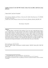
Author's personal copyA. Kaeck, C. Alexander / International Review of Financial Analysis 28 (2013) 46–5655100Level model, b = 0.5, Jump Distribution: exp100Log model, b = 0, Jump Distribution: normal80806060404020200Aug Sep Oct Nov0Aug Sep Oct Nov100Level model, b = 1, Jump Distribution: exp100Log model, b = 1, Jump Distribution: exp80806060404020200Aug Sep Oct Nov0Aug Sep Oct Nov100Log model, SVV, Jump Distribution: no100Log model, SVV, Jump Distribution: normal80806060404020200Aug Sep Oct Nov0Aug Sep Oct NovFig. 4. Simulated VIX 2008. This figure depicts the true evolution of the VIX during the beginning of the banking crisis in 2008. In addition, we plot 95%, 99% and 99.9% percentiles.that they cover rare and extreme events. There is also strong statisticalevidence in favor of time-varying jump intensities in these models.However since one-factor models are misspecified, it is likely that resultsfor these models are distorted. Our simulation experiments showthat the absolute benefit from the addition of jumps to one-factormodels can be fairly small.The only one-factor model that can explain a multitude of facets ofthe VIX is the non-affine log model. A yet more promising approach tocapturing the extreme behavior of the VIX is the inclusion of a stochastic,mean-reverting variance process. This model passes all the specificationhurdles and yields superior results in our scenario analysis. It is also appealingbecause jumps are rare and extreme events, which only occuron days that can be linked to major political or financial news.ReferencesBayarri, M., & Berger, J. (2000). P-values for composite null models. Journal of the AmericanStatistical Association, 95, 1127–1142.Becker, R., Clements, A., & McClelland, A. (2009). The jump component of S&P 500 volatilityand the VIX index. Journal of Banking and Finance, 33(6), 1033–1038.Britten-Jones, M., & Neuberger, A. (2000). Option prices, implied price processes, andstochastic volatility. Journal of Finance, 55(2), 839–866.Broadie, M., Chernov, M., & Johannes, M. (2007). Model specification and risk premia:Evidence from futures options. Journal of Finance, 62(3), 1453–1490.Carr, P., & Wu, L. (2006). A tale of two indices. Journal of Derivatives, 13(3), 13–29.Chernov, M., Gallant, A., Ghysels, E., & Tauchen, G. (2003). Alternative models for stockprice dynamics. Journal of Econometrics, 116(1–2), 225–257.Chourdakis, K., & Dotsis, G. (2011). Maximum likelihood estimation of non-affine volatilityprocesses. Journal of Empirical Finance, 18(3), 533–545.Christoffersen, P., Jacobs, K., & Mimouni, K. (2010). Volatility dynamics for the S&P 500:Evidence from realized volatility, daily returns, and option prices. Review of FinancialStudies, 23(8), 3141–3189.Detemple, J., & Osakwe, C. (2000). The valuation of volatility options. European FinanceReview, 4(1), 21–50.Dotsis, G., Psychoyios, D., & Skiadopoulos, G. (2007). An empirical comparison ofcontinuous-time models of implied volatility indices. Journal of Banking and Finance,31(12), 3584–3603.Duan, J. -C., & Yeh, C. -Y. (2010). Jump and volatility risk premiums implied by VIX.Journal of Economic Dynamics and Control, 34(11), 2232–2244.Eraker, B. (2001). MCMC analysis of diffusion models with application to finance. Journalof Business & Economic Statistics, 19(2), 177–191.Eraker, B., Johannes, M., & Polson, N. (2003). The impact of jumps in volatility andreturns. Journal of Finance, 53(3), 1269–1300.Gelman, A., Meng, X. -L., & Stern, H. (1996). Posterior predictive assessment of modelfitness via realized discrepancies. Statistica Sinica, 6, 733–807.Geman, S., & Geman, G. (1984). Stochastic relaxation, Gibbs distributions, and theBayesian restoration of images. IEEE Transactions on Pattern Analysis and MachineIntelligence, 6, 721–741.Grunbichler, A., & Longstaff, F. (1996). Valuing futures and options on volatility. Journalof Banking & Finance, 20(6), 985–1001.Hagan, P., Kumar, D., Lesniewski, A., & Woodward, D. (2002). Managing smile risk.Wilmott Magazine, 1, 84–108.Hull, J., & White, A. (1987). The pricing of options on assets with stochastic volatilities.Journal of Finance, 42(2), 281–300.Jacquier, E., Polson, N., & Rossi, P. (1994). Bayesian analysis of stochastic volatilitymodels. Journal of Business & Economic Statistics, 12(4), 371–389.Jiang, G., & Tian, Y. (2005). The model-free implied volatility and its information content.Review of Financial Studies, 18(4), 1305–1342.Jiang, G., & Tian, Y. (2007). Extracting model-free volatility from option prices: An examinationof the VIX index. Journal of Derivatives, 14(3), 35–60.Jones, C. (1998). Bayesian estimation of continuous-time finance models. UnpublishedWorking Paper, University of Rochester.Jones, C. (2003). The dynamics of stochastic volatility: Evidence from underlying andoptions markets. Journal of Econometrics, 116, 181–224.

Author's personal copy56 A. Kaeck, C. Alexander / International Review of Financial Analysis 28 (2013) 46–56Kaeck, A., & Alexander, C. (in press). Stochastic volatility jump-diffusions for European equityindex dynamics. European Financial Management. http://dx.doi.org/10.1111/j.1468-036X.2011.00613.x.Konstantinidi, E., Skiadopoulos, G., & Tzagkaraki, E. (2008). Can the evolution ofimplied volatility be forecasted? Evidence from European and US implied volatilityindices. Journal of Banking and Finance, 32(11), 2401–2411.Mencia, J., & Sentana, E. (in press). Valuation of VIX derivatives. Journal of FinancialEconomics. http://dx.doi.org/10.1016/j.jfineco.2012.12.003i.Meng, X. (1994). Posterior predictive p-values. The Annals of Statistics, 22, 1142–1160.Psychoyios, D., Dotsis, G., & Markellos, R. (2010). A jump diffusion model for VIX volatilityoptions and futures. Review of Quantitative Finance and Accounting, 35(3), 245–269.Robert, C., & Casella, G. (2004). Monte Carlo statistical methods. Springer.Rubin, D. (1984). Bayesianly justifiable and relevant frequency calculations for the appliedstatistician. The Annals of Statistics, 12, 1151–1172.Sepp, A. (2008). Pricing options on realized variance in the Heston model with jumpsin returns and volatility. Journal of Computational Finance, 11(4), 33–70.Whaley, R. (1993). Derivatives on market volatility: Hedging tools long overdue. Journalof Derivatives, 1, 71–84.Wu, L. (2011). Variance dynamics: Joint evidence from options and high-frequencyreturns. Journal of Econometrics, 160(1), 280–287.Zhang, J., & Zhu, Y. (2006). VIX futures. The Journal of Futures Markets, 26(6), 521–531.Zhu, S. -P., & Lian, G. -H. (2012). An analytical formula for VIX futures and its applications.The Journal of Futures Markets, 32(2), 166–190.