Feature dimensionality reduction for partial - Berkeley Expert ...

More documents

Recommendations

Info

with different PD sources, thus can be used as features for PD identification orclassification.C) Features from “classification map”. PD pulses are different in wave shape dependingon the location and nature of the underlying defect that generates PD. One way to capture2the different wave shapes is to use so-called “equivalent time-length”, T , and2“equivalent bandwidth”, W [Contin et al (2000)].2 2In the T − W plane (also called the “classification map” by [Contin et al (2000)]), eachPD pulse is presented as a point and each sequence of PD pulses, which are similar in2 2shape, fall into a well-defined area (cluster) in the T − W plane. The location and shape2 2of the clusters in the T − W plane differ corresponding to different PD sources [Continet al (2000 & 2002)]. In this paper, characteristics of the clusters are extracted throughstatistical analysis and used as features for classification purpose. The features extracted22include overall mean, means and standard deviations in both T and W directions,respectively, 1 st through 4 th 22orders of moments of distributions in both T and Wdirections, respectively, direction of the 1 st eigenvector of the cluster, and ratio of the firsttwo eigenvalues of the cluster.D) Features from spectrum analysis. Frequency spectrum of a PD pulse indicatesfrequency components of the PD pulse. Thus the shape or distribution of frequencyspectra should be correlated with different PD sources. In this paper, the first 3frequencies corresponding to the highest three magnitudes, the three highest magnitudesthemselves, the difference between the three frequencies, and the difference between thethree magnitudes are used as features.E) Features from raw PD signals. They are the maximum and minimum peaks of PDpulses, mean and standard deviation of peaks of PD pulses, inception voltage, and PDrate.The five feature extraction methods yield 86 features in total. Including the temperatureand humidity measurements, we have 88 features for each of the 596 data samples, whichwe can use for feature transformation study.4. Classification results: PD diagnosis is a classification problem where the extractedfeatures from PD measurements are the inputs and the sources of PD or condition statusof the wire monitored are the class targets. There are a great number of classifiersavailable, ranging from traditional statistical methods to more modern methods (such asneural network classifiers and support vector machines (SVMs)). To study theeffectiveness of feature transformation on improving classification performance of PDdiagnostic systems, in this paper, we use support vector machines as the classifier fordiagnosing aircraft wiring faults. SVMs are a recently developed learning systemoriginated from the statistical learning theory [Vapnik (1995)]. One distinction betweenSVMs and many other learning systems is that its decision surface is an optimalhyperplane in a high dimensional feature space. The optimal hyperplane ismathematically found by solving a properly formed convex quadratic problem with
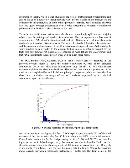
optimization theory, which is well studied in the field of mathematical programming andcan be solved in a relatively straightforward way. For the classification problem we areconcerned in this paper, two of these unique properties, namely, better handling of sparsedata and good average performance over a wide spectrum of different classificationproblems make SVM classifiers a better choice here.To evaluate classification performance, the data set is randomly split into two disjointsubsets: one for training and another for evaluation. Also, to improve the robustness ofevaluation, the SVM classifier is trained and evaluated 10 times and each time the data israndomly split into two disjoint subsets. The mean, the standard deviation, the minimum,and the maximum of accuracies of the 10 evaluations are reported here. Additionally, 1-sigma random noise is added to the original feature values in order to account for thefacts that only limited PD examples are obtained in well-defined lab environment andthat PD measurements in real aircraft wires will be much more noisy.The PCA results: First, we apply PCA to the 88-feature data set described in theprevious section. Figure 2 shows the variance explained by each of the principalcomponents (PCs). For illustration convenience, only the first 30 PCs with largestvariance explained are shown in the figure. The vertical bars show the percentage of thetotal variance explained by each individual principal component, while the line with dotsshows the cumulative percentage of the total variance explained by all principalcomponents up to the specific one.Figure 2: Variance explained by the first 30 principal componentsAs we can see from the figure, the first 10 PCs explain approximately 60% of the totalvariance of the data whereas the first 30 PCs explain about 80% of the total variance.Classification accuracies for the designs using the first 3, 10, and 30 PCs as classifierinputs are shown in Table I, respectively. For comparison, also included in Table I are theclassification accuracies for the design with all 88 features extracted from the PD signalsas its inputs. From Table I, we can see that using only the first 3 PCs as the classifierinputs already provides a reasonable performance – better than that from using all 88
Page 2: activities, generally known as “P
Page 5: sequences are used for designing th
Page 9 and 10: performance for the PD diagnosis pr

Feature dimensionality reduction for partial - Berkeley Expert ...

Create successful ePaper yourself

Delete template?

Save as template?