Diagnostic Information Fusion for Manufacturing Processes

Proceedings of the 2nd International Conference on Information Fusion, Fusion ’99, vol. 1, pp. 331-336, 1999
Diagnostic Information Fusion for Manufacturing Processes
Kai Goebel & Vivek Badami
GE Corporate R&D
Niskayuna, NY 12309
goebelk@crd.ge.com; badami@crd.ge.com
Amitha Perera
Rensselear Polytechnic Institute
Troy, NY 12380
perera@cs.rpi.edu
Abstract - This paper addresses diagnostic
information fusion for situations where several
diagnostic tools are used to estimate a single system
state. These estimates will always disagree to some
extent and it is the task of the fusion module to
provide an estimate which is more reliable than the
best of the diagnostic tools. To that end, a fusion
process was developed which performs a weighted
average of individual tools using confidence values
assigned dynamically to the individual diagnostic
tools. These confidence values are derived from
validation curves which are designed using individual
a priori tool information and which are centered about
the previous system estimate. In a further step, the
fusion output is smoothed leading to additional
performance improvement. In experiments, data were
gathered from a high speed milling machine and fed
through several developed diagnostic tools.
Key words: fusion, information fusion, diagnosis,
soft computing, fuzzy fusion.
of above mentioned techniques and other soft
computing principles for diagnostics and prognostics
are given in Bonissone and Goebel [8]. In a similar
spirit, fusion techniques combine different methods to
overcome shortcomings of individual tools. This
paper proposes one fusion method based on fuzzy
validation gates.
Diagnostic Fusion via Validation Gates
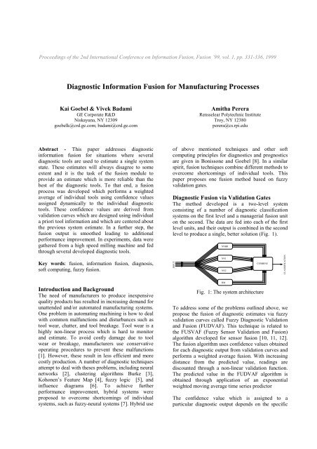
The method developed is a two-level system
consisting of a number of diagnostic classification
systems on the first level and a managerial fusion unit
on the second. The data are fed into each of the first
level units, and their output is combined in the second
level to produce a single, better solution (Fig. 1).
INPUT
NNBR
NN1
NN2
COMBINE
CLASSIFICATION
Introduction and Background
The need of manufacturers to produce inexpensive
quality products has resulted in increasing demand for
unattended and/or automated manufacturing systems.
One problem in automating machining is how to deal
with common malfunctions and disturbances such as
tool wear, chatter, and tool breakage. Tool wear is a
highly non-linear process which is hard to monitor
and estimate. To avoid costly damage due to tool
wear or breakage, manufacturers use conservative
operating procedures to prevent these malfunctions
[1]. However, these result in less efficient and more
costly production. A number of diagnostic techniques
attempt to deal with theses problems, including neural
networks [2], clustering algorithms Burke [3],
Kohonen’s Feature Map [4], fuzzy logic [5], and
influence diagrams [6]. To achieve further
performance improvement, hybrid systems were
proposed to overcome shortcomings of individual
systems, such as fuzzy-neural systems [7]. Hybrid use
RM
Fig. 1: The system architecture
To address some of the problems outlined above, we
propose the fusion of diagnostic estimates via fuzzy
validation curves called Fuzzy Diagnostic Validation
and Fusion (FUDVAF). This technique is related to
the FUSVAF (Fuzzy Sensor Validation and Fusion)
algorithm developed for sensor fusion [10, 11, 12].
The fusion algorithm uses confidence values obtained
for each diagnostic output from validation curves and
performs a weighted average fusion. With increasing
distance from the predicted value, readings are
discounted through a non-linear validation function.
The predicted value in the FUDVAF algorithm is
obtained through application of an exponential
weighted moving average time series predictor
The confidence value which is assigned to a
particular diagnostic output depends on the specific

tool characteristics, the predicted value, and the
physical limitations of the diagnostic value. The
assignment takes place in a validation region which
assigns a maximum value to readings which coincide
with the predicted value. The curve is dependent on
the sensor behavior. Generally, this is a nonsymmetric
curve which is wider around the maximum
value if the diagnostic tool is more reliable and
narrower if it is less reliable.
A choice for validation curves σ(z) could be a bell
curve of the form
( )
σ d
t
= 1−
e
−
( dt
−d
)
at
m
2
where
m is a scaling parameter
a i is the tool accuracy
d i is the diagnosis of tool i
d is the estimated diagnosis
A validation gate is shown in Fig. 2.
confidence
σ 1
σ 3
σ 2
d 2 (k) d 3 (k)
d(k-1)
d 1 (k)
dt diagnostic output
σi confidence values
d ( k − 1)
fused value
diagnostic
output
Fig. 2: Validation gate for the assignment of
confidence values
The fusion is performed through a weighted average
of confidence values and diagnostic output. The sum
of the confidence values times the measurements
rewards measurements closest to the old fused value
the most, depending on the validation curve which
expresses a trust in the operation of each diagnostic
tool through the design of its shape. Measurements
further away are discounted. The operative equation
in the FUDVAF algorithm is
d
n
d σ
t
t
f = = 1
n
t=
1
σ
( d )
t
( d )
t
where
df: fused value
dt: diagnostic output of tool t
σ: confidence values
Note that if all diagnostic outputs lie on one side of
the predicted value, the fused value will also be
pulled to the same side. This ensures that evidence
from the diagnostic tools is closely followed yet
discounted the further it gets away from the predicted
value.
We used a time series filter to further improve the
result of the system using the standard EWMA
predictor of the form
σ t d t
d
( k) d
t
= ( k − 1) α + ( 1−α
)
σ
where
t
α is the smoothing parameter; α=0.1
t
Experimental Setup
A milling machine under various operating conditions
was selected as the manufacturing environment. In
particular, tool wear was investigated in a regular cut
as well as entry cut and exit cut. Data sampled by
three different types of sensors (acoustic emission
sensor, vibration sensor, motor current sensor) were
used to determine the state of wear of the tool. As the
wear measure, flank wear VB (the distance from the
cutting edge to the end of the abrasive wear on the
flank face of the tool) was chosen. The flank wear
was observed during the experiments by taking the
insert out of the tool and physically measuring the
wear. The setup of the experiment is as depicted in
Fig. 3. The basic setup encompasses the spindle and
the table of the Matsuura machining center MC-
510V. An acoustic emission sensor and a vibration
sensor are each mounted to the table and the spindle
of the machining center. The signals from all sensors
are amplified and filtered, then fed through two RMS
before they enter the computer for data acquisition.
The signal from a spindle motor current sensor is fed
into the computer without further processing. Data
are categorized into four classes and are
approximated by fuzzy membership functions (no
wear, little wear, medium wear, high wear) shown in
Fig. 6.

ACOUSTIC EMISSION
SENSOR SPINDLE
ACOUSTIC EMISSION
SENSOR TABLE
PREAMPLIFIER
PREAMPLIFIER
RMS
RMS
1.2
1
The output
Original
Smoothed
VIBRATION SENSOR
SPINDLE
CHARGE AMPLIFIER
LP/HP FILTER
RMS
COMPUTER
0.8
VIBRATION SENSOR
TABLE
SPINDLE MOTOR
CURRENT SENSOR
CHARGE AMPLIFIER
LP/HP FILTER
RMS
Degree of wear
0.6
0.4
RECORDER
Fig. 3: Experimental setup
0.2
0
Input data transformations
Before being used, the following transformations
were applied to the data:
1.) The data was smoothed by averaging using a
window of 50 points, and then the sample size was
reduced by sampling the resulting data set at 50 point
intervals. 2.) Each input and the output data was
normalized to lie between 0 and 1. 3.) Since the
output variable was sampled at much larger intervals
than the input variables, and since it represents tool
wear, the output data was further smoothed by fitting
a 3rd order polynomial.
Fig. 4 and Fig. 5 show the normalized and smoothed
input and output data. The output
data was categorized into four classes using fuzzy
membership functions.
−0.2
0 200 400 600 800 1000 1200 1400
Sample number
Fig. 5: Ouput data
Degree of membership
1
0.9
0.8
0.7
0.6
0.5
0.4
0.3
0.2
Membership functions for the output classes
1
0.9
0.8
0.7
0.6
0.5
0.4
0.3
0.2
0.1
The inputs
0
0 200 400 600 800 1000 1200 1400
Sample number
Fig. 4: Input data
0.1
0
0 0.1 0.2 0.3 0.4 0.5 0.6 0.7 0.8 0.9 1
Degree of wear
Fig. 6: Membership functions
Diagnostic tools employed
Nearest neighbor classifier (NNBR): The first
subsystem uses a nearest neighbor scheme for
classifying the data. The case base consists of a set of
sensor readings and the associated unclassified wear
value. Given an input, the k nearest data points are
determined and the associated wear values are
averaged. This average is then used to compute the
membership degree for each of the four classes.
Neural network (NN1): The second subsystem is a
neural network that was trained on binary classes.
That is, the target values were 0 and 1 vectors
determined by the maximum membership value over
the four classes.
Neural network (NN2): The third subsystem is also a
neural network, but this was trained to learn the
membership values themselves, as opposed to the
classes.
Fuzzy inference system (RM): The fourth subsystem
is a fuzzy inference system implemented using a
relation matrix.

Architecture
As shown in Fig. 1, the input to the first level of the
system are the measured features. The output consists
of four values indicating the degree of membership
for each of the four output classes. We chose this
approach over an approach where the first level
subsystem generates a crisp class (from 1 to 4)
because this approach gives more flexibility and
information to the second level system. This is in
response to the need recognized after development of
the neural-fuzzy diagnostic tool [9] which attempted
to segment the data into five crisp classes. In the
approach chosen here, the membership approach
allows a softer classification. The second level system
then combines the results of the first level systems
and classifies the input into a single class. We will be
focusing in this paper on the fusion task and evaluate
performance based on the fused membership values.
One basic problem in averaging techniques or
majority voting techniques is the danger of ending up
with a system which performed worth than the best
individual tool because the poor estimates drag down
the better estimate. One potential solution is to weigh
the tools according to their performance which must
be known beforehand. The FUDVAF tries to perform
this task. Stand alone tests were performed to
establish the accuracy of the individual diagnostic
tools which are shown in Table 1.
Table 1: Classification rates
System Rate (%)
Nearest neighbor (NNBR) 96.8
Neural network 1 (NN1) 80.6
Neural network 2 (NN2) 86.7
Relational matrix (RM) 81.0
1
0.9
0.8
0.7
0.6
0.5
0.4
0.3
0.2
0.1
0
0 200 400 600 800 1000 1200 1400
1
0.9
0.8
0.7
0.6
0.5
0.4
0.3
0.2
0.1
Neural network 1
Fig. 8: Output NN1
0
0 200 400 600 800 1000 1200 1400
1
Neural network 2
Fig. 9: Output NN2
Relational matrix
1
Nearest neighbour
0.9
0.8
0.9
0.7
0.8
0.6
0.7
0.5
0.6
0.4
0.5
0.3
0.4
0.2
0.3
0.1
0.2
0.1
0
0 200 400 600 800 1000 1200 1400
Fig. 7: Output NNBR
0
0 200 400 600 800 1000 1200 1400
Fig. 10: Output RBS
Fig. 7 to Fig. 10 depict the performance of the
individual systems. The solid lines show the true
membership values for the data. The crosses indicate
the membership values generated by the system when

the system disagrees on the classification. Thus, the
crosses are an indication of the area(s) in which the
system has difficulty in deciding on a class. Fig. 7
shows that NNBR has classification errors only near
the cross-over points of the membership functions.
These are areas where classification errors are
expected, because a small change in the membership
value results in an incorrect classification. Even at
these points, however, NNBR membership values are
very close to the true membership values. The success
of this system is due to the continuous nature of the
wear measure, and the averaging technique used in
the nearest neighbor classification. The other systems
are not as successful, and the membership values
output do not approximate the true values to the
degree that NNBR does.
The high success rate of one tool means that if it were
used as part of the majority fusion, the performance
degrades somewhat. This is to be expected, because
the votes of the poor performers will sometimes out
vote the correct one. The problem is greater with
increasing number of classification regions, as there
will be cases when each system will generate a
different class, and the majority voting system will
then pick one randomly.
Results
The fusion using assignment of confidence values
provides a means to integrate a priori information
about individual tool performance. This is
accomplished by designing the validation curves of a
better tool wider than the curves of the tools with
worse performance. The fused performance improves
the already very good performance of the NNBR tool
from 96.8% to 99.1% correct classification with
α=0.1 and m=0.1. Fig. 11 shows the result of the
fused system where the membership functions no
wear, little wear, medium wear, and high wear were
estimated.
Fig. 11: Fused system output
Summary and Final Remarks
The use of the FUDVAF algorithm provides a means
to improve performance of individual diagnostic
tools. In experiments with data from a milling
machine, we show how the FUDVAF can be used for
extant systems. Much of performance improvement
appears to be due to the smoothing and an increase of
performance might also be expected when the
smoothing is applied to the best tool alone.
Future research should address how to improve fine
tuning of the validation curve parameters, depending
on operating conditions and sensor history. This can
be accomplished through machine learning
techniques similar to the approach used for the
FUSVAF algorithm [11]. Also helpful might be
knowledge about locally changing diagnostic tool
performance. Such local characteristics could be
utilized in designing the validation curves in a
dynamic manner by changing the width accordingly.
Generally, it is desirable to maintain maximum
independence of the diagnostic tools in the sense that
tools which exhibit poor performance in certain
operating conditions are matched with tools
exhibiting better conditions there. This may, of
course, not always be possible due to the limitations
of observable conditions and shortcomings of the
diagnostic tools because often times (and in this
approach here), all sensor values are made available
to all diagnostic tools.
Acknowledgements

The authors thank Prof. A. Agogino for her support
and advice; Prof. D. Dornfeld and Prof. Tomizuka
(all of UC Berkeley) for making available equipment;
and Andrzej Sokolowski and Piotr Dworak for
helping with the experiments.
References
[1] Rangwala, S.S., and D.Dornfeld “Learning and
Optimization of Machining Operations Using
Computing Abilities of Neural Networks”, IEEE
Transactions of Systems, Man & Cybernetics,
Vol. 19, No. 2, March/April 1989.
[2] Rangwala, S.S. “Machining Process
Characterization and Intelligent Tool Condition
Monitoring Using Acoustic Emission Signal
Emission Signal Analysis”, PhD thesis, UC
Berkeley, 1988.
[3] Burke, L. I. “Automated Identification of Tool
Wear States in Machining Processes: An
Application of Self Organizing Neural Networks,”
PhD thesis, UC Berkeley, 1989.
[4] Leem, C.S. “Input Feature Scaling Algorithm for
Competitive Learning Based Cognitive Modeling
with Two Applications”, PhD thesis, UC
Berkeley, 1992.
[5] Fei, J., and I.S. Jawahir “A Fuzzy Classification
Technique for Predictive Assessment of Chip
Breakability in Intelligent Machining Systems”,
Proc. IEEE Joint Conference on Fuzzy Logic and
Neural Networks, San Francisco, 1993.
[6] Agogino, A. M., and K. Ramamurthi “Real Time
Influence Diagrams for Monitoring and
Controlling Mechanical Systems,“ Influence
Diagrams, Belief Nets and Decision Analysis, Ed.:
Oliver, R. M., and J.O. Smith. J.R. Wiley & Sons,
Ltd., 1990.
[7] Goebel, K., and P.K. Wright “Monitoring and
Diagnosing Manufacturing Processes Using a
Hybrid Architecture with Neural Networks and
Fuzzy Logic”, EUFIT, Proceedings, Vol. 2,
Aachen, Germany, 1993.
[8] Bonissone, P., and Goebel, K., “Soft Comuting
Principles for Diagnostics”, working notes of the
AAAI Spring symposium, Palo Alto, 1999.
[9] Goebel, K., Wood, W., Agogino, A., and Jain, P.,
“Comparing a Neural-Fuzzy Scheme and a
Probabilistic Neural Network for Monitoring of
Manufacturing Processes”, Working Notes of the
AAAI Spring Symposium, 1994.
[10] Agogino, A., Alag, S., and Goebel, K.,
Proceedings of the 1995 Annual Meeting of ITS
America A Framework for Intelligent Sensor
Validation, Sensor Fusion, and Supervisory
Control of Automated Vehicles in IVHS, 1995.
[11] Goebel, K., Management of Uncertainty for
Sensor Validation, Sensor Fusion, and Diagnosis
Using Soft Computing Techniques Ph.D. Thesis,
University of California at Berkeley, 1996.
[12] Goebel, K., and Agogino, A.M., Proceedings of
the 29th ISATA An Architecture for Fuzzy Sensor
Validation and Fusion for Vehicle Following in
Automated Highways, 1996.