Diagnostic Information Fusion for Manufacturing Processes

More documents

Recommendations

Info

Architecture As shown in Fig. 1, the input to the first level of the system are the measured features. The output consists of four values indicating the degree of membership for each of the four output classes. We chose this approach over an approach where the first level subsystem generates a crisp class (from 1 to 4) because this approach gives more flexibility and information to the second level system. This is in response to the need recognized after development of the neural-fuzzy diagnostic tool [9] which attempted to segment the data into five crisp classes. In the approach chosen here, the membership approach allows a softer classification. The second level system then combines the results of the first level systems and classifies the input into a single class. We will be focusing in this paper on the fusion task and evaluate performance based on the fused membership values. One basic problem in averaging techniques or majority voting techniques is the danger of ending up with a system which performed worth than the best individual tool because the poor estimates drag down the better estimate. One potential solution is to weigh the tools according to their performance which must be known beforehand. The FUDVAF tries to perform this task. Stand alone tests were performed to establish the accuracy of the individual diagnostic tools which are shown in Table 1. 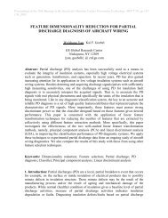Table 1: Classification rates System Rate (%) Nearest neighbor (NNBR) 96.8 Neural network 1 (NN1) 80.6 Neural network 2 (NN2) 86.7 Relational matrix (RM) 81.0 1 0.9 0.8 0.7 0.6 0.5 0.4 0.3 0.2 0.1 0 0 200 400 600 800 1000 1200 1400 1 0.9 0.8 0.7 0.6 0.5 0.4 0.3 0.2 0.1 Neural network 1 Fig. 8: Output NN1 0 0 200 400 600 800 1000 1200 1400 1 Neural network 2 Fig. 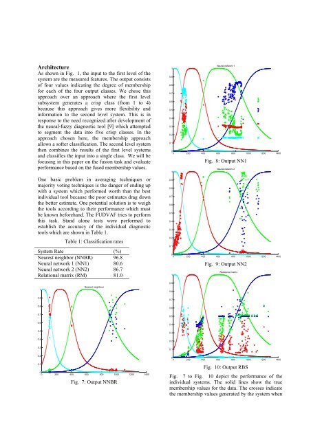9: Output NN2 Relational matrix 1 Nearest neighbour 0.9 0.8 0.9 0.7 0.8 0.6 0.7 0.5 0.6 0.4 0.5 0.3 0.4 0.2 0.3 0.1 0.2 0.1 0 0 200 400 600 800 1000 1200 1400 Fig. 7: Output NNBR 0 0 200 400 600 800 1000 1200 1400 Fig. 10: Output RBS Fig. 7 to Fig. 10 depict the performance of the individual systems. The solid lines show the true membership values for the data. The crosses indicate the membership values generated by the system when
the system disagrees on the classification. Thus, the crosses are an indication of the area(s) in which the system has difficulty in deciding on a class. Fig. 7 shows that NNBR has classification errors only near the cross-over points of the membership functions. These are areas where classification errors are expected, because a small change in the membership value results in an incorrect classification. Even at these points, however, NNBR membership values are very close to the true membership values. The success of this system is due to the continuous nature of the wear measure, and the averaging technique used in the nearest neighbor classification. The other systems are not as successful, and the membership values output do not approximate the true values to the degree that NNBR does. The high success rate of one tool means that if it were used as part of the majority fusion, the performance degrades somewhat. This is to be expected, because the votes of the poor performers will sometimes out vote the correct one. The problem is greater with increasing number of classification regions, as there will be cases when each system will generate a different class, and the majority voting system will then pick one randomly. Results The fusion using assignment of confidence values provides a means to integrate a priori information about individual tool performance. This is accomplished by designing the validation curves of a better tool wider than the curves of the tools with worse performance. The fused performance improves the already very good performance of the NNBR tool from 96.8% to 99.1% correct classification with α=0.1 and m=0.1. Fig. 11 shows the result of the fused system where the membership functions no wear, little wear, medium wear, and high wear were estimated. Fig. 11: Fused system output Summary and Final Remarks The use of the FUDVAF algorithm provides a means to improve performance of individual diagnostic tools. In experiments with data from a milling machine, we show how the FUDVAF can be used for extant systems. Much of performance improvement appears to be due to the smoothing and an increase of performance might also be expected when the smoothing is applied to the best tool alone. Future research should address how to improve fine tuning of the validation curve parameters, depending on operating conditions and sensor history. This can be accomplished through machine learning techniques similar to the approach used for the FUSVAF algorithm [11]. Also helpful might be knowledge about locally changing diagnostic tool performance. Such local characteristics could be utilized in designing the validation curves in a dynamic manner by changing the width accordingly. Generally, it is desirable to maintain maximum independence of the diagnostic tools in the sense that tools which exhibit poor performance in certain operating conditions are matched with tools exhibiting better conditions there. This may, of course, not always be possible due to the limitations of observable conditions and shortcomings of the diagnostic tools because often times (and in this approach here), all sensor values are made available to all diagnostic tools. Acknowledgements
Page 1 and 2: Proceedings of the 2nd Internationa
Page 3: ACOUSTIC EMISSION SENSOR SPINDLE AC

Diagnostic Information Fusion for Manufacturing Processes

You also want an ePaper? Increase the reach of your titles

Delete template?

Save as template?