Diagnostic Information Fusion for Manufacturing Processes

tool characteristics, the predicted value, and the
physical limitations of the diagnostic value. The
assignment takes place in a validation region which
assigns a maximum value to readings which coincide
with the predicted value. The curve is dependent on
the sensor behavior. Generally, this is a nonsymmetric
curve which is wider around the maximum
value if the diagnostic tool is more reliable and
narrower if it is less reliable.
A choice for validation curves σ(z) could be a bell
curve of the form
( )
σ d
t
= 1−
e
−
( dt
−d
)
at
m
2
where
m is a scaling parameter
a i is the tool accuracy
d i is the diagnosis of tool i
d is the estimated diagnosis
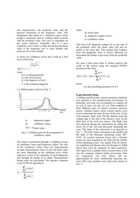
A validation gate is shown in Fig. 2.
confidence
σ 1
σ 3
σ 2
d 2 (k) d 3 (k)
d(k-1)
d 1 (k)
dt diagnostic output
σi confidence values
d ( k − 1)
fused value
diagnostic
output
Fig. 2: Validation gate for the assignment of
confidence values
The fusion is performed through a weighted average
of confidence values and diagnostic output. The sum
of the confidence values times the measurements
rewards measurements closest to the old fused value
the most, depending on the validation curve which
expresses a trust in the operation of each diagnostic
tool through the design of its shape. Measurements
further away are discounted. The operative equation
in the FUDVAF algorithm is
d
n
d σ
t
t
f = = 1
n
t=
1
σ
( d )
t
( d )
t
where
df: fused value
dt: diagnostic output of tool t
σ: confidence values
Note that if all diagnostic outputs lie on one side of
the predicted value, the fused value will also be
pulled to the same side. This ensures that evidence
from the diagnostic tools is closely followed yet
discounted the further it gets away from the predicted
value.
We used a time series filter to further improve the
result of the system using the standard EWMA
predictor of the form
σ t d t
d
( k) d
t
= ( k − 1) α + ( 1−α
)
σ
where
t
α is the smoothing parameter; α=0.1
t
Experimental Setup
A milling machine under various operating conditions
was selected as the manufacturing environment. In
particular, tool wear was investigated in a regular cut
as well as entry cut and exit cut. Data sampled by
three different types of sensors (acoustic emission
sensor, vibration sensor, motor current sensor) were
used to determine the state of wear of the tool. As the
wear measure, flank wear VB (the distance from the
cutting edge to the end of the abrasive wear on the
flank face of the tool) was chosen. The flank wear
was observed during the experiments by taking the
insert out of the tool and physically measuring the
wear. The setup of the experiment is as depicted in
Fig. 3. The basic setup encompasses the spindle and
the table of the Matsuura machining center MC-
510V. An acoustic emission sensor and a vibration
sensor are each mounted to the table and the spindle
of the machining center. The signals from all sensors
are amplified and filtered, then fed through two RMS
before they enter the computer for data acquisition.
The signal from a spindle motor current sensor is fed
into the computer without further processing. Data
are categorized into four classes and are
approximated by fuzzy membership functions (no
wear, little wear, medium wear, high wear) shown in
Fig. 6.