GRAIL: Scalable Reachability Index for Large Graphs ∗ - CiteSeerX

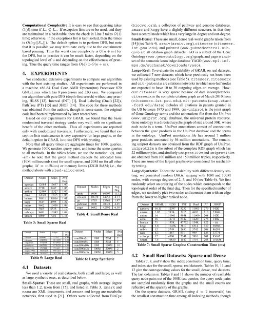
Computational Complexity: It is easy to see that querying takesO(d) time if L v ⊈ L u. If exception lists are to be used, and theyare maintained in a hash table, then the check in Line 3 takesO(1)time; otherwise, if the exceptions list is kept sorted, then the timesis O(log(|E u|)). The default option is to perform DFS, but notethat it is possible we may terminate early due to the containmentbased pruning. Thus the worst case complexity is O(n + m) forthe DFS, but in practice it can be much faster, depending on thetopological level of u and depending on the effectiveness of pruning.Thus the query time ranges fromO(d) toO(n+m).4. EXPERIMENTSWe conducted extensive experiments to compare our algorithmwith the best existing studies. All experiments are performed ina machine x86 64 Dual Core AMD Opteron(tm) Processor 870GNU/Linux which has 8 processors and 32G ram. We comparedour algorithm with pure DFS (depth-first search) without any pruning,HLSS [12], Interval (INT) [1], Dual Labeling (Dual) [22]),PathTree (PT) [15] and 3HOP [14]. The code for these methodswas obtained from the authors, though in some cases, the originalcode had been reimplemented by later researchers.Based on our experiments for GRAIL we found that the basicrandomized traversal strategy works very well, with no significantbenefit of the other methods. Thus all experiments are reportedonly with randomized traversals. Furthermore, we found that exceptionlists maintenance is very expensive for large graphs, so thedefault option in GRAIL is to use DFS with pruning.Note that all query times are aggregate times for 100K queries.We generate 100K random query pairs, and issue the same queriesto all methods. In the tables below, we use the notation –(t), and–(m), to note that the given method exceeds the allocated time(10M milliseconds (ms) for small sparse, and 20M ms for all othergraphs; M ≡ million) or memory limits (32GB RAM; i.e., themethod aborts with a bad-alloc error).Dataset Nodes Edges AvgDegagrocyc 12684 13657 1.07amaze 3710 3947 1.06anthra 12499 13327 1.07ecoo 12620 13575 1.08human 38811 39816 1.01kegg 3617 4395 1.22mtbrv 9602 10438 1.09nasa 5605 6538 1.17vchocyc 9491 10345 1.09xmark 6080 7051 1.16Table 3: Small Sparse RealDataset Nodes Edges AvgDegciteseer 693947 312282 0.45citeseerx 6540399 15011259 2.30cit-patents 3774768 16518947 4.38go-uniprot 6967956 34770235 4.99uniprot22m 1595444 1595442 1.00uniprot100m 16087295 16087293 1.00uniprot150m 25037600 25037598 1.00Table 5: Large RealDataset Nodes Edges AvgDegarxiv 6000 66707 11.12citeseer 10720 44258 4.13go 6793 13361 1.97pubmed 9000 40028 4.45yago 6642 42392 6.38Table 4: Small Dense RealDataset Nodes Edges AvgDegrand10m2x 10M 20M 2rand10m5x 10M 50M 5rand10m10x 10M 100M 10rand100m2x 100M 200M 2rand100m5x 100M 500M 5Table 6: Large Synthetic4.1 DatasetsWe used a variety of real datasets, both small and large, as wellas large synthetic ones, as described below.Small-Sparse: These are small, real graphs, with average degreeless than 1.2, taken from [15], and listed in Table 3. xmark andnasa are XML documents, and amaze and kegg are metabolicnetworks, first used in [21]. Others were collected from BioCyc(biocyc.org), a collection of pathway and genome databases.amaze and kegg have a slightly different structure, in that theyhave a central node which has a very large in-degree and out-degree.Small-Dense: These are small, dense real-world graphs taken from[14] (see Table 4). arxiv (arxiv.org), citeceer (citeseer.ist.psu.edu), and pubmed (www.pubmedcentral.nih.gov) are all citation graph datasets. GO is a subset of the GeneOntology (www.geneontology.org) graph, and yago is a subsetof the semantic knowledge database YAGO (www.mpi-inf.mpg.de/suchanek/downloads/yago).Large-Real: To evaluate the scalability of GRAIL on real datasets,we collected 7 new datasets which have previously not been beenused by existing methods (see Table 5). citeseer, citeseerxand cit-patents are citations networks in which non-leaf nodesare expected to have 10 to 30 outgoing edges on average. Howeverciteseer is very sparse because of data incompleteness.citeseerx is the complete citation graph as of March 2010 from(citeseerx.ist.psu.edu). cit-patents (snap.stan\-ford.edu/data) includes all citations in patents granted inthe US between 1975 and 1999. go-uniprot is the joint graphof Gene Ontology terms and the annotations file from the UniProt(www.uniprot.org) database, the universal protein resource.Gene ontology is a directed acyclic graph of size around 30K, whereeach node is a term. UniProt annotations consist of connectionsbetween the gene products in the UniProt database and the termsin the ontology. UniProt annotations file has around 7 milliongene products annotated by 56 million annotations. The remaininguniprot datasets are obtained from the RDF graph of UniProt.uniprot22m is the subset of the complete RDF graph which has22 million triples, and similarly uniprot100m and uniprot150mare obtained from 100 million and 150 million triples, respectively.These are some of the largest graphs ever considered for reachabilitytesting.Large-Synthetic: To test the scalability with different density setting,we generated random DAGs, ranging with 10M and 100Mnodes, with average degrees of 2, 5, and 10 (see Table 6). We firstrandomly select an ordering of the nodes which corresponds to thetopological order of the final dag. Then for the specified number ofedges, we randomly pick two nodes and connect them with an edgefrom the lower to higher ranked node.Dataset GRAIL HLSS INT Dual PT 3HOPagrocyc 16.13 12397 5232 11803 279 142Kamaze 3.82 703K 3215 4682 818 2304Kanthra 16 11961 4848 11600 268 142Kecoo 16 12711 5142 12287 276 146Khuman 71 135K 47772 134K 822 – (t)kegg 3.8 1145K 3810 6514 939 3888Kmtbrv 12 3749 2630 3742 208 86291nasa 6.3 1887 811 999 126 33774vchocyc 12 4500 2541 3910 201 85667xmark 7.5 70830 1547 1719 263 151856Table 7: Small Sparse Graphs: Construction Time (ms)4.2 Small Real Datasets: Sparse and DenseTables 7, 8, and 9 show the index construction time, query time,and index size for the small, sparse, real datasets. Tables 10, 11, and12 give the corresponding values for the small, dense, real datasets.The last column in Tables 8 and 11 shows the number of reachablequery node-pairs out of the 100K test queries; the query node-pairsare sampled randomly from the graphs and the small counts arereflective of the sparsity of the graphs.On the sparse datasets, GRAIL (using d = 2 traversals) hasthe smallest construction time among all indexing methods, though