GRAIL: Scalable Reachability Index for Large Graphs ∗ - CiteSeerX

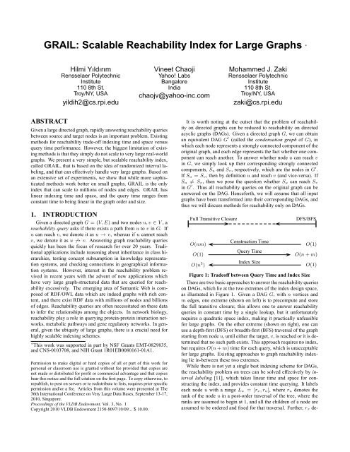
Computational Complexity: It is easy to see that querying takesO(d) time if L v ⊈ L u. If exception lists are to be used, and theyare maintained in a hash table, then the check in Line 3 takesO(1)time; otherwise, if the exceptions list is kept sorted, then the timesis O(log(|E u|)). The default option is to perform DFS, but notethat it is possible we may terminate early due to the containmentbased pruning. Thus the worst case complexity is O(n + m) forthe DFS, but in practice it can be much faster, depending on thetopological level of u and depending on the effectiveness of pruning.Thus the query time ranges fromO(d) toO(n+m).4. EXPERIMENTSWe conducted extensive experiments to compare our algorithmwith the best existing studies. All experiments are performed ina machine x86 64 Dual Core AMD Opteron(tm) Processor 870GNU/Linux which has 8 processors and 32G ram. We comparedour algorithm with pure DFS (depth-first search) without any pruning,HLSS [12], Interval (INT) [1], Dual Labeling (Dual) [22]),PathTree (PT) [15] and 3HOP [14]. The code for these methodswas obtained from the authors, though in some cases, the originalcode had been reimplemented by later researchers.Based on our experiments for GRAIL we found that the basicrandomized traversal strategy works very well, with no significantbenefit of the other methods. Thus all experiments are reportedonly with randomized traversals. Furthermore, we found that exceptionlists maintenance is very expensive for large graphs, so thedefault option in GRAIL is to use DFS with pruning.Note that all query times are aggregate times for 100K queries.We generate 100K random query pairs, and issue the same queriesto all methods. In the tables below, we use the notation –(t), and–(m), to note that the given method exceeds the allocated time(10M milliseconds (ms) for small sparse, and 20M ms for all othergraphs; M ≡ million) or memory limits (32GB RAM; i.e., themethod aborts with a bad-alloc error).Dataset Nodes Edges AvgDegagrocyc 12684 13657 1.07amaze 3710 3947 1.06anthra 12499 13327 1.07ecoo 12620 13575 1.08human 38811 39816 1.01kegg 3617 4395 1.22mtbrv 9602 10438 1.09nasa 5605 6538 1.17vchocyc 9491 10345 1.09xmark 6080 7051 1.16Table 3: Small Sparse RealDataset Nodes Edges AvgDegciteseer 693947 312282 0.45citeseerx 6540399 15011259 2.30cit-patents 3774768 16518947 4.38go-uniprot 6967956 34770235 4.99uniprot22m 1595444 1595442 1.00uniprot100m 16087295 16087293 1.00uniprot150m 25037600 25037598 1.00Table 5: Large RealDataset Nodes Edges AvgDegarxiv 6000 66707 11.12citeseer 10720 44258 4.13go 6793 13361 1.97pubmed 9000 40028 4.45yago 6642 42392 6.38Table 4: Small Dense RealDataset Nodes Edges AvgDegrand10m2x 10M 20M 2rand10m5x 10M 50M 5rand10m10x 10M 100M 10rand100m2x 100M 200M 2rand100m5x 100M 500M 5Table 6: Large Synthetic4.1 DatasetsWe used a variety of real datasets, both small and large, as wellas large synthetic ones, as described below.Small-Sparse: These are small, real graphs, with average degreeless than 1.2, taken from [15], and listed in Table 3. xmark andnasa are XML documents, and amaze and kegg are metabolicnetworks, first used in [21]. Others were collected from BioCyc(biocyc.org), a collection of pathway and genome databases.amaze and kegg have a slightly different structure, in that theyhave a central node which has a very large in-degree and out-degree.Small-Dense: These are small, dense real-world graphs taken from[14] (see Table 4). arxiv (arxiv.org), citeceer (citeseer.ist.psu.edu), and pubmed (www.pubmedcentral.nih.gov) are all citation graph datasets. GO is a subset of the GeneOntology (www.geneontology.org) graph, and yago is a subsetof the semantic knowledge database YAGO (www.mpi-inf.mpg.de/suchanek/downloads/yago).Large-Real: To evaluate the scalability of GRAIL on real datasets,we collected 7 new datasets which have previously not been beenused by existing methods (see Table 5). citeseer, citeseerxand cit-patents are citations networks in which non-leaf nodesare expected to have 10 to 30 outgoing edges on average. Howeverciteseer is very sparse because of data incompleteness.citeseerx is the complete citation graph as of March 2010 from(citeseerx.ist.psu.edu). cit-patents (snap.stan\-ford.edu/data) includes all citations in patents granted inthe US between 1975 and 1999. go-uniprot is the joint graphof Gene Ontology terms and the annotations file from the UniProt(www.uniprot.org) database, the universal protein resource.Gene ontology is a directed acyclic graph of size around 30K, whereeach node is a term. UniProt annotations consist of connectionsbetween the gene products in the UniProt database and the termsin the ontology. UniProt annotations file has around 7 milliongene products annotated by 56 million annotations. The remaininguniprot datasets are obtained from the RDF graph of UniProt.uniprot22m is the subset of the complete RDF graph which has22 million triples, and similarly uniprot100m and uniprot150mare obtained from 100 million and 150 million triples, respectively.These are some of the largest graphs ever considered for reachabilitytesting.Large-Synthetic: To test the scalability with different density setting,we generated random DAGs, ranging with 10M and 100Mnodes, with average degrees of 2, 5, and 10 (see Table 6). We firstrandomly select an ordering of the nodes which corresponds to thetopological order of the final dag. Then for the specified number ofedges, we randomly pick two nodes and connect them with an edgefrom the lower to higher ranked node.Dataset GRAIL HLSS INT Dual PT 3HOPagrocyc 16.13 12397 5232 11803 279 142Kamaze 3.82 703K 3215 4682 818 2304Kanthra 16 11961 4848 11600 268 142Kecoo 16 12711 5142 12287 276 146Khuman 71 135K 47772 134K 822 – (t)kegg 3.8 1145K 3810 6514 939 3888Kmtbrv 12 3749 2630 3742 208 86291nasa 6.3 1887 811 999 126 33774vchocyc 12 4500 2541 3910 201 85667xmark 7.5 70830 1547 1719 263 151856Table 7: Small Sparse Graphs: Construction Time (ms)4.2 Small Real Datasets: Sparse and DenseTables 7, 8, and 9 show the index construction time, query time,and index size for the small, sparse, real datasets. Tables 10, 11, and12 give the corresponding values for the small, dense, real datasets.The last column in Tables 8 and 11 shows the number of reachablequery node-pairs out of the 100K test queries; the query node-pairsare sampled randomly from the graphs and the small counts arereflective of the sparsity of the graphs.On the sparse datasets, GRAIL (using d = 2 traversals) hasthe smallest construction time among all indexing methods, though

Construction Time (ms)48403224Constr. TimeQuery Time65605550Query Time (ms)Construction Time (sec)75604530Constr. TimeQuery Time3.532.52Query Time (sec)Construction Time (sec)500400300200Constr. TimeQuery Time3000250020001500Query Time (sec)16452 3 4 5Number of Traversals151.52 3 4 5Number of Traversals10010002 3 4 5Number of Traversals(a) (b) (c)Figure 3: Effect of Increasing Number of Intervals: (a) ecoo, (b) cit-patents, (c) rand10m10xDataset GRAIL DFS HLSS INT Dual PT 3HOP #Pos.Qagrocyc 57 44 71 158 65 8 235 133amaze 764 1761 99 101 63 7 4621 17259anthra 49 40 68 157 65 8.5 139 97ecoo 56 52 69 160 65 8.0 241 129human 80 36 81 238 77 14 –(t) 12kegg 1063 2181 104 100 72 7.1 81 20133mtbrv 49 55 81 144 75 7.2 218 175nasa 26.5 138 96 121 80 7.8 79 562vchocyc 49.6 56 76 145 79 7.2 206 169xmark 79 390 86 119 92 8.2 570 1482Table 8: Small Sparse Graphs: Query Time (ms)Datasets GRAIL HLSS INT Dual PT 3HOPagrocyc 50736 40097 27100 58552 39027 87305amaze 14840 17110 10356 433345 12701 1425Kanthra 49996 33532 26310 37378 38250 58796ecoo 50480 34285 26986 58290 38863 97788human 155244 109962 79272 54678 117396 –(t)kegg 14468 17427 10242 504K 12554 10146mtbrv 38408 30491 20576 41689 29627 74378nasa 22420 20976 18324 5307 21894 28110vchocyc 37964 30182 20366 26330 29310 75957xmark 24320 23814 16474 16434 20596 14892Table 9: Small Sparse Graphs: Index Size (Num. Entries)Dataset GRAIL HLSS INT Dual PT 3HOParxiv 21.7 – (t) 20317 450761 9639 – (t)citeseer 43.1 120993 7682 26118 751.5 113075go 9.5 69063 1144 4116 220.9 30070pubmed 43.9 146807 7236 27968 774.0 168223yago 18.2 28487 2627 4928 512 39066Table 10: Small Dense Graphs: Construction Time (ms)Dataset GRAIL DFS HLSS INT Dual PT 3HOP #Pos.Qarxiv 575 12179 –(t) 273 281 24.4 –(t) 15459citeseer 82.6 408 328 227 141 24.5 263 388go 51.4 127 273 151 136 11.6 104 241pubmed 75.5 375 315 254 132 22.1 264 690yago 46.9 121 258 181 88.4 13.8 157 171Table 11: Small Dense Graphs: Query Time (ms)Dataset GRAIL HLSS INT Dual PT 3HOParxiv 24000 –(t) 145668 3695K 86855 –(t)citeseer 64320 114088 142632 426128 91820 74940go 27172 60287 40644 60342 37729 43339pubmed 72000 102946 181260 603437 107915 93289yago 26568 57003 57390 79047 39181 36274Table 12: Small Dense Graphs: Index Size (Num. Entries)PathTree is very effective as well. 3HOP could not run on human.In terms of query time, PathTree is the best; it is 3-100 times fasterthan GRAIL, and typically 10 times faster than HLSS and Dual.INT is not very effective, and neither is 3HOP. However, it is worthnoting that DFS gives reasonable query performance, often fasterthan indexing methods, other than PathTree and GRAIL. Given thefact that DFS has no construction time or indexing size overhead, itis quite attractive for these small datasets. The other methods havecomparable index sizes, though INT has the smallest sizes.On the small dense datasets, 3HOP and HLSS could not run onarxiv. GRAIL (with d = 2) has the smallest construction timesand index size of all indexing methods. It is also 2-20 times fasterthan a pure DFS search in terms of query times, but is 3-20 timesslower than PathTree. Even on the dense datasets the pure DFS isquite acceptable, though indexing does deliver significant benefitsin terms of query time performance.As observed for amaze and kegg (Table 8), and for arxiv(Table 11), the query time for GRAIL increases as the number ofreachable node-pairs (#PosQ) increase in the query set. However,the graph topology also has an influence on the query performance.Small-sparse datasets, such as kegg and amaze, have a centralnode with a very high in-degree and out-degree. For such graphs,for many of the queries, GRAIL has to scan all the children of thiscentral node to arrive at the target node. This significantly increasesthe query time (line 7 in Algorithm 2). To alleviate this problem,one possibility is that nodes with large out-degree could keep theintervals of their children in a spatial index (e.g. R-Trees) to acceleratetarget node/branch lookup.Dataset Construction (ms) Query Time (ms) Index SizeGRAIL GRAIL DFS GRAILcit-patents 61911.9 1579.9 43535.9 37747680citeseer 1756.2 94.9 56.6 2775788citeseerx 19836 12496.6 198422.8 26272704go-uniprot 32678.7 194.1 391.6 27871824uniprot22m 5192.7 132.3 44.7 6381776uniprot100m 58858.2 186.1 77.2 64349180uniprot150m 96618 183 87.7 100150400Table 13: Large Real GraphsConstr. (ms) Query Time (ms) Index SizeSize Deg. GRAIL GRAIL DFS GRAIL2 128796 187.2 577.6 100Mrand10m 5 226671 5823.9 90505 100M10 407158 1415296.1 –(t) 100Mrand100m2 1169601 258.2 762.7 800M5 1084848 20467 131306 400MTable 14: Scalability: Large Synthetic Graphs4.3 Large Datasets: Real and SyntheticTable 13 shows the construction time, query time, and index sizefor GRAIL (d = 5) and pure DFS, on the large real datasets.We also ran PathTree, but unfortunately, on cit-patents andciteseerx is aborted with a memory limit error (–(m)), whereasfor the other datasets it exceeded the 20M ms time limit (–(t)). It

was able to run only on citeseer data (130406 ms for construction,47.4 ms for querying, and the index size was 2360732 entries).On these large datasets, none of the other indexing methods couldrun. GRAIL on the other hand can easily scale to large datasets,the only limitation being that it does not yet process disk-residentgraphs. We can see that GRAIL outperforms pure DFS by 2-27times on the denser graphs: go-uniprot, cit-patents, andciteseerx. On the other datasets, that are very sparse, pure DFScan in fact be up to 3 times faster.We also tested the scalability for GRAIL (with d = 5) on thelarge synthetic graphs. Table 14 shows the construction time, querytime and index sizes for GRAIL and DFS. Once again, none of theother indexing methods could handle these large graphs. PathTreetoo aborted on all datasets, except for rand10m2x with avg. degree2 (it took 537019 ms for construction, 211.7 ms for querying,and its index size was 69378979 entries). We can see that forthese datasets GRAIL is uniformly better than DFS in all cases. Itsquery time is 3-15 times faster than DFS. In fact on rand10m10xdataset with average density 10, DFS could not finish in the allocated20M ms time limit. Once again, we conclude that GRAILis the most scalable reachability index for large graphs, especiallywith increasing density.Dataset Constr. Time (ms) Query Time (ms) Index Size (# Entries)with E w/o E with E w/o E Label Exceptionsamaze 1930.2 3.8 454.2 758.1 22260 19701human 24235.5 134.5 596.4 81.1 310488 11486kegg 2320.3 6.4 404.3 1055.1 28936 18385arxiv 64913.2 53.7 532.4 424.99 60000 3754315Table 15: GRAIL: Effect of Exceptions4.4 GRAIL: SensitivityException Lists: Table 15 shows the effect of using exception listsin GRAIL: “with E” denotes the use of exception lists, where as“w/o E” denotes the default DFS search with pruning. We usedd = 3 for amaze, d = 4 for human and kegg (which are thesparse datasets), and d = 5 for arxiv. We can see that usingexceptions does help in some cases, but the added overhead of increasedconstruction time, and the large size overhead of storingexception lists (last column), do not justify the small gains. Furthermore,exceptions could not be constructed on the large real graphs.Number of Traversals/Intervals (d): In Figure 3 we plot the effectof increasing the dimensionality of the index, i.e., increasingthe number of traversals d, on one sparse (ecoo), one large real(cit-patents), and one large synthetic (rand10m10x) graph.Construction time is shown on the left y-axis, and query time onthe right y-axis. It is clear that increasing the number of intervalsincreases construction time, but yields decreasing query times.However, as shown for ecoo, increasingddoes not continue to decreasequery times, since at some point the overhead of checking alarger number of intervals negates the potential reduction in exceptions.That is why the query time increases from d = 4 to d = 5for ecoo. To estimate the number of traversals that minimize thequery time, or that optimize the index size/query time trade-off isnot straightforward. However, for any practical benefits it is imperativeto keep the index size smaller than the graph size. This looseconstraint restricts d to be less than the average degree. In our experiments,we found out that the best query time is obtained whend = 5 or smaller (when the average degree is smaller). Other measuresbased on the reduction in the number of (direct) exceptionsper new traversal could also be designed.Effect of Reachability: For all of the experiments above, we issue100K random query pairs. However, since the graphs are verysparse, the vast majority of these pairs are not reachable. As an alternative,we generated 100K reachable pairs by simulating a randomwalk (start from a randomly selected source node, choose arandom child with 99% probability and proceed, or stop and reportthe node as target with 1% probability). Tables 16 and 17show the query time performance of GRAIL and pure DFS for the100K random and 100K only positive queries, on some small andlarge graphs. We used d = 2 for human, d = 4 for arxiv andd = 5 for the large graphs. The frequency distribution of numberof hops between source and target nodes for the queries is plotted inFigure 4. Generally speaking, querying only reachable pairs takeslonger (from 2-30 times) for both GRAIL and DFS. Note also thatGRAIL is 2-4 times faster than DFS on positive queries, and up to30 times faster on the random ones.DatasetGRAILRandomPositiveAvg σ Avg/σ Avg σ Avg/σhuman 80.4 23.5 0.292 1058.7 146.4 0.138arxiv 420.6 11.2 0.027 334.2 4.19 0.013cit-patents 1580.0 121.4 0.077 3266.4 178.2 0.055citeseerx 10275.5 3257.2 0.317 310393.2 14809 0.048rand10m5x 5824.0 363.6 0.062 19286.8 1009.8 0.052Table 16: Average Query Times and Standard DeviationDatasetDFSRandomPositiveAvg σ σ/Avg Avg σ σ/Avghuman 36.4 10.4 0.286 919.6 89.5 0.097arxiv 12179.6 179.1 0.014 1374.2 30.4 0.022cit-patents 43535.9 1081.3 0.008 6827.8 372.4 0.055citeseerx 198422.9 10064.3 0.051 650232.0 7411.4 0.011rand10m5x 90505.9 3303.2 0.036 49989.3 1726.9 0.035Table 17: Average Query Times and Standard DeviationEffect of Query Distribution: Tables 16 and 17 show the averagequery times and the standard deviation for GRAIL and DFS,respectively. Ten sets, each of 10K queries, are used to obtainthe mean and standard deviation of the query time. In randomquery sets when using GRAIL the coefficient of variation (CV –the ratio of the standard deviation to the mean) is between 1/3 and1/40, whereas it varies from 1/3 to 1/70 when using DFS. As expected,DFS has more uniform query times compared to GRAILbecause GRAIL can cut some queries short via pruning while inother queries GRAIL imitates DFS. However for query sets with allreachable (positive) node-pairs, CV decreases for GRAIL since thelikelihood of pruning and early termination of the query decreases.On the other hand, there is no such correlation for DFS.Number of Queries10 5 humanarxiv10 4cit-Patentsciteseerxrand10m5x10 310 210 110 00 3 6 9 12 15 18Number of Hops to TargetFigure 4: Reachability: Distribution of Number of HopsEffect of Density: We studied the effect of increasing edge densityof the graphs by generating random DAGs with 10 million nodes,and varying the average density from 2 to 10, as shown in Figure 5.As we can see, both the construction and query time increase with

Construction Time (sec)450400350300250200Constr. TimeQuery Time150012009006003001501002 3 4 5 6 7 8 9 10 0Average Degreeincreasing density. However, note that typically GRAIL (with d =5) is an order of magnitude faster than pure DFS in query time.Also GRAIL can handle dense graphs, where other methods fail; infact, one can increase the dimensionality to handle denser graphs.5. CONCLUSIONWe proposed GRAIL, a very simple indexing scheme, for fastand scalable reachability testing in very large graphs, based on randomizedmultiple interval labeling. GRAIL has linear constructiontime and index size, and its query time ranges from constant tolinear time per query. Based on an extensive set of experiments,we conclude that for the class of smaller graphs (both dense andsparse), while more sophisticated methods give a better query timeperformance, a simple DFS search is often good enough, with theadded advantage of having no construction time or index size overhead.On the other hand, GRAIL outperforms all existing methods,as well as pure DFS search, on large real graphs; in fact, for theselarge graphs existing indexing methods are simply not able to scale.In GRAIL, we have mainly exploited a randomized traversalstrategy to obtain the interval labelings. We plan to explore other labelingstrategies in the future. In general, the problem of finding thenext traversal that eliminates the maximum number of exceptionsis open. The question whether there exists an interval labeling withd dimensions that has no exceptions, is likely to be NP-complete.Thus it is also of interest to obtain a bound on the number of dimensionsrequired to fully index a graph without exceptions. In thefuture, we also plan to generalize GRAIL to dynamic graphs.6. REFERENCES[1] R. Agrawal, A. Borgida, and H. V. Jagadish. Efficientmanagement of transitive relationships in large data andknowledge bases. SIGMOD Rec., 18(2):253–262, 1989.[2] P. Bouros, S. Skiadopoulos, T. Dalamagas, D. Sacharidis,and T. Sellis. Evaluating reachability queries over pathcollections. In SSDBM, page 416, 2009.[3] R. Bramandia, B. Choi, and W. K. Ng. On incrementalmaintenance of 2-hop labeling of graphs. In WWW, 2008.[4] Y. Chen. General spanning trees and reachability queryevaluation. In Canadian Conference on Computer Scienceand Software Engineering, Montreal, Quebec, Canada, 2009.[5] Y. Chen and Y. Chen. An efficient algorithm for answeringgraph reachability queries. In ICDE, 2008.[6] J. Cheng, J. X. Yu, X. Lin, H. Wang, and P. S. Yu. Fastcomputing reachability labelings for large graphs with highcompression rate. In EBDT, 2008.[7] E. Cohen, E. Halperin, H. Kaplan, and U. Zwick.Reachability and distance queries via 2-hop labels. SIAM(a)Query Time (sec)2.0521.951.91.85Figure 5: Increasing Graph Density: (a) GRAIL, (b) DFSConstruction Time (sec)Constr. TimeQuery Time200001600012000800040001.81.752 3 4 5 6 7 8 9 0Average Degree(b)Journal of Computing, 32(5):1335–1355, 2003.[8] T. H. Cormen, C. E. Leiserson, R. L. Rivest, and C. Stein.Introduction to Algorithms. MIT Press, 2001.[9] C. Demetrescu and G. Italiano. Fully Dynamic TransitiveClosure: Breaking through the O(n 2 ) Barrier. In FOCS,2000.[10] C. Demetrescu and G. Italiano. Dynamic shortest paths andtransitive closure: Algorithmic techniques and datastructures. Journal of Discrete Algorithms, 4(3):353–383,2006.[11] P. F. Dietz. Maintaining order in a linked list. In STOC, 1982.[12] H. He, H. Wang, J. Yang, and P. S. Yu. Compact reachabilitylabeling for graph-structured data. In CIKM, 2005.[13] H. V. Jagadish. A compression technique to materializetransitive closure. ACM Trans. Database Syst.,15(4):558–598, 1990.[14] R. Jin, Y. Xiang, N. Ruan, and D. Fuhry. 3-hop: ahigh-compression indexing scheme for reachability query. InSIGMOD, 2009.[15] R. Jin, Y. Xiang, N. Ruan, and H. Wang. Efficient answeringreachability queries on very large directed graphs. InSIGMOD, 2008.[16] V. King and G. Sagert. A fully dynamic algorithm formaintaining the transitive closure. J. Comput. Syst. Sci.,65(1):150–167, 2002.[17] I. Krommidas and C. Zaroliagis. An experimental study ofalgorithms for fully dynamic transitive closure. Journal ofExperimental Algorithmics, 12:16, 2008.[18] L. Roditty and U. Zwick. A fully dynamic reachabilityalgorithm for directed graphs with an almost linear updatetime. In STOC, 2004.[19] R. Schenkel, A. Theobald, and G. Weikum. HOPI: anefficient connection index for complex XML documentcollections. In EBDT, 2004.[20] R. Schenkel, A. Theobald, and G. Weikum. Efficient creationand incremental maintenance of the hopi index for complexxml document collections. In ICDE, 2005.[21] S. Trissl and U. Leser. Fast and practical indexing andquerying of very large graphs. In SIGMOD, 2007.[22] H. Wang, H. He, J. Yang, P. Yu, and J. X. Yu. Dual labeling:Answering graph reachability queries in constant time. InICDE, 2006.[23] J. X. Yu, X. Lin, H. Wang, P. S. Yu, and J. Cheng. Fastcomputation of reachability labeling for large graphs. InEBDT, 2006.Query Time (sec)

APPENDIXA. EXCEPTION LISTSIf one desires to maintain exception lists for each node, a basicproperty one can exploit is that if v ∈ E u then for each parent pof v, it must be the case that u cannot reach p. This is easy to see,since if for any parent p, if u → p, then by definition u → v, andthen v cannot be an exception for u. Thus, the exception list for anode u can be constructed recursively from the exception lists ofits parents. Nevertheless, the complexity of this step is the same asthat of computing the transitive closure, namely O(nm), which isimpractical.In GRAIL, we categorize exceptions into two classes. IfL u containsv 1 , but none of the children of u contains L v, then call theexception betweenuandv a direct exception. On the other hand, ifat least one child of u contains v as an exception, then we call theexception between u and v as an indirect exception. For example,in Figure 2(b) 3 is a direct exception for 4, but 1 is an indirect exceptionfor 2, since there are children of 2 (e.g., 5) for whom 1 isstill an exception. Table 2 shows the list of direct (denotedE d ) andindirect (denoted E i ) exceptions for the DAG.c 2c 3c 4c 1x1 2 3 4 5 6 7 8 9 10 11 12 13 14 15Indirect Exceptions: Given that we have the list of direct exceptionsE d x for each node, the construction of the indirect exceptions(E i x) proceeds in a bottom up manner from the leaves to the roots.LetE cj = E d c j∪E i c jdenote the list of direct or indirect exceptionsfor a child node c j. To compute E i x, for each exception e ∈ E cjwe check if there exists another child c k such that L e ⊆ L ck ande ∉ E ck . If the two conditions are metecannot be an exception forx, since L e ⊆ L ck implies that e is potentially a descendant of c k ,ande ∉ E ck confirms that it is not an exception. On the other hand,if the test fails, then e must be an indirect exception for x, and weadd it toE i x. For example, consider node2in Figure 2(b). Assumewe have already computed the exception lists for each of its children,E 3 = E d 3 ∪ E i 3 = ∅, and E 5 = E d 5 ∪ E i 5 = {1,3,4,7,8}.We find that for each e inE 5, nodes 1, and 4 fail the test with respectto E 3, since L 1 ⊈ L 3, and L 4 ⊈ L 3, therefore E i 2 = {1,4},as illustrated in Table 2.Multiple Intervals: To find the exceptions when d > 1, GRAILfirst computes the direct and indirect exceptions from the first traversal,as described above. For computing the remaining exceptionsafter the i-th traversal, GRAIL processes the nodes in a bottom uporder. For every direct exception in e ∈ E d x, remove e from thedirect exception list if e is not an exception for x for the i-th dimension,and further, decrement the counter for e in the indirectexceptions list E i p for each parent p of x. Also, if after decrementing,the counter for any indirect exception e becomes zero, thenmove e to the direct exception list E d p of the parent p, providedL e ⊆ L p. In this way all exceptions can be found out for the i-thdimension or traversal.e 1 e 2 e 3e 4Figure 6: Direct Exceptions: c i denote children and e i denoteexceptions, for node x.Direct Exceptions: Let us assume that d = 1, that is, each nodehas only one interval. Given the interval labeling, GRAIL constructsthe exception lists for all nodes in the graph, as follows.First all n node intervals are indexed in an interval tree [8], whichtakes O(nlogn) time and O(n) space. Querying the interval treefor intervals intersecting a given range of interest can be done inO(logn) time. To find the direct exceptions of node x, we firstfind the maximal ranges among all of its children. Next the gapintervals between the maximal ranges are queried to find exceptions.Consider the example in Figure 6, where we want to determinethe exceptions for node x. c i denote the children’s intervals,whereas e i denote the exceptions to be found. We can seethat L x = [1,15], and the maximal intervals among all its childrenare L c1 = [1,6], L c3 = [8,11], and L c4 = [10,14]. It isclear that if an exception is contained completely within any oneof the maximal intervals, it cannot be a direct exception. Thus tofind the direct exceptions for x, i.e., to find E d x, we have to querythe gaps between the maximal ranges to find the intersecting intervals.In our example, the gaps are given by the following intervals:[6,8],[11,11+δ], and[13,13+δ], whereδ > 0 is chosen so thatL 2 c i+ δ < L 2 c jfor any pair of maximal ranges. In our example,a value of δ = 1 suffices, thus we query the interval tree to findall intervals that intersect [6,8], or [11,12], or [13,14], which willyieldE d x = {e 1,e 2,e 3,e 4}.1 In this section the phrases “u containsv”, “L u containsv”, and “ucontainsL v” are used interchangeably. All are equivalent to sayingthat L u contains L v.