Time Resolved Stereoscopic PIV in Pipe Flow. Visualizing 3D Flow ...

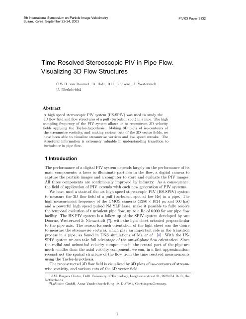
5th International Symposium on Particle Image VelocimetryBusan, Korea, September 22-24, 2003PIV’0 3 Paper 3132Time Resolved Stereoscopic PIV in Pipe Flow.Visualizing 3D Flow StructuresC.W.H. van Doorne1, B. Hof1, R.H. Lindken1, J. Westerweel1U. Dierksheide2AbstractAhigh speed stereoscopic PIV system (HS-SPIV) was used to study the3D flow field and flow structures of apuff (turbulent spot) in apipe. The highsampling frequency of the PIV system allows us to reconstruct 3D velocityfields applying the Taylor-hypothesis. Making 3D plots of iso-contours ofthe streamwise vorticity,and making various cuts of the 3D vector fields, wehave been able to visualize streamwise vortices and low speed streaks. Thestructural information is extremely valuable in understanding transition toturbulence in pipe flow.1 IntroductionThe performance of a digital PIV system depends largely on the performance of itsmain components: a laser to illuminate particles in the flow, a digital camera tocapture the particle images and a computer to store and evaluate the PIV images.All three components are continuously improved by industry. As a consequence,the field of application of PIV extends with each new generation of PIV systems.We have used a state-of-the-art high speed stereoscopic PIV (HS-SPIV) systemto measure the 3D flow field of a puff (turbulent spot at low Re) in a pipe. Thehigh measurement frequency of the CMOS cameras (1280 × 1024 px and 500 fps)and a powerful high speed pulsed Nd:YLF laser, make it possible to fully resolvethe temporal evolution of t urbulent pipe flow, up to a Re of 6 000 for our pipe flowfacility. The HS-PIV system is a follow up of the SPIV system developed by vanDoorne, Westerweel & Nieuwstadt [7], with the light sheet oriented perpendicularto the pipe axis. The reason for such orientation of the light sheet was the desireto measure the streamwise vortices, which play an important role in the transitionprocess in a pipe, as found in DNS simulations of Ma et al. [4]. With the HS-SPIV system we can take full advantage of the out-of-plane flow orientation. Sincethe radial and azimuthal velocity components in the central part of the pipe aremuch smaller than the axial velocity component, we can, in a first approximation,reconstruct the spatial structure of the flow from the time resolved measurementsusing the Taylor-hypothesis.The reconstructed 3D flow field is visualized by 3D plots of iso-contours of streamwisevorticity, and various cuts of the 3D vector field.1 J.M. Burgers Centre, Delft University of Technology, Leeghwaterstraat 21, 2628 CA Delft, theNetherlands2 LaVision GmbH, Anna-Vandenhoeck-Ring 19, D-37081, Goettingen,Germany.1

PIV’0 3 Paper 31322 Theoretical backgroundThe transition from laminar to turbulent pipe flow is still far from being understood.One of the difficulties is that the laminar parabolic velocity profile is linearlystable, which means that transition must start from a flow disturbance with finiteamplitude, although the disturbance may have any form. A sufficiently large andcontinuous perturbation will lead to a continuous turbulent flow in the pipe forRe 2 600, and for Re 1 800 all perturbations will eventually decay.For flow in the intermediate range of 1 800 Re 2 600, there will be coexistinglaminar and turbulent flow regions, even for very large initial perturbations.The turbulent regions are called ’puffs’ (Wygnanski & Champagne [12]). ForRe ≈ 2 200 the puff is in an equilibrium with its surrounding laminar flow (Wygnankiet al. [11]). The so-called equilibrium-puff does neither grow, nor shrink andtravels downstream trough the pipe at a velocity slightly below the bulk velocity(U puff ≈ 0.9U bulk ). At the upstream end of the puff there is a nett flow of laminarfluid entering the turbulent region, and therefore a continuous transition from laminarto turbulent flow occurs at this location. At the downstream end of the puff,the opposite process takes place. Turbulent fluid from the puff re-laminarises andleaves the puff.A puff represents a minimal flow unit for turbulent pipe flow, i.e. the smallestvolume in which a chaotic flow can be sustained given the Re. The flow dynamicsin a puff seems therefore a good starting point for understanding turbulence (ina pipe). Furthermore, it may be anticipated that the dynamics of the continuoustransition and the upstream side of a puff is also relevant for the transition at largerRe.3 Experimental setup and proceduresIn this section we describe the experimental setup and measurement procedure. Anoverview of the experimental parameters is presented in table 1, and a sketch ofthe SPIV system and the coordinate system is shown in figure 1. The High-Speed-Stereoscopic PIV (HS-SPIV) system used in this study is identical to the SPIVsystem described by van Doorne et al. [7], with exception of the cameras and thelaser.For our measurements we use a pipe flow facility with an inner diameter of 40mm and a total length of 28 m. A detailed description of the flow facility is givenby Draad [2]. The working fluid is water, and due to a well designed contractionand thermal isolation of the pipe, the flow can be kept laminar up to Re = 60 000.All measurements were carried out at 26 meters from the inlet.The PIV images were recorded with two High-Speed-Star-2 cameras from LaVision.The cameras have an 8-bit CMOS sensor with 1280×1024 px (pixel). The maximumimage frame rate is 500 Hz, and can be reduced to 250, 125 and 60 Hz. Theadjustment of the timing of the laser pulses and camera shutters makes it possibleto change the PIV delay time between two subsequent images, just as for contemporarycross-correlation cameras, with a minimum delay time of 8 µs. It is possibleto record 1 000 frames, which corresponds to a recording time of 2 seconds at themaximum frame rate. The frequency of the cameras can be further increased at thecost of a reduced image format (e.g., 16 kHz for 32×320 px). Both cameras lookat an angle of 45 degrees to the object plane and satisfy the Scheimpflug condition.The cameras are placed in the forward scattering direction of the laser light andtherefore stand on different sides of the light sheet (Willert [10]).Sphericel particles with a nominal diameter of 10 µm were added to the waterto increase the particle density. A substantial part of the particles remains in2

PIV’0 3 Paper 3132Nd:YLF−laser lenses mirror on traversetraversing directiontest sectionxy z= 40 mm45water prismsCMOS cameras onScheimpflug mountFigure 1: Schematic of High Speed Stereoscopic-PIV system. The coordinate systemis also indicated in the graph.Table 1: Overview of relevant parameters of the experimental setup.Pipe diameter 40 mmlength 30 mwall thickness 1.6 mmFlow fluid waterReynolds number 2000bulk velocity 50 mm/sSeeding type Sphericlediameter 10 µmLight sheet laser type Nd:YLFmaximum energy 10 mJ/pulsthickness 1.5 mmRecording camera type CMOSviewing angle 45 degreesresolution 1280×1024 pxframe rate 125 Hzlens focal length 105 mmf-number 2.8image magnification 0.35viewing area 40×45 mm 2exposure delay time 4 msmaximum particle displacement 8 pxInterrogation method 3D calibrationinterrogation area 32×32 pxinterrogation area 1.4×1.4 mm 2laser sheet3

PIV’0 3 Paper 3132suspension, and makes it possible to measure in both laminar and transitional flows.The flow is illuminated by a pulsed dual-cavity DPPS Nd:YLF laser with a maximumenergy of 10 mJ per pulse per laser head at a repetition rate of 1000 Hz (NewWave Pegasus-PIV-30W). The laser beam diameter is approximately 1.5 mm andthe wavelength of the light is 527 nm. The light sheet is formed with two lenses,and a mirror on a micro traverse makes it possible to adjust the position of the lightsheet.To minimize optical distortion of the image, the pipe inside the test section isreplaced by a 1.6 mm thick glass tube and two water prisms are placed in front ofthe test section (Prasad 2000).The light sheet is perpendicular to the mean flow direction in order to capturethe flow over the entire cross-section of the pipe and to be able to reconstruct the3D velocity field from the recorded time sequence. The light sheet thickness has adirect influence on the accuracy of the velocity measurements (van Doorne et al.[7]). We used a light sheet thickness of approximately 1.5 mm, which is a goodcompromise between the spatial resolution and the signal-to-noise ratio. Particledisplacements of up to 8 pixels (0.45 mm) result in a strong correlation, and we canresolve displacements with a precision of 0.1 pixel.The reconstruction of the 3C-vector fields from the two displacement fields ofthe cameras is based on a 3D calibration of the SPIV system (Soloff et al. [6],Prasad [5]). The calibration grid is recorded at two z-positions (instead of one fora 2D calibration), and the method does not require the input of any geometricparameter of the setup.The data acquisition system is a commercial system from LaVision including thesoftware (Davis 6.3.1) for the evaluation of the vector fields. The vector analysis isdone in two steps. In the first step we use 32×32-pixel fixed interrogation windows,after which spurious vectors were detected with a median filter (Westerweel [8]) andreplaced by either a vector of a lower correlation peak or an interpolation of theneighboring vectors. In the second step we also used 32×32-pixel interrogation regions,and the vector fields of the first step are used for pre-shifting (Westerweel et al.[9]). Again spurious vectors are removed and, if possible, replaced by a vector froma lower correlation peak; spurious vectors are not replaced by interpolated data.After this the vector fields of both cameras are dewarped and recombined (usingthe 3D calibration) to obtain the 3C-vector field.For a discussion of details such as the applied calibration grid, the calibration procedureand the procedure to align the laser sheet with the calibration plane, to eliminatethe effects of the registration error, we refer to the paper by van Doorne et al.[7]. They performed a detailed analysis of the accuracy of the SPIV system with alarge out of plane motion. It was found that the SPIV system was able to measurethe velocity with high accuracy over the entire cross-section of the pipe. The noiselevel of individual vectors was smaller than 0.1 px and the turbulence statistics werein excellent agreement with those of the DNS computations by Eggels et al. [3].These experiments were repeated with the HS-SPIV system, and identical resultswere found.4 ResultsAll the results that will be presented in this section are based on a single measurementof a puff at Re = 2 000. The results will illustrate some of the new possibilitiesoffered by the high speed PIV measurements.The camera frame rate used for this experiment was 125 Hz, which gave us ameasurement time of 8 s. Because the PIV-delay-time was set to 4 ms, the actualmeasurement frequency was 62.5 Hz. We did not use the maximum camera speed4

PIV’0 3 Paper 313250mean axial velocity (mm/s)4030201047.647.447.2magnified view470 4 800 2 4 6 8time (s)Figure 2: Mean axial velocity averaged over the pipe cross-section as a function oftime.(500 Hz) because the corresponding measurement time of 2 s was too short tocapture the entire passage of the puff, which takes about 10 s.Two results that confirm the accuracy of the measurement equipment are thegraphs of the bulk velocity (figure 2) and the probability density functions (PDF)of the three velocity components (figures 3 and 4). The bulk velocity is calculatedas the average axial velocity over the cross-section of the pipe. The mean bulkvelocity is 47.3 mm/s and the root mean square (rms) of the bulk velocity is 0.085mm/s, which is 0.18% of the mean bulk velocity. From the trend in the graph wecan see that there was a small change in the flow rate due to pump fluctuations andtherefore the measurement uncertainty in the flow rate is estimated to be slightlysmaller than 0.18%.The PDFs in figure 3 show a small asymmetry in the measurement of the u xand the u y velocity components (from now on referred to as the in-plane velocitycomponents). From the symmetry of the pipe flow one would expect that the twoPDFs are identical. A possible explanation is that the PIV-interrogation noise in u yis about 0.7 (∼ 2√ 1 2) smaller than the noise in ux , because it is the average of twoindependent measurements of camera 1 and camera 2 (Prasad [5], van Doorne et al.[7]). The PDF of u z in figure 4 shows a small degree of peak-locking to integerpixel values. Furthermore it can be seen that the occurrence of small velocities issomewhat overestimated, which is due to an underestimation of the axial velocityand an increased noise level in the near wall region, caused by bright tracer particlesattached to the wall.The time trace of the axial velocity at the centerline of the pipe is shown infigure 5. We have captured the active region of the puff, around the trailing edgewhich is located at about 6 s. This is only a part of the full signature of a puff as it isknown in literature (Wygnanski & Champagne [12], Darbyshire & Mullin [1]). Thegradual decrease of the centerline velocity (the leading edge) that is often shownprecedes the beginning of our measurement. The leading edge is the region wherethe flow re-laminarises, and the laminar profile is restored by the growth of the5

PIV’0 3 Paper 3132in−plane velocity (mm/s)−15 −10 −5 0 5 10 155u x4u yprobability (1/px)3210−1.5 −1 −0.5 0 0.5 1 1.5particle displacement (px)Figure 3: Probability density function of the in-plane velocity components as measuredover the entire passage of the puff.0.25axial velocity (mm/s)0 20 40 60 80u z0.2probability (1/px)0.150.10.0500 1 2 3 4 5 6 7 8particle displacement (px)Figure 4: Probability density function of the axial velocity.6

PIV’0 3 Paper 3132u z(r=0) (mm/s)959085807570658.587.576.56particle displacement (px)600 1 2 3 4 5 6 7 8time (s)Figure 5: Axial velocity on the center line of the pipe.boundary layers from the wall. From a dynamical point of view this region is oflittle interest. An indication of the noise level is given by the right end of the graph,for t > 6 s. The flow is laminar in this region (upstream from the puff) and therapid fluctuations are due to the PIV interrogation noise of the order of 0.1 px.Figure 6 shows the kinetic energy of the in-plane velocity and it can be seen thatthe flow has indeed relaminarised upstream of the beginning of our measurement.The kinetic energy of the in-plane velocity is calculated as the mean value of 〈u 2 x+u 2 y〉over the cross-section of the pipe. Several interesting points can be observed. Firstof all, there is a very large and sharp peak in the kinetic energy of the in-planevelocity. At conventional sampling rates of 7 or 15 Hz, this peak would not havebeen properly resolved and might have been rejected as noise. Figure 8(c) showsthe in-plane velocity field that corresponds to the peak in the kinetic energy. Avery strong cross-flow extends over almost the entire cross-section of the pipe, and aremarkable feature is the highly symmetric configuration of the streamwise vorticity.Further investigation might reveal the relevance and/or dynamics of such vigorousand isolated mixing of the flow.Another interesting point is the rapid increase of the total kinetic energy fort > 6 s (figure 7). In order to understand the transition it may be useful to studythe flow in an Lagrangian frame of reference that moves with the fluid. Laminar fluidinitially upstream of the puff continuously enters the puff and undergoes transitionto turbulence. Traveling with the fluid, we should thus read the figure from right toleft. We then see that subststantial fracion of the kinetic energy of the streamwisevelocity will be lost (due to changes in the mean profile), even before the flow hasbecome fully turbulent and the turbulence could have increased the dissipation ofthe kinetic energy. We find this quite surprising, and this might indicate that thepressure plays an important role in the energy redistribution in this region. Thesespeculations of course will be subject of further investigations.A 3D visualization of the iso-surfaces of the streamwise vorticity in the puff isshown in figure 9. Since the velocity fluctuations are much smaller than the meandownstream velocity, we can, in a first approximation, apply the Taylor hypothesisto convert time into space. The z-coordinate has actually been calculated by multi-7

PIV’0 3 Paper 3132x 10 −5< u x2 +uy2 > (mm/s)24200 1 2 3 4 5 6 7 8time (s)Figure 6: Kinetic energy of the in-plane velocity.4 x 10−4 2 −3 − 2.6×10 z2 2xtime (s)mean kinetic energy (mm/s) 232100 1 2 3 4 5 6 7 8Figure 7: Kinetic Energy of the in-plane and axial velocity8

PIV’0 3 Paper 313220 time = 2 s 10 mm/s20 time = 3 s 10 mm/s101000−10−10(a)(b)−20−20−20 −10 0 10 20 −20 −10 0 10 2020 time = 5.4 s 10 mm/s20 time = 6.3 s 10 mm/s101000−10−10(d)−20−20 −10 0 10 20(e)−20−20 −10 0 10 20Figure 8: Inplane velocity fields and axial vorticity at different instance of time.Sub-figure c is at the moment of maximal in-plane kinetic energy, see figure 6.9

PIV’0 3 Paper 3132Figure 9: 3D visualization of the iso-contours of streamwise vorticity (± 5.5 s −1 ) inthe puff. The letters on the z-axis refere to the sub-figures of figure 8.plication of the measurement time and bulk velocity. The flow structures visualizedin the reconstructed 3D flow field may not have the exact shape and orientation asin the real flow, but we expect the qualitative picture to be correct.From figures 8 and 9, and from movies that were not presented in this paper,it appears that the transition at the upstream end of the puff starts with the appearanceof weak low speed streaks and streamwise vortices close to the wall. Thestreaks and vortices grow and eventually breakdown to result in a turbulent flow.The appearance of the first streaks and streamwise vortices is rather chaoticallydistributed along the circumference of the pipe. So far we have not been able tofind any clear organization in the late stages of the transition and the interior ofthe puff. Even at these very low Re the flow dynamics of the transition is verycomplicated and chaotic.5 Conclusion and discussionA state of the art high speed stereoscopic PIV (HS-SPIV) system was used for thestudy of laminar turbulent transition in a puff in pipe flow. The HS-SPIV systemhas the same accuracy as a conventional SPIV system. The high sampling rate hasmade it possible to fully resolve the temporal evolution of the flow (at 500 Hz upto Re = 6 000 for our setup) and access complicated quantities such as the timeevolution of the kinetic energy.The 3D flow field of a puff was reconstructed from the time resolved measurementsby application of the Taylor-hypothesis to convert time to space. In particular thismeasurement revealed a large spike in the kinetic energy. At conventional samplingrates of 7 or 15 Hz, this spike would probably not have been discovered. Thestreamwise vortices were visualized by means of a 3D plot of the iso-contours of the10

PIV’0 3 Paper 3132vorticity.We conclude that the high speed SPIV technique applied to a cross-flow canmeasure 3D flow fields and reveal its 3D flow structure, which so far was onlypossible with (DNS) calculations.In the near future we will further explore the data set of several other puffs thatwere recorded at different Re. Measurements at 500 Hz were also performed forfully developed turbulent flow at Re = 3 000 and Re = 5 300 and for turbulent flowwith drag reducing polymers. We also plan to extract the 3D vorticity vector fieldfrom the 3D velocity fields.References[1] A.G. Darbyshire and T. Mullin. Transition to turbulence in constant-mass-fluxpipe flow. J. Fluid Mech., 289:83–114, 1995.[2] A.A. Draad. Laminar-turbulent transition in pipe flow for Newtonian and non-Newtonian fluids. PhD thesis, Delft Universtity of Technology, 1998.[3] J.G.M. Eggels, J. Westerweel, and F.T.M. Nieuwstadt. Direct numerical simulationof turbulent pipe flow. Appl. Sci. Res., 51:319–324, 1993.[4] B. Ma, C.W.H. Doorne, Z. Zhang, and F.T.M. Nieuwstadt. On the spatialevolution of a wall-imposed periodic disturbance in pipe poiseuille flow at re =3000. part1. sub-critical disturbance,. J. Fluid Mech., 398:181–224, 1999.[5] A.K. Prasad. Stereoscopic particle image velocimetry. Exp. Fluids, 29:103–116,2000.[6] S.M. Soloff, R.J. Adrian, and Z.C. Liu. Distortion compensation for generalisedstereoscopic particle image velocimetry. Meas. Sci. Technol., 8:1441–1454, 1997.[7] C.W.H. van Doorne, J. Westerweel, and F.T.M. Nieuwstadt. Measurementuncertainty of stereoscopic-piv for flow with large out-of-plane motion. In Proceedingsof the EUROPIV 2 final workshop on Particle Image Velocimetry,Zaragoza, Spain. Springer Verlag, 2003.[8] J. Westerweel. Efficient detection of spurious vectors in particle image velocimetrydata. Exp. Fluids, 16:236–247, 1994.[9] J. Westerweel, D. Dabiri, and M. Gharib. The effect to a discrete windowoffset on the accuracy of cross-correlation analysis of digital piv recordings.Exp. Fluids, 23:20–28, 1997.[10] C. Willert. Stereoscopic digital particle image velocimetry for application inwind tunnel flows. Meas. Sci. Technol., 8:1465–1479, 1997.[11] I. Wygnanski, M. Sokolov, and D. Friedman. On transition in a pipe. part 2.the equilibrium puff. J. Fluid Mech., 69:283–304, 1975.[12] I.J. Wygnanski and F.H. Champagne. On transition in a pipe. part 1. the originof puffs and slugs and the flow in a turbulent slug. J. Fluid Mech., 59:281–335,1973.11