Detecting natural influence on surface air temperature ... - IMAGe

More documents

Recommendations

Info

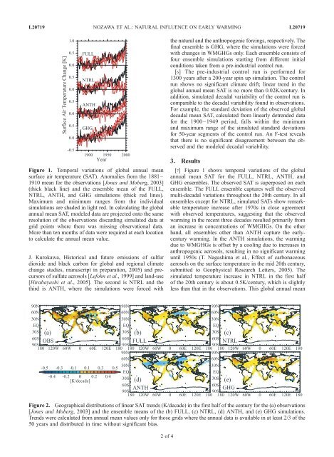
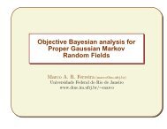
L20719 NOZAWA ET AL.: NATURAL INFLUENCE ON EARLY WARMING L20719the <strong>natural</strong> and the anthropogenic forcings, respectively. Thefinal ensemble is GHG, where the simulations were forcedwith changes in WMGHGs only. Each ensemble consists offour ensemble simulations starting from different initialconditions taken from a pre-industrial control run.[6] The pre-industrial control run is performed for1300 years after a 200-year spin up simulation. The controlrun shows no significant climate drift; linear trend in theglobal annual mean SAT is no more than 0.02K/century. Inaddition, simulated decadal variability of the control run iscomparable to the decadal variability found in observations.For example, the standard deviation of the observed globaldecadal mean SAT, calculated from linearly detrended datafor the 1900–1949 period, falls within the minimumand maximum range of the simulated standard deviationsfor 50-year segments of the control run. An F-test revealsthat there is no significant disagreement between the observedand the modeled decadal variability.Figure 1. Temporal variations of global annual meansurface air temperature (SAT). Anomalies from the 1881–1910 mean for the observations [Jones and Moberg, 2003](thick black line) and the ensemble mean of the FULL,NTRL, ANTH, and GHG simulations (thick red lines).Maximum and minimum ranges from the individualsimulations are shaded in light red. In calculating the globalannual mean SAT, modeled data are projected onto the sameresolution of the observations discarding simulated data atgrid points where there was missing observational data.More than ten months of data were required at each locationto calculate the annual mean value.J. Kurokawa, Historical and future emissions of sulfurdioxide and black carbon for global and regional climatechange studies, manuscript in preparation, 2005) and precursorsof sulfate aerosols [Lefohn et al., 1999] and land-use[Hirabayashi et al., 2005]. The second is NTRL and thethird is ANTH, where the simulations were forced with3. Results[7] Figure 1 shows temporal variations of the globalannual mean SAT for the FULL, NTRL, ANTH, andGHG ensembles. The observed SAT is superposed on eachensemble. The FULL ensemble captures well the observedmulti-decadal variations throughout the 20th century. In allensembles except for NTRL, simulated SATs show remarkabletemperature increase after 1970s in close agreementwith observed temperatures, suggesting that the observedwarming in the recent three decades resulted primarily froman increase in concentrations of WMGHGs. On the otherhand, all ensembles other than ANTH capture the earlycenturywarming. In the ANTH simulations, the warmingdue to WMGHGs is offset by a cooling due to increases inanthropogenic aerosols, resulting in no significant warminguntil 1950s (T. Nagashima et al., Effect of carbonaceousaerosols on the surface temperature in the mid 20th century,submitted to Geophysical Research Letters, 2005). Thesimulated temperature increase in NTRL in the first halfof the 20th century is about 0.5K/century, which is slightlyless than that in the observations. This global annual meanFigure 2. Geographical distributions of linear SAT trends (K/decade) in the first half of the century for the (a) observations[Jones and Moberg, 2003] and the ensemble means of the (b) FULL, (c) NTRL, (d) ANTH, and (e) GHG simulations.Trends were calculated from annual mean values only for those grids where the annual data is available in at least 2/3 of the50 years and distributed in time without significant bias.2of4
L20719 NOZAWA ET AL.: NATURAL INFLUENCE ON EARLY WARMING L20719Figure 3. Best-estimated (a, b) signal amplitudes and (c, d)linear trends (K/century) with 5–95% uncertainty ranges forthe 50-year segment from 1900 to 1949 for the GHG,ANTH-GHG (anthropogenic signal other than WMGHGs)(Figures 3a and 3c), and the NTRL analysis and for theANTH and NTRL analysis (Figures 3b and 3d). The orangeerror bar with an asterisk, green error bar with a diamond,light green error bar with a cross, and blue error bar with atriangle indicates GHG, ANTH-GHG, ANTH, and NTRL,respectively. Also shown in Figures 3c and 3d are the totalreconstructed trend from the regression model (red error barwith a plus) and the observed (solid error bar with a square)trend. Error bars denote 5–95% uncertainty ranges.SAT trend in NTRL is larger than that of Stott et al. [2000]and T02 (0.3K/century) for their simulations with <strong>natural</strong>forcings only, although we use identical <strong>natural</strong> forcingdatasets to the ones they used. The trend of the globalannual mean SAT in GHG is nearly equal to that in NTRL;therefore, without further investigation, we cannot concludewhich factors are the main contributors to the observedearly warming.[8] Geographical distributions of linear SAT trends forthe first half of the century are shown in Figure 2 for theobservations and the ensemble mean of each ensemble. Thetrend patterns in NTRL as well as in FULL (Figures 2band 2c) compare quite favorably with the trend patterndrawn from the observations (Figure 2a). In the ANTHsimulations, on the other hand, the indirect effect ofanthropogenic aerosols introduces cooling trends in theNorth America and the Northern Atlantic (Figure 2d),where the observed warming was largest in this period(1900–1949) (Figure 2a). The trend pattern in GHG(Figure 2e) looks less similar to the trends in the observationsthan do the trends in NTRL.[9] To clarify the relative importance of the effect ofWMGHGs and <strong>natural</strong> <strong>influence</strong>s on the warming in theearly 20th century, an optimal detection method usingtotal least squares regression (TLS) [Allen and Stott,2003] was applied to the simulated and observed SAT.In contrast to ordinary least squares regression (OLS), aswas used in many previous studies (e.g., T02), TLS takesinto account sampling uncertainty in the model responseswhen estimating the signal amplitudes, and gives anunbiased regression coefficient. Similar to the analysisof T02, we regress the observed spatio-temporal variationsonto the three model-derived response patterns fromGHG, ANTH, and NTRL to estimate the signal amplitudesfor GHG, ANTH-GHG (i.e., the temperature responseto all the anthropogenic <strong>influence</strong>s exceptWMGHGs) and NTRL effects. The signal amplitude forANTH-GHG is computed via a linear transformation fromthe GHG and ANTH responses (see T02 for moredetails). Following the approach of Stott et al. [2001]the observed and simulated SATs in the early 20thcentury (1900–1949) were averaged decadally, expressedas anomalies with respect to the same period, and filteredby projecting onto T4 spherical harmonics. We calculatethe signal amplitudes by estimating covariance matrices,for optimization, from intra-ensemble spread of theensembles using a truncation of 10 EOFs. Applying theresidual test of Allen and Tett [1999], we found thatthe residual in the regression was consistent with controlvariability. The uncertainty on the amplitudes was estimatedfrom our 1300-year control simulation.[10] The estimated signal amplitudes and uncertaintyranges (Figure 3a) indicate that, unlike with T02, only the<strong>natural</strong> contribution is detectable (i.e., only the uncertaintyrange for NTRL is entirely positive), and since the uncertaintyrange includes unity, the signal amplitude is consistentwith the amplitude of the signal in observations. Itshould also be noted that the detection of the NTRL signaland its consistency with the observations is independent ofthe number of EOFs retained in the analysis (not shown).Therefore the detected <strong>natural</strong> contribution is robust. Thetwo anthropogenic signals, on the other hand, have largeuncertainty and are not detectable. Again this result isindependent of number of EOFs retained in the analysis(not shown). To make a direct comparison with the analysisof T02, we repeated our analysis using OLS. We found thatthe best-estimated signal amplitudes are not largely differentfrom those shown in Figure 3a (calculated with TLS).However, since OLS assume no sampling uncertainty inthe model responses, the estimated uncertainty limits aresmaller with OLS than those with TLS (not shown). Itshould be noted that, unlike with T02, the two anthropogenicsignals have large uncertainty and are not detectedeven in our OLS analysis.[11] Figure 3c shows best-estimated linear trend for theearly half of the century. The total trend shows much betteragreement with the observations than that in T02. Note thatthe best-estimated trends in Figure 3c are also not largelydifferent from those with OLS. The <strong>natural</strong> forcing causes awarming trend of 0.6K/century, which is about one half ofthe observed trend. This is consistent with the global annualmean SAT anomalies simulated in NTRL (Figure 1). Theresidual of the observed trend (0.4K/century) may becaused by the combined anthropogenic forcings, primarilyby the WMGHGs. However, the two anthropogenic signalsare highly uncertain and are not detected. Therefore thecause of the residual trend is not obvious.[12] The robustness of the NTRL signal is tested byregressing the observations onto the two simulatedresponses from ANTH and NTRL (Figures 3b and 3d).Again, only the <strong>natural</strong> contribution is detected while thenet anthropogenic signal is highly uncertain and is notdetected. This confirms the significance of the <strong>natural</strong>contributions to the early 20th century warming.4. Concluding Remarks[13] Surface air temperature changes simulated by aglobal coupled climate model with different external forcingsare investigated to detect the observed climate changesignals in the early 20th century. Unlike with several3of4
Page 1: GEOPHYSICAL RESEARCH LETTERS, VOL.

Detecting natural influence on surface air temperature ... - IMAGe

Create successful ePaper yourself

Delete template?

Save as template?