A Spatial Analysis of Multivariate Output from Regional ... - IMAGe

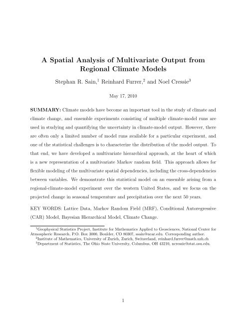
tistical model to capture the multivariate spatial distribution of the output fields (e.g., thejoint spatial distribution of temperature and precipitation) from a regional-climate-modelensemble. With this statistical representation of the model output, we can present probabilisticprojections of regional climate change based on the ensemble. Furthermore, byconsidering multiple output fields simultaneously, we can incorporate correlations betweenthese fields, improving joint projections necessary for many climate-impacts studies (e.g.,agriculture, water management, public health, etc.)1.1 Regional Climate ModelsThe climate of a region is determined by processes that exist at planetary, regional, and localspatial scales and across a wide range of temporal scales (multi-decadal to sub-daily). Thiscreates serious difficulties when attempting to construct computer models that can simulateregional climate. Atmosphere-ocean general circulation models (AOGCMs or, more simply,GCMs) couple an atmospheric model with an ocean model and seek to simulate the Earth’sglobal climate system. Due to model complexity, the need to simulate climate over decadaland even centennial time scales, and computational limitations, these models typically havegrid boxes on the spatial scale of 200 to 500 km. While these models are extremely useful forinvestigating the large-scale circulation and forcings that affect the Earth’s global climate,there are limitations to their use for regional and local projections that might be of interestto the climate-impacts community.Recognizing the need to include large-scale processes, even when studying regional climate,as well as the ability of GCMs to capture such phenomena, there is considerableattention on developing downscaling methodologies. Downscaling refers simply to generatinginformation on the basis of a GCM, but at spatial scales below that of the GCM. Thereare two main types of downscaling, dynamical and statistical. Statistical downscaling is acomputationally efficient approach that uses empirical relationships to connect the coarseresolutionGCM output to regional and local variables. This approach needs fine-scale andlong-time-duration observational data, and there is some uncertainty about the stability3

of these empirical relationships over long periods of time, especially with varying forcings(e.g., increasing CO 2 concentrations).Dynamical downscaling involves using high-resolution climate models. Of course, thereare limitations due to computational demands and a price to be paid for the higher resolution.One approach uses only the atmospheric component of a GCM with, for example,observed ocean temperatures. These so-called time-slice experiments are globally consistent,but they generally use many of the same formulations as the coarse-scale GCMs.Regional climate models (RCMs) are the focus of this research and are another dynamicalapproach based on high-resolution climate models. These models typical focus on alimited spatial domain, have grid boxes on the scale of 20 to 100 km, and there are oftensimplifications of ocean processes in these models. They also use initial conditions andtime-dependent lateral boundary conditions from the GCM (e.g., winds, temperature, andmoisture). Hence, global circulation and large-scale forcings are consistent with the GCM,but, with the higher-resolution forcings included (e.g., topography, land cover, etc.), thesemodels have the potential to actually enhance the simulation of climate on regional andlocal scales. Of course, RCMs can be influenced by potential biases in the GCM, and thereis a lack of two-way interactions between the driving GCM and the RCM.For those interested in understanding more about climate and climate change and globaland regional climate modeling, we refer them to the Intergovernmental Panel on ClimateChange (IPCC, http://www.ipcc.ch) assessment reports, and in particular to the contributionsof Working Group I to the Third Assessment Report (Houghton et al., 2001) andthe Fourth Assessment Report (Solomon et al., 2007). These documents not only includeexcellent overviews of the issues but also numerous scientific references for more in-depthcoverage.1.2 A Statistical Representation of Climate-Model OutputWe propose a statistical model for combining the output from simple ensembles of RCMsin order to characterize the distribution of the model output. This statistical model will be4

dependence through the specification of a covariance function (typically based on distancesbetween spatial locations), Gaussian MRF models represent the conditional expectation ofan observation at a spatial location as a linear combination of observations at neighboringlocations. Spatial dependence is induced through this conditional autoregression and thechoice of neighborhoods.In addition, using a MRF formulation will allow us to incorporate computational advantagesdue to the gridded nature of the climate-model output and the sparseness that ischaracteristic of the spatial-precision matrices (inverse covariance matrices) that are specifiedin such models. Furthermore, the multivariate nature of the statistical model (morethan one model output considered at each grid box) will allow for more complex inferencesthat are of use to those studying impacts of climate and climate change.1.3 OutlineIn Section 2, an overview of MRF models is presented, followed by a description of the newformulation in Section 3. Section 4 contains the details of our hierarchical specification.An extensive study of an application using a simple ensemble of RCM output, focusing onchanges in seasonal temperature and precipitation, will be presented in Section 5. Concludingremarks are given in Section 6.2 MRF and CAR ModelsBesag (1974) laid out the basic framework for MRF models. For random variables y 1 , . . . , y nobserved at n locations on a spatial-lattice structure, the collection of conditional distributionsf(y i |y −i ), i = 1, . . . , n (where y −i refers to all random variables except the ithone), can be combined under certain regularity conditions to form a joint distributionf(y 1 , . . . , y n ). Rue and Held (2005) can be consulted for an excellent exposition of the theoryof MRFs; see also the reviews in the texts by Cressie (1993), Banerjee et al. (2004), andSchabenberger and Gotway (2005). Conditional autoregressive (CAR) models are specialcases of MRF models where the conditional distributions are assumed to be Gaussian.6

2.1 Univariate CAR ModelsIn the univariate setting and assuming Gaussian conditional distributions for f(y i |y −i ), theconditional mean and conditional variance associated with f(y i |y −i ) are specified asE[y i |y −i ] = µ i +n∑b ij (y j − µ j ) and Var[y i |y −i ] = τi 2 > 0,j≠iwhere b ii = 0; i = 1, . . . , n. Under regularity conditions, this collection of conditionaldistributions gives rise to a joint Gaussian distribution,N ( µ, (I − B) −1 T ) , (1)where µ = (µ 1 , . . . , µ n ) ′ , I is an n × n identity matrix, B is the n × n matrix with the(i, j)-th element b ij , and T = diag(τ1 2 , . . . , τn). 2 The regularity conditions are on the spatialdependenceparameters, {b ij }, and they ensure that the resulting matrix, (I − B) −1 T, is abona fide covariance matrix; that is, (I − B) −1 T is symmetric and positive-definite. Thespatial dependence is induced by the autoregression, which is determined by setting thecoefficients b ij ≠ 0 if j ∈ N i (and 0 otherwise), where N i is a collection of indices thatdefine a neighborhood of the ith location in the spatial lattice.2.2 Multivariate CAR ModelsMardia (1988) extended the MRF model of Besag (1974) to the multivariate setting wherethere is more than one measurement at each lattice point. In particular, let y i be a p-dimensional random vector. Then, for i = 1, . . . , n, let f(y i |y −i ) be a Gaussian distributionof y i , given all random vectors except the ith, withE[y i |y −i ] = µ i + ∑ B ij (y j − µ j ) and Var[y i |y −i ] = T i ,j≠iwhere µ i is a p-dimensional vector, B ij is a p × p matrix, and T i is a p × p covariancematrix. Assume that B ij T j = T i B ′ ji, for all i, j = 1, . . . , n (to ensure symmetry). Further,assume B ii = −I and B ij ≠ 0 for j ∈ N i and i = 1, . . . , n. Under the assumption that the7

np × np matrix Block(−B ij ) (i.e., a block matrix with blocks given by −B ij ) is positivedefinite,Mardia (1988) establishes that y = (y ′ 1, . . . , y ′ n) ′ follows a N (µ, Σ) distributionwhere µ = (µ ′ 1, . . . , µ ′ n) ′ and Σ = ( Block(−T −1i B ij ) ) −1.As written, this formulation is overparameterized and there have been a number ofefforts in the literature that focus on ways of specifying the parameters in the basic model.See, for example, Billheimer et al. (1997), Kim et al. (2001), Pettitt et al. (2002), Carlinand Banerjee (2003), Gelfand and Vounatsou (2003), Jin et al. (2005, 2007), Daniels et al.(2006), Sain and Cressie (2007), among others.3 An Alternative Formulation of a Multivariate MRFIt is our experience that the basic multivariate MRF model of Mardia (1988) is difficultto implement in practice without dramatic simplification of the matrices representing thespatial dependence parameters (e.g., Billheimer et al., 1997) or the use of restrictive priorson the elements of these same matrices (Sain and Cressie, 2007). Here, we fully develop anew way of representing multivariate lattice data that was suggested, but not implemented,by Sain and Cressie (2007), for the purposes of analyzing an RCM experiment.The multivariate extension of the framework laid out by Besag (1974) and explored byMardia (1988) is based on the assumption of a multivariate observation at each point ona standard two-dimensional spatial lattice. Fundamental to our approach is thinking ofmultivariate lattice data as univariate data on a more complex lattice structure.In particular, this more complex lattice structure is conceptualized as a “stacking”of the lattices associated with each variable. Neighborhoods are defined by connectionsbetween locations for each variable within a lattice and again for locations across each latticestructure. A two-dimensional example of these different types of neighborhoods is shownin Figure 1. A within-variable dependence structure is induced by connecting locationswithin a lattice associated with a particular variable (left frame). Cross-dependencies, bothwithin a location (middle frame) and across locations (right frame), are induced throughconnections between the lattices for different variables.8

Figure 1: Examples of different types of neighborhoods. The left frame shows a withinvariablespatial neighborhood, while the middle frame shows a within-location neighborhood.The right frame demonstrates the neighborhood associated with cross-variable connections.See also Eqn. (2).The key feature of this approach is that it still falls within the original univariateframework of Besag (1974) outlined in Section 2.1. Let y ij denote the jth variable observedat the ith location on the lattice. Then, for each Gaussian conditional distribution, themean and variance need to be specified. With sums on the right-hand side correspondingto specific types of neighborhoods in Figure 1, the conditional mean is given byE[y ij |y −{ij} ] = µ ij + ∑ b ijkj (y kj − µ kj ) + ∑ b ijil (y il − µ il ) + ∑b ijkl (y kl − µ kl ) (2)k≠il≠jk,l≠i,jwith the conditional variance given by Var[y ij |y −{ij} ] = τij, 2 for all lattice points i = 1, . . . , n,variables j = 1, . . . , p, and with y −{ij} denoting all components of y except for the (i, j)-th.In the conditional mean, the coefficients in the first summation, {b ijkj ; i = 1, . . . , n, k ∈N i , j = 1, . . . , p}, represent connections within a particular layer and control conditionaldependence between the ith lattice point and neighboring points for the jth variable (leftframe in Figure 1). The coefficients in the second summation, {b ijil ; i = 1, . . . , n, j ≠l = 1, . . . , p}, represent connections across layers at the same lattice point and controlconditional dependence between variables j and l at the ith lattice point (middle framein Figure 1). Finally, the coefficients in the third summation, {b ijkl ; i = 1, . . . , n, k ∈N i , j ≠ l = 1, . . . , p}, represent connections between locations across layers for different9

The specifications above simply ensure symmetry and reduce the number of parametersthat must be estimated. Of course, the collection of spatial-dependence parameters, {ρ jl }and {φ jl }, must be chosen to ensure that (5) is a positive-definite covariance matrix. Thefinal model has p(p − 1)/2 within-location dependence parameters, {ρ jl }, and p 2 betweenlocationspatial-dependence parameters, {φ jl }, in addition to the p variance parameters,{τj 2 }, and any parameters that are used to define the means.4 A Hierarchical Model for an RCM ExperimentLet the n-dimensional vector y rj denote the output of an RCM, in particular the rthensemble member for the jth variable. In this work, we focus solely on simple ensembles;that is, each member of the ensemble represents a perturbation of initial conditions for asingle model. Potential extensions of this basic framework for perturbed physics or multimodelensembles is discussed in Section 6.At the first level of the hierarchy, the data model assumes that the vectors y rj , r =1, . . . , m, j = 1, . . . , p, are independent withy rj |α j , β rj , h rj , σj 2 ∼ N ( X 1 α j + X 2 β rj + h rj , σ j I ) , (6)where m indicates the number of ensemble members. In the mean structure, we allow forfixed effects common to all ensemble members within the jth variable (X 1 α j ) and randomeffects specific to the rth ensemble member within the jth variable (X 2 β rj ). Spatial randomeffects are included through h rj , and σ j represents a variable-specific variance.The process model has two parts. First, the vectors [β ′ r1, . . . , β ′ rp] ′ , r = 1, . . . , m, areassumed to be independent with⎛ ⎞⎛β r1⎜ ⎟⎜⎝ . ⎠⎝β rp∣⎞⎛⎛β 1⎟⎜⎜. ⎠ , Σ b ∼ N ⎝⎝β p⎞ ⎞β 1⎟ ⎟. ⎠ , Σ b ⎠ , (7)β pwhere Σ b is a pq × pq covariance matrix with q the number of columns of X 2 . Second, the12

Figure 2: Top row shows the three differences in winter midpoint temperature ( o K), whilethe bottom row shows the three differences in total precipitation (inches).January, and February) average temperature and average total precipitation, were computedfor each grid box and for each of the control and the three future runs. Differencesbetween the future and the control were calculated, yielding change-in-temperature andchange-in-total-precipitation variables. Hence, there are p = 2 variables and m = 3 ensemblemembers, giving six fields to be analyzed. These spatial fields for the winter season areshown in Figure 2. A second, separate analysis with the same structure is also presentedfor the twenty-year summer (June, July, and August) change in temperature and changein total precipitation.We note that the statistical models outlined in this work focus on using Gaussianassumptions for average precipitation from an RCM. (An assumption that was verifiedthrough exploratory analysis.) However, other models for precipitation, in particular forextreme precipitation, are possible; see, for example, Sansó and Guenni (2004), Schliepet al. (2010), and Cooley and Sain (2010).15

5.1 Model SpecificationWe now outline some specifics about the statistical-model specification. Consider the datamodel (6).After some exploratory analysis, (scaled) latitude, longitude, and elevationwere used as covariates in the common regression component (X 1 α j ), to which a randomintercept across ensemble members was added (X 2 β rj ). The prior covariance matrix forthe random intercept in (7) was also simplified to Σ b = σ 2 b I p.The prior distribution for the variance parameters, {σj 2 } and σb 2 , were taken to be noninformative;that is, they were assumed to follow the prior distribution P (σ 2 ) ∝ 1/σ 2 ,independently. The prior distributions for the regression parameters, {α j } and {β j }, weretaken to be mean-zero Gaussian distributions with covariance matrices proportional to theidentity and with large variances (i.e., σ 2 α = 10 and σ 2 β= 100). The prior distributionsfor {h j } were also taken to be mean-zero Gaussian distributions with covariance matricesproportional to the identity and with large variances (i.e., σ 2 h j= 10).Finally, the prior specification for the joint distribution of ρ, φ 11 , φ 22 , φ 12 , and φ 21 wastaken to be uniform over the range of values that yield a positive-definite covariance matrix.This region was identified using rejection sampling based on a sparse Cholesky decomposition.A simple simulation study of a univariate Markov random field’s spatial dependenceparameter (not reported here) suggested that concentrating priors on a subregion of theparameter space leads to a biased estimate when the true parameter lies outside this region.While this may not seem surprising, the lesson learned is that there has to be a good reasonto choose non-uniform priors for these bounded spatial-dependence parameters.5.2 Results for the Winter SeasonPosterior distributions were obtained using MCMC algorithms, and considerable care wastaken to ensure the convergence of the parameters in the MCMC. This is especially truewith respect to the conditional-dependence parameters, where our experience has shownthat straightforward approaches can lead to disappointing performance (i.e., very slowmixing and convergence).Ten chains were run, each with random starting values; the16

Figure 3: Left frame shows scatterplot of a random sample of 10,000 values of φ 11 andφ 22 (1,000 from each of the 10 chains). Contours represent approximate 25, 50, and 75%contours of a kernel density estimate. Right frame shows kernel density estimates of themarginals for φ 11 (blue) and φ 22 (red).starting values for the conditional-dependence parameters were chosen uniformly acrossthe space of values that yield a positive-definite covariance matrix.A Gibbs sampler was implemented that involved three distinct regimes. In the firstregime (2500 iterations), each of the conditional-dependence parameters was updated oneat-a-timeusing a Metropolis-Hastings algorithm. Gaussian proposal distributions wereused, with periodic updates of the proposal variance to achieve an approximate 20% acceptancerate. In the second regime (the next 10,000 iterations), ρ, φ 12 , and φ 21 wereupdated simultaneously using a Metropolis-Hastings algorithm with a multivariate Gaussianproposal distribution. Again, the proposal covariance matrix was updated periodicallyto achieve an approximate 20% acceptance rate. Other conditional-dependence parameterswere still updated using univariate a Metropolis-Hastings algorithm. Finally, in the thirdregime (the last 10,000 iterations), ρ, φ 12 , and φ 21 were again updated simultaneously, butno further updates of the proposal distribution were made. Convergence of the posteriordistributions of the parameters in the MCMC was monitored using both graphical andnumerical methods (e.g., Gelman, 1996). Posterior distributions were then estimated bysampling from the third regime.17

Figure 4: Left frame shows scatterplot of a random sample of 10,000 values of φ 12 andφ 21 (1,000 from each of the 10 chains). Contours represent approximate 25, 50, and 75%contours of a kernel density estimate. Right frame shows kernel density estimates of themarginals for φ 12 (red) and φ 21 (blue).Of particular interest are the conditional-dependence parameters, since these controlthe nature and degree of the spatial correlation in the model. Figure 3 shows scatterplotsand kernel estimates of the distribution of φ 11 (temperature) and φ 22 (precipitation), theparameters that control the conditional dependence between lattice points within a layer(Figure 1, left panel). The distributions show that there is considerable (conditional)spatial dependence within each variable as the distributions tend to be concentrated nearthe positive boundary of possible values for φ 11 and φ 22 . There is evidence of a slightlystronger dependence for temperature (φ 11 ).Trace plots and other diagnostics for ρ, φ 12 , and φ 21 suggest convergence after about10,000 iterations, which corresponds to the end of the second sampling regime. These threeparameters control the dependence structure across variables; ρ summarizes the withinlocationdependence (Figure 1, middle panel) and φ 12 , φ 21 summarize the cross-variabledependence (Figure 1, right panel). The estimated posterior mean and posterior standarddeviation for ρ is −0.12 and 0.014, respectively. A negative value for ρ suggests that anincreasing temperature is (conditionally) associated with a decreasing total precipitation.Figure 4 highlights the distribution of φ 12 and φ 21 . The strong correlation between these18

Figure 5: Posterior means for the regression (left), the spatial effect (middle), and the sum(right) for the winter season. The top row represents the change in midpoint temperature( o K), while the bottom represents the change in total precipitation (inches).two conditional cross-correlation parameters is clearly shown in the left frame of Figure 4.However, there is another feature of note: There is compelling evidence of asymmetry in thestrength of these two parameters, with roughly 85% of the sampled points being above theline y = x. This suggests that there is higher conditional dependence between temperaturevalues and neighboring total precipitation than there is conditional dependence betweentotal precipitation values and neighboring temperature values. Almost all of the publishedmodels of multivariate MRFs assume φ 12 = φ 21 , something we have argued previouslyas being overly restrictive (Sain and Cressie, 2007). Our posterior inference shows theinappropriateness of such an assumption in this case.Figure 5 shows posterior means for the fixed regression components (left column), thespatial random effects (middle column), and their sum (right column), for the change inwinter average temperature (top row) and the change in total winter precipitation (bottomrow). The fixed effects show a clear latitudinal effect as well as an east-to-west gradient. For19

precipitation, there is a more dominant east-to-west gradient. The spatial random effectsfor the change in temperature seem to follow the features of the topography, and are, ingeneral, of smaller magnitude than the fixed effects. The spatial effects for the changein total precipitation also follow the features of the topography, but there are additionalstrong local features, for example in northern California. In contrast to temperature, thespatial effects for total precipitation are larger relative to the fixed effects.The sum of the fixed effects and the spatial random effects for temperature shows aconsistent pattern of winter warming on average throughout the west, while the sum fortotal precipitation shows patterns that are much more localized. The most dominant signalfor total precipitation is indicated by the regions of sharp decline in winter precipitation innorthern California and the Pacific northwest.To aid in the identification of areas that might be at most risk for change, as projectedby this regional-climate-model experiment, Figure 6 shows the result of a hierarchical clusteringbased on the posterior distribution of the mean change in temperature and totalprecipitation for each grid. One thousand samples were drawn from the posterior distributionof the mean change in temperature and total precipitation for each grid box. Thedistance metric used to join clusters was a symmetrized version of the Kullback-Leiblerdistance, which was based on the assumption of bivariate normality within each cluster.Hence, the clustering focuses not only on the mean of the posterior distribution but alsoincludes information about the covariance structure of the changes for each grid box. Thescatterplot in the left frame of Figure 6 shows the posterior means for each grid box witheach cluster indicated by different colors. The scatterplot shows the considerable structurethat the clustering is able to distinguish. The spatial pattern of the clusters is also shownin Figure 6 (right frame). The dark red areas, for example, highlight a region associatedwith a strong increase in temperature and a strong decrease in total precipitation.It is also useful to consider other measures of uncertainty. Fields of standard deviationsare one approach, but when considering the multivariate nature of this model output otherpossibilities arise. For example, Figure 7 shows estimated pointwise probabilities of an20

Figure 6: Results from clustering the posterior means of the change in temperature and thechange in total precipitation for the winter season. The left frame is a scatteplot with theclusters indicated through different colors. The right frame shows the clusters spatially.Figure 7: Estimated pointwise probabilities for the winter season: increasing temperature(left), decreasing total precipitation (middle), and simultaneously increasing temperatureand decreasing total precipitation (right).21

Figure 8: Probability of a large decrease in winter total precipitation, conditional on theincrease in temperature falling in the first quartile (top left), second quartile (top right),third quartile (bottom left), and fourth quartile (bottom right).increase in temperature (left frame), a decrease in total precipitation (middle frame), anda simultaneous increase in temperature and decrease in total precipitation (right frame)based on a sampling of the posterior distribution of the joint spatial fields. In general,temperature is increasing on average across the entire domain; hence, these probabilitiesare based on increases larger than the median computed from all the samples across allthe grid boxes. Likewise, the decrease in total precipitation was based on decreases largerthan the median across all the samples from all the grid boxes. Again, on the basis ofthis model, we see evidence of widespread increase in temperature and decrease in totalprecipitation across the western US, with dominant features along the far western coast,the Pacific northwest, and isolated mountain regions.Figure 8 shows an alternative representation of the joint distribution by consideringconditional probabilities. The figure shows the probability of the decrease in total precipitationbeing in the top quartile, conditional on the increase in temperature being inthe first quartile (top left), second quartile (top right), third quartile (bottom left) and22

Figure 9: Approximate 95% contours for the average change in winter temperature andprecipitation for the grid boxes associated with the five consolidated metropolitan statisticalareas in the domain.fourth quartile (bottom right). As the temperature increase becomes more extreme, thelargest decreases in total precipitation move from being focused in the southwest (and theCalifornia coast) to the Pacific northwest (and the California coast). Relative changes canalso be considered and, although not shown here, the normalization minimizes the impacton the Pacific northwest (higher absolute changes in total precipitation, but also highertotal precipitation values in general).Finally, Figure 9 shows approximate 95% contours for the joint change in (averagewinter) temperature and total precipitation, but focuses on the grid boxes that representthe five consolidated metropolitan statistical areas (as defined by the U.S. Census) that areincluded in the domain. Figure 9 suggests that the projection for the Denver area includesaverage increases in temperature of just under 1 ◦ K with minimal average decreases in totalprecipitation. The contour for the Sacramento area, on the other hand, suggests muchlarger average increases in temperature and average decreases in total precipitation. Webelieve that such plots, summarizing the joint distribution based on the statistical model,23

will have great interest and application to scientists and decision-makers interested in theimpacts of climate change.5.3 Results for the Summer SeasonA slightly different scheme was used for the Gibbs sampler for the analysis of the summermodel output. The three-regime sampling was still used, although with twice as many iterations(20,000) in the second regime. In addition, all five conditional-dependence parameters(ρ, φ 11 , φ 22 , φ 12 , and φ 21 ) were updated simultaneously. Convergence of parameters for thesummer season was similar to that for the winter season, although somewhat slower, andthe specifics of those results are not discussed here. Distributions of the posteriors forthe parameters were similar, with the exception of the cross-dependece parameters, andin particular ρ (posterior mean of −0.41 for summer versus a posterior mean of −0.12for winter), suggesting that the summer season has a much stronger and more negativecorrelation between the change in temperature and the change in total precipitation.Figure 10 shows posterior means for the summer season with the same layout as inFigure 5 for the winter season. Now there appears to be a west-to-east gradient in thefixed effects for temperature, and, again, the spatial random effects pick up more of thetopography that is not accounted for in the fixed effects. Again, for temperature, thespatial random effects are of smaller magnitude than the fixed effects.For total precipitation, there is also a west-to-east gradient in the fixed effects. Thespatial random effects for the change in total precipitation also follow the features of thetopography, but there are strong local features, now occurring in the eastern part of thedomain. In comparison to temperature, the spatial random effects are larger relative tothe fixed effects.The sum of the fixed effects and the spatial random effects for temperature shows aconsistent pattern of summer warming on average throughout the west, while the sum fortotal precipitation shows patterns that are much more localized, just as in the winter season.However, the most dominant features for total precipitation are the regions of decrease24

Véges differencia módszer következményeiA módszerrel abszolút nyomásszinteket nem tudunk számítani, csak a nyomásszintekváltozásait! Ezért szükséges a számításhoz egy kiindulási állapot, egy alaphelyzet, amita számítás kezdeti feltételének nevezünk.A kezdeti időpontban meg kell adni a nyugalmi nyomásszint eloszlást!A módszer előnyei:• a megoldás során megmarad az eredetidifferenciálegyenlet összefüggés• a számítás részeredményei valós fizikaitartalommal bírnak• szemléletes• a „szabályos” elemkiosztás miatt azalapadat-rendszer könnyen feltölthetőA módszer hátrányai:• a háló lokálisan nem, csak speciáliseljárással sűríthető• a változékony településű képződményekhatárai nehezen követhetők•a kapott eredmények az egyes elemekrejellemző átlagértékek lesznek• a hidrogeológiai információk pontszerűekugyanakkor a modellben egy térfogaticella értékeként jelennek megHidrodinamikai és transzportmodellezés kurzus kezdőknek-29.Cellák vízmérlege véges differenciák segítségével I.ahol t a kezdeti időpont és S a tárolási tényezőHidrodinamikai és transzportmodellezés kurzus kezdőknek-29.A 0 sorszámú véges differenciaelem felé Q i hozamok szivárognaka szomszédos 4 elemből.A vizsgált elemből a források vagynyelők által kitermelt vagy betápláltvízmennyiség Q 0 .A vízmérleg megváltozása ∆t időalatt:4∆t⋅∑Q ii=0Ez a vízmérleg változás indukálja ah 0 nyomásszint megváltozását a 0jelű elemben,( h ( t + ∆t)− h ( t ) ⋅ S ⋅ ∆x∆yazaz ∆ t( Q0+ Q10+ Q20+ Q30+ Q40) =00)Cellák vízmérlege véges differenciák segítségével II.Darcy törvényt felhasználva:h1( ti) − h0( ti) h2( ti) − h0( ti) h3( ti) − h0( ti)∆x⋅T10+ ∆y⋅T20+ ∆x⋅T30+∆y∆x∆yh4( ti) − h0( ti) ( h0( t + ∆t)− h0( t)) ⋅ S ⋅ ∆x∆y+ ∆y⋅T40=∆x∆tahol T i0 a kiszemelt és a szomszédos elem transzmisszivitásaialapján számított mértékadó transzmisszivitás értéke.A T i0 átlagérték meghatározására különböző módszerek terjedtek el. A sorba kötöttellenállások elvének figyelembevételével:∆y0+ ∆y1∆x0+ ∆x2T10=2; T220=;∆y0∆y1∆x0∆xT 30 és T 40 hasonlóképpen22+2 2+2T0T1T0T2Ti+ T02⋅Ti⋅T0De lehet számtani átlaggal: Ti0=vagy mértani átlaggal: Ti0=2T + THidrodinamikai és transzportmodellezés kurzus kezdőknek-29.i0

Figure 11: Results from clustering the posterior means of the change in temperature andtotal precipitation for the summer season. The left frame is a scatterplot with the clustersindicated through different colors. The right frame shows the clusters spatially.Figure 12: Estimated pointwise probabilities for the summer season: increasing temperature(left), decreasing total precipitation (middle), and simultaneously increasing temperatureand decreasing total precipitation (right).26

Figure 13: Probability of a large decrease in summer total precipitation, conditional on theincrease in temperature falling in the first quartile (top left), second quartile (top right),third quartile (bottom left), and fourth quartile (bottom right).precipitation are strongest in the eastern portion of the domain, but decrease dramaticallywhen we condition on larger increases in temperature.Finally, Figure 14 shows approximate 95% contours for the joint change in (averagesummer) temperature and total precipitation. In this case, the roles are reversed from thewinter season. The contours suggest larger increases in temperature and decreases in totalprecipitation (on average) for the Denver area, while the contour for the Sacramento areasuggests more modest changes on both variables.6 Concluding RemarksClimate models have become an important tool in the study of climate and climate change.Ensemble experiments of climate-model output, be they comprised of perturbed initialconditions, perturbed physics, or multiple models, have also become important in studyingand quantifying the uncertainty in climate-model output. However, there are typically onlya limited number of runs that can be produced due to the time and expense of running these27

Figure 14: Approximate 95% contours for the average change in summer temperature andprecipitation for the grid boxes associated with the five consolidated metropolitan statisticalareas in the domain.models, even on modern supercomputers. Hence, statistical methods become necessary toquantify the distribution and the breadth of variation in the model output.With this idea in mind, we have introduced a hierarchical spatial statistical model designedprimarily for the analysis of regional-climate-model output on the basis of a simpleensemble (perturbed initial conditions). This model is multivariate and has the capacityto simultaneously characterize multiple model outputs, for example, the average change intemperature and the average change in total precipitation. While analysis of the individualmodel outputs might yield estimates of marginal distributions, the strong correlationsacross variables, such as those uncovered here in the analysis of the average changes insummer temperature and the average changes in total precipitation, make a multivariateanalysis crucial for joint inference.The statistical model also captures the spatial variation in the model output througha novel implementation of a multivariate MRF. In addition to the computational benefitsarising from using models based on an MRF, this formulation of a multivariate MRF has28

a great deal of flexibility in modeling the conditional-dependence structure and is easilyextendable. For example, more complex neighborhood structures can be considered (e.g.,Sain et al., 2007), and it is not difficult to conceptualize how one might even consider modelingthe joint distribution of multiple variables that are on different lattices. Connectionsto graphical models (e.g., Whittaker, 1990) could lead to further insights into modelingand parameter estimation. The computational impact and practical utility of consideringadditional variables (increasing p) or additional ensemble members (increasing m) is alsoof interest, although, at least in climate model research, these are highly dependent onthe application and the computational demands associated with running climate modelson high-performance computers. These are issues that we are currently considering. Wealso note that this work adds to a growing collection of research involving the study andmodeling of asymmetric cross-dependence structures for multivariate spatial data, including,for example, Jin et al. (2005) and Sain and Cressie (2007) in the case of MRFs andRoyle and Berliner (1999), Ver Hoef et al. (2004), and Apanasovich and Genton (2010) forgeostatistical data.There is great interest in more complex ensembles, such as perturbed-physics experimentsand multi-model ensembles. We have not considered such ensembles here as we havefocused on the multivariate aspect of the analysis of simple ensembles of regional-climatemodeloutput. However, the model presented here could be extended to consider suchensembles by straightforward modifications to the process model, in particular Eqn. (8)could be modified to allow for a spatial meta-analysis component (e.g., Kang et al., 2010)or through a functional analysis of variance similar to that of Kaufman and Sain (2010).Aside from the obvious computational challenges to simply fitting such models in the multivariatesetting, there is, of course, more work needed to quantify the variation associatedwith different model physics or different models.It is important to note that any conclusions taken from an analysis such as the oneconsidered here are conditional on the assumptions implicit to the particular climate modelor models used to generate the output fields. Whether global or regional in nature, climate29

models are typically constructed to reproduce certain features in the current climate, andanalyzing differences as we did should minimize the impact of any biases in the climatemodels (although this approach might be viewed with some healthy skepticism as it is notclear that the biases in current runs are going to be the same as biases in future runs).Observations may be included to help constrain the statistical model, at least with respectto current climate. However, it is still an open question how to include observational datasets for spatial analyses of RCMs of the sort done here. Station-level data does not havethe same spatial and temporal coverage, and there are also numerous additional issueswith using interpolated data products, including reanalysis data that represent a dataassimilation using both station-level data and climate-model output.In addition to the longitude, latitude, and elevation used in this analysis, predictorsbased on climatology (long-run means of temperature and precipitation) were considered(e.g., Furrer et al., 2007a,b), but these were ultimately ruled out as not being effective atpredicting the changes in temperature and precipitation. However, work done by Tebaldiet al. (2005) offers an approach for combining model output and observations. We arecurrently considering how their approach may be useful for spatial analyses of RCM output.Finally, there is also much interest, for example from people examining the impactsof climate change, in combining model output in order to obtain improved projections ofclimate change or to span the variation across a climate-model experiment. Of course,with the more complex climate-model experiments, there is the issue of model-to-modelcorrelations. We believe that the inherent multivariate nature of this model provides anexcellent starting place to consider such correlations.AcknowledgmentsWe would like to express our appreciation to the referees and the editor for their helpfulcomments. The National Center for Atmospheric Research is sponsored by the NationalScience Foundation (NSF). The research of the first author was also supported, in part,by NSF grants DMS-0707069 and ATM-0534173. The research of the second author was30

partially supported by NSF grant DMS-0621118. In addition, much of the research in thispaper was done while the second author was an assistant professor in the Department ofMathematical and Computer Sciences at the Colorado School of Mines in Golden, CO. Theresearch of the third author was supported by the Office of Naval Research under awardN00014-08-1-0464.ReferencesApanasovich, T. V. and Genton, M. G. (2010). Cross-covariance functions for multivariaterandom fields based on latent dimensions. Biometrika, 97, 15–30.Banerjee, S., Carlin, B. P., and Gelfand, A. E. (2004). Hierarchical Modeling and Analysisfor Spatial Data. Chapman & Hall / CRC Press, Bacon Raton, FL.Berliner, L. M. and Kim, Y. (2008). Bayesian design and analysis for superensemble basedclimate forecasting. Journal of Climate, 21, 1891–1910.Besag, J. E. (1974). Spatial interaction and the statistical analysis of lattice systems (withdiscussion). Journal of the Royal Statistical Society, Series B, 35, 192–236.Billheimer, D., Cardoso, T., Freeman, E., Guttorp, P., Ko, H., and Silkey, M. (1997).Natural variability of benthic species composition in the Delaware Bay. Environmentaland Ecological Statistics, 4, 95–115.Carlin, B. P. and Banerjee, S. (2003). Hierarchical multivariate CAR models for spatiotemporallycorrelated data. In Bayesian Statistics 7, 45–63. Oxford University Press, Oxford,UK.Cooley, D. and Sain, S. R. (2010). Spatial hierarchical modeling of precipitation extremesfrom a regional climate model. Journal of Agricultural, Biological, and EnvironmentalStatistics, doi: 10.1007/s13253-010-0023-9.31

Cressie, N. A. C. (1993). Statistics for Spatial Data, rev. edn. John Wiley & Sons Inc.,New York.Daniels, M. J., Zhou, Z., and Zou, H. (2006). Conditionally specified space-time models formultivariate processes. Journal of Computational and Graphical Statistics, 15, 157–177.Davis, T. A. (2006). Direct Methods for Sparse Linear Systems. SIAM, Philadelphia.Furrer, R. (2008). spam: SPArse Matrix. R package version 0.14-1.Furrer, R., Knutti, R., Sain, S. R., Nychka, D., and Meehl, G. A. (2007a). Spatial patternsof probabilistic temperature change projections from a multivariate Bayesian analysis.Geophysical Research Letters, 34, L06711, doi:10.1029/2006GL027754.Furrer, R. and Sain, S. R. (2009). spam: A sparse matrix R package with emphasis onMCMC methods for Gaussian Markov random fields. Journal of Statistical Software, toappear.Furrer, R., Sain, S. R., Nychka, D., and Meehl, G. A. (2007b). Multivariate Bayesiananalysis of atmosphere-ocean general circulation models. Environmental and EcologicalStatistics, 14, 249–266.Gelfand, A. E., Hills, S. E., Racine-Poon, A., and Smith, A. F. M. (1990). Illustration ofBayesian inference in normal data models using Gibbs sampling. Journal of the AmericanStatistical Association, 85, 972–985.Gelfand, A. E. and Smith, A. F. M. (1990). Sampling-based approaches to calculatingmarginal densities. Journal of the American Statistical Association, 85, 398–409.Gelfand, A. E. and Vounatsou, P. (2003). Proper multivariate conditional autoregressivemodels for spatial data analysis. Biostatistics, 4, 11–15.Gelman, A. (1996). Inference and monitoring convergence. In Markov Chain Monte Carloin Practice, 131–144. Chapman & Hall, London.32

Geman, S. and Geman, D. (1984). Stochastic relaxation, Gibbs distributions and theBayesian restoration of images. IEEE Transactions on Pattern Analysis and MachineIntelligence, 6, 721–741.Gilks, W. R., Richardson, S., and Spiegelhalter, D. J. (1996). Introducing Markov chainMonte Carlo. In Markov Chain Monte Carlo in Practice, 1–19. Chapman & Hall, London.Hastings, W. K. (1970). Monte Carlo sampling methods using Markov chains and theirapplications. Biometrika, 57, 97–109.Houghton, J. T., Ding, Y., Griggs, D. J., Noguer, M., van der Linden, P. J., Dai, X.,Maskell, K., and Johnson, C. A., editors (2001). Climate Change 2001: The ScientificBasis. Contribution of Working Group I to the Third Assessment Report of the IntergovernmentalPanel on Climate Change. Cambridge University Press, Cambridge, UK.Jin, X., Banerjee, S., and Carlin, B. P. (2007). Order-free coregionalized lattice modelswith application to multiple disease mapping. Journal of the Royal Statistical Society,Series B, 69, 817–838.Jin, X., Carlin, B. P., and Banerjee, S. (2005). Generalized hierarchical multivariate CARmodels for areal data. Biometrics, 69, 950–961.Kang, E. L., Cressie, N., and Sain, S. (2010). Combining outputs from the NARCCAPregional climate models using a Bayesian hierarchical model. Department of StatisticsTechnical Report No. 837, The Ohio State University, Columbus, OH.Kaufman, C. G. and Sain, S. R. (2010). Bayesian functional ANOVA modeling usingGaussian process prior distributions. Bayesian Analysis, 5, 123–150.Kim, H., Sun, D., and Tsutakawa, R. K. (2001). A bivariate Bayes method for improvingthe estimates of mortality rates with a twofold conditional autoregressive model. Journalof the American Statistical Association, 96, 1506–1521.33

Leung, L., Qian, Y., Bian, X., Washington, W. M., Han, J., and Roads, J. O. (2004).Mid-century ensemble regional climate change scenarios for the western United States.Climatic Change, 62, 75–113.Mardia, K. V. (1988). Multi-dimensional multivariate Gaussian Markov random fields withapplications to image processing. Journal of Multivariate Analysis, 96, 265–284.Metropolis, N., Rosenbluth, A. W., Rosenbluth, M. N., Teller, A. H., and Teller, E. (1953).Equations of state calculations by fast computing machines. Journal of Chemical Physics,21, 1087–1091.Pettitt, A. N., Weir, I. S., and Hart, A. G. (2002). A conditional autoregressive Gaussianprocess for irregularly spaced multivariate data with application to modeling large setsof binary data. Statistics and Computing, 12, 353–367.R Development Core Team (2007). R: A Language and Environment for Statistical Computing.R Foundation for Statistical Computing, Vienna, Austria. ISBN 3-900051-07-0.Royle, A. M. and Berliner, L. M. (1999). A hierarchical approach to multivariate spatialmodeling and prediction. Journal of Agricultural, Biological, and and EnvironmentalStatistics, 4, 29–56.Rue, H. and Held, L. (2005). Gaussian Markov Random Fields: Theory and Application.Chapman & Hall/CRC Press, Boca Raton, FL.Sain, S. R. and Cressie, N. (2007). A spatial model for multivariate lattice data. Journalof Econometrics, 140, 226–259.Sain, S. R., Furrer, R., and Cressie, N. (2007). Combining regional climate model outputvia a multivariate Markov random field model. In Bulletin of the International StatisticalInstitute, LXII, 1375–1382. Instituto Nacional de Estatística, Lisboa, Portugal.Sansó, B. and Guenni, L. (2004). A Bayesian approach to compare observed rainfall datato deterministic simulations. Environmetrics, 15, 597–612.34

Schabenberger, O. and Gotway, C. A. (2005). Statistical Methods for Spatial Data Analysis.Chapman & Hall/CRC Press, Boca Raton, FL.Schliep, E. M., Cooley, D., Sain, S. R., and Hoeting, J. A. (2010). A comparison study ofextreme precipitation from six different regional climate models via spatial hierarchicalmodeling. Extremes, 13, 219–239.Smith, R. L., Tebaldi, C., Nychka, D., and Mearns, L. O. (2009). Bayesian modeling of uncertaintyin ensembles of climate models. Journal of the American Statistical Association,104, 97–116.Solomon, S., Qin, D., Manning, M., Chen, Z., Marquis, M., Averyt, K. B., Tignor, M.,and Miller, H. L., editors (2007). Climate Change 2007: The Physical Science Basis:Working Group I Contribution to the Fourth Assessment Report of the IPCC. CambridgeUniversity Press, Cambridge, UK and New York, NY, USA.Tebaldi, C. and Sansó, B. (2009). Joint projections of temperature and precipitation changefrom multiple climate models: A hierarchical Bayes approach. Journal of the RoyalStatistical Society, Series A, 172, 83–106.Tebaldi, C., Smith, R. L., Nychka, D., and Mearns, L. O. (2005). Quantifying uncertainty inprojections of regional climate change: A Bayesian approach to the analysis of multimodelensembles. Journal of Climate, 18, 1524–1540.Ver Hoef, J. M., Cressie, N., and Barry, R. M. (2004). Flexible spatial models for krigingand cokriging using moving averages and the Fast Fourier Transform (FFT). Journal ofComputational and Graphical Statistics, 13, 265–282.Whittaker, J. (1990). Graphical Models in Applied Multivariate Statistics. Wiley.35