Antenna Patterns - Electrical and Computer Engineering

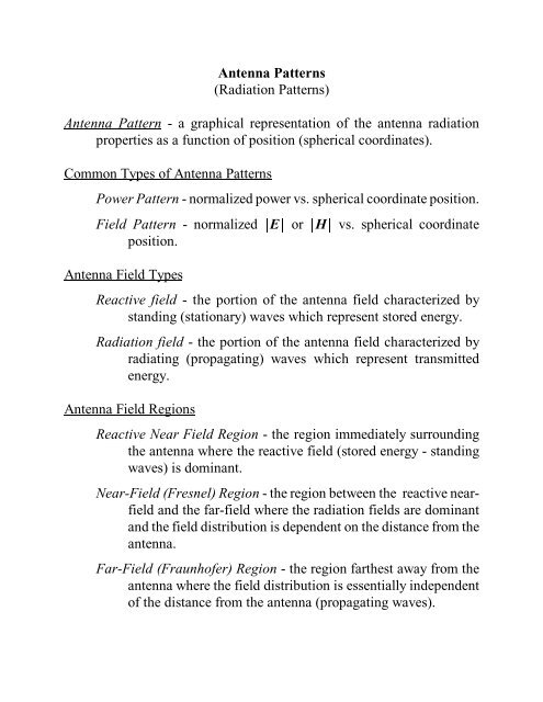
Antenna Pattern DefinitionsIsotropic Pattern - an antenna pattern defined by uniform radiationin all directions, produced by an isotropic radiator (pointsource, a non-physical antenna which is the only nondirectionalantenna).Directional Pattern - a pattern characterized by more efficientradiation in one direction than another (all physically realizableantennas are directional antennas).Omnidirectional Pattern - a pattern which is uniform in a givenplane.Principal Plane Patterns - the E-plane and H-plane patterns of alinearly polarized antenna.E-plane - the plane containing the electric field vectorand the direction of maximum radiation.H-plane - the plane containing the magnetic field vectorand the direction of maximum radiation.Antenna Pattern ParametersRadiation Lobe - a clear peak in the radiation intensity surroundedby regions of weaker radiation intensity.Main Lobe (major lobe, main beam) - radiation lobe in the directionof maximum radiation.Minor Lobe - any radiation lobe other than the main lobe.Side Lobe - a radiation lobe in any direction other than thedirection(s) of intended radiation.Back Lobe - the radiation lobe opposite to the main lobe.

Half-Power Beamwidth (HPBW) - the angular width of the mainbeam at the half-power points.First Null Beamwidth (FNBW) - angular width between the firstnulls on either side of the main beam.Antenna Pattern Parameters(Normalized Power Pattern)

Maxwell’s Equations(Instantaneous and Phasor Forms)Maxwell’s Equations (instantaneous form)(%+' -'%(+'%- - instantaneous vectors [( =( (x,y,z,t), etc.]D t - instantaneous scalarMaxwell’s Equations (phasor form, time-harmonic form)E, H, D, B, J - phasor vectors [E=E(x,y,z), etc.]D - phasor scalarRelation of instantaneous quantities to phasor quantities ...( (x,y,z,t) = Re{E(x,y,z)e jTt }, etc.

Average Power Radiated by an AntennaTo determine the average power radiated by an antenna, we start withthe instantaneous Poynting vector 6 (vector power density) defined by6 (ð+(V/m × A/m = W/m 2 )Assume the antenna is enclosed by some surface S.=s=SdsThe total instantaneous radiated power 3 rad leaving the surface S is foundby integrating the instantaneous Poynting vector over the surface.3 rad ç6@ds = ç((ð+)@ds ds = s dsSS= ds = differential surfaces = unit vector normal to ds=

ReFor time-harmonic fields, the time average instantaneous Poyntingvector (time average vector power density) is found by integrating theinstantaneous Poynting vector over one period (T) and dividing by theperiod.1P avg = ç((ð+) dtT T( = Re{Ee jTt }+ = Re{He jTt }The instantaneous magnetic field may be rewritten as+ = Re{½ [ He jTt + H * e !jTt ]}which gives an instantaneous Poynting vector of(ð+ ½ Re {[E ð H]e j2Tt + [E ð H * ]}~~~~~~~~~~~~~~~ ~~~~~~~time-harmonic(integrates to zero over T )independent of timeand the time-average vector power density becomesP avg = 1[E ð H * ] çdt2TT= ½ Re [E ð H * ]The total time-average power radiated by the antenna (P rad ) is found byintegrating the time-average power density over S.P rad çP avg @ds = ½ Re ç [E ð H * ]@dsSS

Radiation IntensityRadiation Intensity - radiated power per solid angle (radiated powernormalized to a unit sphere).P rad çP avg @dsSIn the far field, the radiation electric and magnetic fields vary as 1/r andthe direction of the vector power density (P avg ) is radially outward. If weassume that the surface S is a sphere of radius r, then the integral for thetotal time-average radiated power becomesIf we defined P avg r 2 = U(2,N) as the radiation intensity, thenwhere d S = sin2d2dN defines the differential solid angle. The units on theradiation intensity are defined as watts per unit solid angle. The averageradiation intensity is found by dividing the radiation intensity by the areaof the unit sphere (4B) which givesThe average radiation intensity for a given antenna represents the radiationintensity of a point source producing the same amount of radiated poweras the antenna.

DirectivityDirectivity (D) - the ratio of the radiation intensity in a given directionfrom the antenna to the radiation intensity averaged over alldirections.The directivity of an isotropic radiator is D(2,N) = 1.The maximum directivity is defined as [D(2,N)] max = D o .The directivity range for any antenna is 0 #D(2,N) #D o .Directivity in dBDirectivity in terms of Beam Solid AngleWe may define the radiation intensity aswhere B o is a constant and F(2,N) is the radiation intensity patternfunction. The directivity then becomesand the radiated power is

Inserting the expression for P rad into the directivity expression yieldsThe maximum directivity iswhere the term S A in the previous equation is defined as the beam solidangle and is defined byBeam Solid Angle - the solid angle through which all of the antennapower would flow if the radiation intensity were [U(2,N)] max for allangles in S A .

Example (Directivity/Beam Solid Angle/Maximum Directivity)Determine the directivity [D(2,N)], the beam solid angle S A and themaximum directivity [D o ] of an antenna defined by F(2,N) =sin 2 2cos 2 2.

In order to find [F(2,N)] max , we must solve

MATLAB m-file for plotting this directivity functionfor i=1:100theta(i)=pi*(i-1)/99;d(i)=7.5*((cos(theta(i)))^2)*((sin(theta(i)))^2);endpolar(theta,d)120902601.51501300.5180 0210330240300270

Directivity/Beam Solid Angle ApproximationsGiven an antenna with one narrow major lobe and negligible radiationin its minor lobes, the beam solid angle may be approximated bywhere 2 1 and 2 2 are the half-power beamwidths (in radians) which areperpendicular to each other. The maximum directivity, in this case, isapproximated byIf the beamwidths are measured in degrees, we haveExample (Approximate Directivity)A horn antenna with low side lobes has half-power beamwidths of29 o in both principal planes (E-plane and H-plane). Determine theapproximate directivity (dB) of the horn antenna.

Numerical Evaluation of DirectivityThe maximum directivity of a given antenna may be written aswhere U(2N) = B o F(2,N). The integrals related to the radiated power inthe denominators of the terms above may not be analytically integrable.In this case, the integrals must be evaluated using numerical techniques.If we assume that the dependence of the radiation intensity on 2 and N isseparable, then we may writeThe radiated power integral then becomes

Note that the assumption of a separable radiation intensity pattern functionresults in the product of two separate integrals for the radiated power. Wemay employ a variety of numerical integration techniques to evaluate theintegrals. The most straightforward of these techniques is the rectangularrule (others include the trapezoidal rule, Gaussian quadrature, etc.) If wefirst consider the 2-dependent integral, the range of 2 is first subdividedinto N equal intervals of lengthThe known function f (2) is then evaluated at the center of eachsubinterval. The center of each subinterval is defined byThe area of each rectangular sub-region is given by

The overall integral is then approximated byUsing the same technique on the N-dependent integral yieldsCombining the 2 and N dependent integration results gives theapproximate radiated power.The approximate radiated power for antennas that are omnidirectional withrespect to N [g(N) = 1] reduces to

The approximate radiated power for antennas that are omnidirectional withrespect to 2 [ f(2) = 1] reduces toFor antennas which have a radiation intensity which is not separable in 2and N, the a two-dimensional numerical integration must be performedwhich yieldsExample (Numerical evaluation of directivity)Determine the directivity of a half-wave dipole given the radiationintensity of

The maximum value of the radiation intensity for a half-wave dipoleoccurs at 2 = B/2 so thatMATLAB m-filesum=0.0;N=input(’Enter the number of segments in the theta direction’)for i=1:Nthetai=(pi/N)*(i-0.5);sum=sum+(cos((pi/2)*cos(thetai)))^2/sin(thetai);endD=(2*N)/(pi*sum)ND o5 1.642810 1.641015 1.640920 1.6409

Antenna EfficiencyWhen an antenna is driven by a voltage source (generator), the totalpower radiated by the antenna will not be the total power available fromthe generator. The loss factors which affect the antenna efficiency can beidentified by considering the common example of a generator connectedto a transmitting antenna via a transmission line as shown below.Z g - source impedanceZ A - antenna impedanceZ o - transmission line characteristic impedanceP in - total power delivered to the antenna terminalsP ohmic - antenna ohmic (I 2 R) losses[conduction loss + dielectric loss]P rad - total power radiated by the antennaThe total power delivered to the antenna terminals is less than thatavailable from the generator given the effects of mismatch at the source/tlineconnection, losses in the t-line, and mismatch at the t-line/antennaconnection. The total power delivered to the antenna terminals must equalthat lost to I 2 R (ohmic) losses plus that radiated by the antenna.

We may define the antenna radiation efficiency (e cd ) aswhich gives a measure of how efficient the antenna is at radiating thepower delivered to its terminals. The antenna radiation efficiency may bewritten as a product of the conduction efficiency (e c ) and the dielectricefficiency (e d ).e c - conduction efficiency (conduction losses only)e d - dielectric efficiency (dielectric losses only)However, these individual efficiency terms are difficult to compute so thatthey are typically determined by experimental measurement. This antennameasurement yields the total antenna radiation efficiency such that theindividual terms cannot be separated.Note that the antenna radiation efficiency does not include themismatch (reflection) losses at the t-line/antenna connection. This lossfactor is not included in the antenna radiation efficiency because it is notinherent to the antenna alone. The reflection loss factor depends on the t-line connected to the antenna. We can define the total antenna efficiency(e o ), which includes the losses due to mismatch ase o - total antenna efficiency (all losses)e r - reflection efficiency (mismatch losses)The reflection efficiency represents the ratio of power delivered to theantenna terminals to the total power incident on the t-line/antenna

connection. The reflection efficiency is easily found from transmissionline theory in terms of the reflection coefficient (').The total antenna efficiency then becomesThe definition of antenna efficiency (specifically, the antenna radiationefficiency) plays an important role in the definition of antenna gain.Antenna GainThe definitions of antenna directivity and antenna gain are essentiallythe same except for the power terms used in the definitions.Directivity [D(2,N)] - ratio of the antenna radiated power density at adistant point to the total antenna radiated power (P rad ) radiatedisotropically.Gain [G(2,N)] - ratio of the antenna radiated power density at a distantpoint to the total antenna input power (P in ) radiated isotropically.Thus, the antenna gain, being dependent on the total power delivered to theantenna input terminals, accounts for the ohmic losses in the antenna whilethe antenna directivity, being dependent on the total radiated power, doesnot include the effect of ohmic losses.

The equations for directivity and gain areThe relationship between the directivity and gain of an antenna may befound using the definition of the radiation efficiency of the antenna.Gain in dB

Antenna ImpedanceThe complex antenna impedance is defined in terms of resistive (real)and reactive (imaginary) components.R A - Antenna resistance[(dissipation ) ohmic losses + radiation]X A - Antenna reactance[(energy storage) antenna near field]We may define the antenna resistance as the sum of two resistances whichseparately represent the ohmic losses and the radiation.R r - Antenna radiation resistance (radiation)R L - Antenna loss resistance (ohmic loss)The typical transmitting system can be defined by a generator,transmission line and transmitting antenna as shown below.The generator is modeled by a complex source voltage V g and a complexsource impedance Z g .

In some cases, the generator may be connected directly to the antenna.Inserting the complete source and antenna impedances yieldsThe complex power associated with any element in the equivalent circuitis given bywhere the * denotes the complex conjugate. We will assume peak valuesfor all voltages and currents in expressing the radiated power, the powerassociated with ohmic losses, and the reactive power in terms of specificcomponents of the antenna impedance. The peak current for the simpleseries circuit shown above is

The power radiated by the antenna (P r ) may be written asThe power dissipated as heat (P L ) may be writtenThe reactive power (imaginary component of the complex power) storedin the antenna near field (P X ) is

From the equivalent circuit for the generator/antenna system, we see thatmaximum power transfer occurs whenThe circuit current in this case isThe power radiated by the antenna isThe power dissipated in heat isThe power available from the generator source is

The power dissipated in the generator resistance isTransmitting antenna system summary (maximum power transfer)Power dissipated inthe generator [P/2]Power available fromthe generator [P]Power dissipated by theantenna [(1!e cd )(P/2)]Power delivered tothe antenna [P/2]Power radiated by theantenna [e cd (P/2)]With an ideal transmitting antenna (e cd = 1) given maximum powertransfer, one-half of the power available from the generator is radiated bythe antenna.

The typical receiving system can be defined by a generator (receivingantenna), transmission line and load (receiver) as shown below.Assuming the receiving antenna is connected directly to the receiverFor the receiving system, maximum power transfer occurs when

The circuit current in this case isThe power captured by the receiving antenna isSome of the power captured by the receiving antenna is re-radiated(scattered). The power scattered by the antenna (P scat ) isThe power dissipated by the receiving antenna in the form of heat isThe power delivered to the receiver is

Receiving antenna system summary (maximum power transfer)Power delivered tothe receiver [P/2]Power captured bythe antenna [P]Power dissipated by theantenna [(1!e cd )(P/2)]Power delivered tothe antenna [P/2]Power scattered by theantenna [e cd (P/2)]With an ideal receiving antenna (e cd = 1) given maximum power transfer,one-half of the power captured by the antenna is re-radiated (scattered) bythe antenna.

Antenna Radiation EfficiencyThe radiation efficiency (e cd ) of a given antenna has previously beendefined in terms of the total power radiated by the antenna (P rad ) and thetotal power dissipated by the antenna in the form of ohmic losses (P ohmic ).The total radiated power and the totalohmic losses were determined for thegeneral case of a transmitting antennausing the equivalent circuit. The totalradiated power is that “dissipated” inthe antenna radiation resistance (R r ).The total ohmic losses for the antenna are those dissipated in the antennaloss resistance (R L ).Inserting the equivalent circuit results for P rad and P ohmic into the equationfor the antenna radiation efficiency yieldsThus, the antenna radiation efficiency may be found directly from theantenna equivalent circuit parameters.

Antenna Loss ResistanceThe antenna loss resistance (conductor and dielectric losses) for manyantennas is typically difficult to calculate. In these cases, the lossresistance is normally measured experimentally. However, the lossresistance of wire antennas can be calculated easily and accurately.Assuming a conductor of length l and cross-sectional area A which carriesa uniform current density, the DC resistance iswhere F is the conductivity of the conductor. At high frequencies, thecurrent tends to crowd toward the outer surface of the conductor (skineffect). The HF resistance can be defined in terms of the skin depth *.where : is the permeability of the material and f is the frequency in Hz.The skin depth for copper (F = 5.8×10 7 ®/m, : = : o = 4B×10 !7 H/m) maybe written as

If we define the perimeter distance of the conductor as d p , then the HFresistance of the conductor can be written aswhere R s is defined as the surface resistance of the material.For the R HF equation to be accurate, the skin depth should be a smallfraction of the conductor maximum cross-sectional dimension. In the caseof a cylindrical conductor (d p . 2Ba), the HF resistance isf * R0 4 R DC = 0.818 mS1 kHz 2.09 mm ~10 kHz 0.661 mm R HF = 1.60 mS100 kHz 0.209 mm R HF = 5.07 mS1 MHz 0.0661mmR HF = 16.0 mSResistance of 1 m of #10 AWG (a = 2.59 mm) copper wire.

The high frequency resistance formula assumes that the current through theconductor is sinusoidal in time and independent of position along theconductor [I z (z,t) = I o cos(Tt)]. On most antennas, the current is notnecessarily independent of position. However, given the actual currentdistribution on the antenna, an equivalent R L can be calculated.Example (Problem 2.44) [Loss resistance calculation]A dipole antenna consists of a circular wire of length l. Assuming thecurrent distribution on the wire is cosinusoidal, i.e.,Equivalent circuit equation(uniform current, I o - peak)Integration of incrementalpower along the antenna

Thus, the loss resistance of a dipole antenna of length l is one-half that ofa the same conductor carrying a uniform current.

Lossless Transmission Line FundamentalsTransmission line equations (voltage and current)~~~~~~~ ~~~~~~~+z directed !z directedwaves waves

Transmitting/Receiving Systems with Transmission LinesUsing transmission line theory, the impedance seen looking intothe input terminals of the transmission line (Z in ) isThe resulting equivalent circuit is shown below.The current and voltage at the transmission line input terminals are

The power available from the generator isThe power delivered to the transmission line input terminals isThe power associated with the generator impedance isGiven the current and the voltage at the input to the transmission line, thevalues at any point on the line can be found using the transmission lineequations.The unknown coefficient V o+ may be determined from either V(0) or I(0)which were found in the input equivalent circuit. Using V(0) gives

whereGiven the coefficient V o+ , the current and voltage at the load, from thetransmission line equations areThe power delivered to the load is thenThe complexity of the previous equations leads to solutions which aretypically determined by computer or Smith chart.

MATLAB m-file (generator/t-line/load)Vg=input(’Enter the complex generator voltage ’);Zg=input(’Enter the complex generator impedance ’);Zo=input(’Enter the lossless t-line characteristic impedance ’);l=input(’Enter the lossless t-line length in wavelengths ’);Zl=input(’Enter the complex load impedance ’);j=0+1j;betal=2*pi*l;Zin=Zo*(Zl+j*Zo*tan(betal))/(Zo+j*Zl*tan(betal));gammal=(Zl-Zo)/(Zl+Zo);gamma0=gammal*exp(-j*2*betal);Ig=Vg/(Zg+Zin);Pg=0.5*Vg*conj(Ig);V0=Ig*Zin;P0=0.5*V0*conj(Ig);Vcoeff=V0/(1+gamma0);Vl=Vcoeff*exp(-j*betal)*(1+gammal);Il=Vcoeff*exp(-j*betal)*(1-gammal)/Zo;Pl=0.5*Vl*conj(Il);s=(1+abs(gammal))/(1-abs(gammal));format compactGenerator_voltage=VgGenerator_current=IgGenerator_power=PgGenerator_impedance_voltage=Vg-V0Generator_impedance_current=IgGenerator_impedance_power=Pg-P0T_line_input_voltage=V0T_line_input_current=IgT_line_input_power=P0T_line_input_impedance=ZinT_line_input_reflection_coeff=gamma0T_line_standing_wave_ratio=sLoad_voltage=VlLoad_current=IlLoad_power=PlLoad_reflection_coeff=gammalGiven V g = (10+j0) V, Z g = (100+j0) S and l = 5.1258, the following results are found.Z o Z L Z in *'(0)*=*'(l)* P g s P(l)100 75 96+j28 0.1429 0.25 1.3333 0.1224100 100 100 0 0.25 1 0.125100 125 98!j22 0.1111 0.25 1.25 0.123575 100 72!j21 0.1429 0.2864 1.3333 0.1199100 100 100 0 0.25 1 0.125125 100 122+j27 0.1111 0.2219 1.25 0.1219

Antenna PolarizationThe polarization of an plane wave is defined by the figure traced bythe instantaneous electric field at a fixed observation point. The followingare the most commonly encountered polarizations assuming the wave isapproaching.

The polarization of the antenna in a given direction is defined as thepolarization of the wave radiated in that direction by the antenna. Notethat any of the previous polarization figures may be rotated by somearbitrary angle.Polarization loss factorIncident wave polarizationAntenna polarizationPolarization loss factor (PLF)PLF in dB

General Polarization EllipseThe vector electric field associated with a +z-directed plane wave canbe written in general phasor form aswhere E x and E y are complex phasors which may be defined in terms ofmagnitude and phase.

The instantaneous components of the electric field are found bymultiplying the phasor components by e jT t and taking the real part.( x (z,t)( y (z,t)The relative positions of the instantaneous electric field components on thegeneral polarization ellipse defines the polarization of the plane wave.Linear PolarizationIf we define the phase shift between the two electric fieldcomponents aswe find that a phase shift ofdefines a linearly polarized wave.( x (z,t)( y (z,t)Examples of linear polarization:If E yo = 0 Y Linear polarization in the x-direction (J = 0)If E xo = 0 Y Linear polarization in the y-direction (J = 90 o )If E xo = E yo and n is even Y Linear polarization (J = 45 o )If E xo = E yo and n is odd Y Linear polarization (J = 135 o )

Circular PolarizationIf E xo = E yo andthen( y (z,t)( x (z,t)This is left-hand circular polarization.If E xo = E yo andthen( x (z,t)( y (z,t)This is right-hand circular polarization.Elliptical PolarizationElliptical polarization follows definitions as circular polarizationexcept that E xo ú E yo .E xo ú E yo , )N = (2n+½)B Y left-hand elliptical polarizationE xo ú E yo , )N = !(2n+½)B Y right-hand elliptical polarization

Antenna Effective Aperture (Area)Antenna Equivalent AreasGiven a receiving antenna oriented for maximum response,polarization matched to the incident wave, and impedance matched to itsload, the resulting power delivered to the receiver (P rec ) may be defined interms of the antenna effective aperture (A e ) aswhere S is the power density of the incident wave (magnitude of thePoynting vector) defined byAccording to the equivalent circuit under matched conditions,We may solve for the antenna effective aperture which gives

Antenna Scattering AreaThe total power scattered by the receiving antenna is defined as theproduct of the incident power density and the antenna scattering area (A s ).From the equivalent circuit, the total scattered power iswhich givesAntenna Loss AreaThe total power dissipated as heat by the receiving antenna is definedas the product of the incident power density and the antenna loss area(A L ).From the equivalent circuit, the total dissipated power iswhich gives

Antenna Capture AreaThe total power captured by the receiving antenna (power deliveredto the load + power scattered by the antenna + power dissipated in the formof heat) is defined as the product of the incident power density and theantenna capture area (A c ).The total power captured by the antenna iswhich givesNote that A c = A e + A s + A L .

Maximum Directivity and Effective ApertureAssume the transmitting and receiving antennas are lossless andoriented for maximum response.A et , D ot - transmit antenna effective aperture and maximum directivityA er , D or - receive antenna effective aperture and maximum directivityIf we assume that the total power transmitted by the transmit antenna is P t ,the power density at the receive antenna (W r ) isThe total power received by the receive antenna (P r ) iswhich givesIf we interchange the transmit and receive antennas, the previousequation still holds true by interchanging the respective transmit andreceive quantities (assuming a linear, isotropic medium), which gives

These two equations yieldorIf the transmit antenna is an isotropic radiator, we will later show thatwhich givesTherefore, the equivalent aperture of a lossless antenna may be defined interms of the maximum directivity asThe overall antenna efficiency (e o ) may be included to account for theohmic losses and mismatch losses in an antenna with losses.The effect of polarization loss can also be included to yield

Friis Transmission EquationThe Friis transmission equation defines the relationship betweentransmitted power and received power in an arbitrary transmit/receiveantenna system. Given arbitrarily oriented transmitting and receivingantennas, the power density at the receiving antenna (W r ) iswhere P t is the input power at the terminals of the transmit antenna andwhere the transmit antenna gain and directivity for the system performanceare related by the overall efficiencywhere e cdt is the radiation efficiency of the transmit antenna and ' t is thereflection coefficient at the transmit antenna terminals. Notice that thisdefinition of the transmit antenna gain includes the mismatch losses for thetransmit system in addition to the conduction and dielectric losses. Amanufacturer’s specification for the antenna gain will not include themismatch losses.The total received power delivered to the terminals of the receivingantenna (P r ) iswhere the effective aperture of the receiving antenna (A er ) must take into

account the orientation of the antenna. We may extend our previousdefinition of the antenna effective aperture (obtained using the maximumdirectivity) to a general effective aperture for any antenna orientation.The total received power is thensuch that the ratio of received power to transmitted power isIncluding the polarization losses yieldsFor antennas aligned for maximum response, reflection-matched andpolarization matched, the Friis transmission equation reduces to

Radar Range Equation and Radar Cross SectionThe Friis transmission formula can be used to determine the radarrange equation. In order to determine the maximum range at which a giventarget can be detected by radar, the type of radar system (monostatic orbistatic) and the scattering properties of the target (radar cross section)must be known.Monostatic radar system - transmit and receive antennas at thesame location.Bistatic radar system- transmit and receive antennas at separatelocations.

Radar cross section (RCS) - a measure of the ability of a target to reflect(scatter) electromagnetic energy (units = m 2 ). The area which interceptsthat amount of total power which, when scattered isotropically,produces the same power density at the receiver as the actual target.If we defineF = radar cross section (m 2 )W i = incident power density at the target (W/m 2 )P c = equivalent power captured by the target (W)W s = scattered power density at the receiver (W/m 2 )According to the definition of the target RCS, the relationship between theincident power density at the target and the scattered power density at thereceive antenna isThe limit is usually included since we must be in the far-field of the targetfor the radar cross section to yield an accurate result.

The radar cross section may be written aswhere (E i , H i ) are the incident electric and magnetic fields at the target and(E s , H s ) are the scattered electric and magnetic fields at the receiver. Theincident power density at the target generated by the transmitting antenna(P t , G t , D t , e ot , ' t , a t ) is given byThe total power captured by the target (P c ) isThe power captured by the target is scattered isotropically so that thescattered power density at the receiver isThe power delivered to the receiving antenna load is

Showing the conduction losses, mismatch losses and polarization lossesexplicitly, the ratio of the received power to transmitted power becomeswherea w - polarization unit vector for the scattered wavesa r - polarization unit vector for the receive antennaGiven matched antennas aligned for maximum response and polarizationmatched, the general radar range equation reduces to

ExampleProblem 2.65 A radar antenna, used for both transmitting andreceiving, has a gain of 150 at its operating frequency of 5 GHz. Ittransmits 100 kW, and is aligned for maximum directional radiation andreception to a target 1 km away having a cross section of 3 m 2 . Thereceived signal matches the polarization of the transmitted signal. Find thereceived power.